What do we perceive in a glance of a real-world scene?
←
→
Page content transcription
If your browser does not render page correctly, please read the page content below
Journal of Vision (2007) 7(1):10, 1–29                    http://journalofvision.org/7/1/10/                                              1

What do we perceive in a glance of a real-world scene?
                                                           Computer Science Department, Princeton University,
Li Fei-Fei                                                                               Princeton, NJ, USA

                                           Division of Biological Sciences, California Institute of Technology,
Asha Iyer                                                                                Pasadena, CA, USA

                                           Division of Biological Sciences, California Institute of Technology,
Christof Koch                                                                            Pasadena, CA, USA

                                         Electrical Engineering Department, California Institute of Technology,
Pietro Perona                                                                            Pasadena, CA, USA

What do we see when we glance at a natural scene and how does it change as the glance becomes longer? We asked
naive subjects to report in a free-form format what they saw when looking at briefly presented real-life photographs. Our
subjects received no specific information as to the content of each stimulus. Thus, our paradigm differs from previous
studies where subjects were cued before a picture was presented and/or were probed with multiple-choice questions. In the
first stage, 90 novel grayscale photographs were foveally shown to a group of 22 native-English-speaking subjects. The
presentation time was chosen at random from a set of seven possible times (from 27 to 500 ms). A perceptual mask
followed each photograph immediately. After each presentation, subjects reported what they had just seen as completely
and truthfully as possible. In the second stage, another group of naive individuals was instructed to score each of the
descriptions produced by the subjects in the first stage. Individual scores were assigned to more than a hundred different
attributes. We show that within a single glance, much object- and scene-level information is perceived by human subjects. The
richness of our perception, though, seems asymmetrical. Subjects tend to have a propensity toward perceiving natural scenes
as being outdoor rather than indoor. The reporting of sensory- or feature-level information of a scene (such as shading and
shape) consistently precedes the reporting of the semantic-level information. But once subjects recognize more semantic-level
components of a scene, there is little evidence suggesting any bias toward either scene-level or object-level recognition.
Keywords: perception, natural scene, real-world scene, indoor, outdoor, sensory-level perception, segmentation,
object recognition, subordinate, entry level, superordinate, object categorization, scene categorization, event recognition,
free recall
Citation: Fei-Fei, L., Iyer, A., Koch, C., & Perona, P. (2007). What do we perceive in a glance of a real-world scene? Journal
of Vision, 7(1):10, 1–29, http://journalofvision.org/7/1/10/, doi:1 0. 116 7 /7 .1 .1 0 .

 Introduction                                                                 although the semantic understanding of a scene is quickly
                                                                              extracted, it requires a few hundred milliseconds to be
                                                                              consolidated into memory (Potter, 1976). Later studies
  It is known that humans can understand a real-world scene                   documented limits to our perception of a scene. Rensink,
quickly and accurately, saccading many times per second                       O’Regan, and Clark (1997) showed that changes to
while scanning a complex scene. Each of these glances                         retinotopically large portions of the scene will sometimes
carries considerable information. Filmmakers have long                        go unobserved. It is likely that this occurs if the regions
exploited this ability through a technique called Bflash cut.[                are not linked to the scene’s overall Bmeaning.[
In a commercial motion picture called The Pawnbroker                             Other hallmark investigations attempted to elucidate the
(Lumet, 1965), S. Lumet inserted an unusually brief scene                     information involved in this Boverall meaning[; their
that represented a distant memory. Lumet found that a                         conclusions regarding scene perception paralleled con-
presentation lasting a third of a second, although unexpected                 cepts in auditory studies of sentence and word compre-
and unrelated to the flow of the main narrative, was sufficient               hension. Biederman et al. found that recognition of objects
for the audience to capture the meaning of the interposed                     is impaired when those objects are embedded in a randomly
scene (Biederman, Teitelbaum, & Mezzanotte, 1983).                            jumbled rather than a coherent scene (Biederman, 1972).
  Pioneering studies extended these anecdotal findings.                       They identified several physical (support, interposition)
Potter (1976) and Potter, Staub, Rado, and O’Connor                           and semantic (probability, position, size) constraints that
(2002) utilized rapid serial visual presentations of images                   objects must satisfy within a scene, similar to the syntactic
and revealed that subjects could perceive scene content in                    and grammatical rules of language (Biederman, 1982).
less than 200 ms. Furthermore, Potter demonstrated that                       They investigated how object recognition was modulated
doi: 1 0. 11 67 / 7 . 1 . 10                 Received December 30, 2005; published January 31, 2007                   ISSN 1534-7362 * ARVO
Journal of Vision (2007) 7(1):10, 1–29 Fei-Fei, Iyer, Koch, & Perona 2
by violating these constraints. They concluded that the 3. One parameter to vary in examining scene perception
schema of a sceneVor the overall internal representation is the length of PTs. We are curious to see whether
of a scene that includes objects and object relationsVis different percepts arise in a given temporal order.
perceived within a single fixation (Biederman, 1982),
regardless of expectation and familiarity (Biederman et al., In the Method section, we introduce in detail our
1983). Boyce, Pollatsek, and Rayner (1989) also demon- experimental paradigm. We first show the images used
strated that objects are more difficult to identify when in our experiments (Stimuli section). The Experimental
located against an inconsistent background given a Stage I section describes how we collected image
briefly flashed scene (150 ms), further suggesting that descriptions. The Experimental Stage II section then
both recognition of objects and global contextual under- explicates how these descriptions are evaluated. Five
standing are quickly and deftly accomplished. different observations are presented in the Results and
These studies show that some comprehension of a scene Observations section. We summarize our findings and
is rapidly attained. However, in all previous studies of general discussions in the Conclusion section.
scene perception, the experimenters have a set of
predetermined hypotheses to test. Their experiments are
hence constructed to illuminate certain parameters rele-
vant to their claims and questions. As a number of Method
questions are left unexplored by this approach, we propose
to examine unbiased real-world scene perception as a
function of display time. We have designed an experiment Our subjects were asked to freely recall what they
in which subjects view one of nearly a hundred novel perceive in briefly displayed images of real-world scenes.
natural scenes for a brief interval without any priming and We explored the evolution of our subjects’ reports as a
pre- or poststimulus cuing, as to its content. We ask them function of the length of PTs. Our data were collected in
to type freely what they have seen in as much detail as Stage I and analyzed in Stage II.
possible. We vary the presentation time (PT) of the image In Stage I, subjects viewed briefly a picture of a scene
between 27 ms and 500 ms. Through unbiased responses, on a computer monitor and were then asked to type what
we hope to uncover new aspects of scene perception that they had seen, using a free-recall method to collect
were previously not considered. The following issues arose responses. The Experimental Stage I section explains the
when we examined the free-recall responses we collected. details of this stage of the experiment.
In Stage II, we asked an independent group of subjects
1. There has been no commonly accepted definition of to evaluate and classify the free-recall responses collected
the content of Bgist.[ Mandler and Parker (1976) have in Stage I. The Experimental Stage II section is a detailed
suggested that three types of information are remem- account of this evaluation process.
bered from a picture: (i) an inventory of objects, (ii)
descriptive information of the physical appearance
and other details of the objects, and (iii) spatial rela- Stimuli
tions between the objects. In addition to this object
information, propositional relationships between ob- In most previous studies of scene perception or
jects, spatial layout of the scene, and a general im- object recognition, line drawings were used as stimuli
pression of the low-level features that fill the scene (Biederman, 1982; Hollingworth & Henderson, 1999).
(e.g., texture) are speculatively incorporated into the Recently, several studies have used a large commercial
scene gist (Wolfe, 1998a). Finally, Biederman (1982) database of photographs to study the perception of scenes
has proposed that global semantic meaning or con- and categories (Li, VanRullen, Koch, & Perona, 2002;
text also contributes to the initial surmisal of a scene. Thorpe, Fize, & Marlot, 1996; Torralba & Oliva, 2003).
Positing the Bcontents[ of a glance as an operational This data set, unfortunately, is a collection of profes-
definition of scene gist, we would like to ascertain sionally photographed scenes, mostly shot with the goal
the visual and semantic information comprising scene of capturing a single type of objects or specific themes of
gist, as revealed by our subjects’ responses. scenes. We are, however, interested in studying images of
2. Rosch (1978) suggested that one distinguishes everyday scenes, as commonly seen by most people in a
between Bbasic-level,[ Bsuperordinate-level,[ and naturalistic setting.1 Therefore, we assembled a collection
Bsubordinate-level[ object categories. Similarly, of images trying to minimize this sampling bias.
Tversky and Hemenway (1983) proposed the same Figures 1 and 2 show our data set of 44 indoor images
taxonomy for scene categories. These authors motivate and 46 outdoor images collected from the Internet in the
their theory with arguments of maximizing the visual following way. We asked a group of 10 naive subjects to
and linguistic information conveyed during naming. randomly call out five names of scenes that first came to
Does human perception of natural complex scenes their mind. Some of the names overlapped. After pruning,
reveal a similar hierarchy of objects and scenes? we retained about 25 to 30 different words or wordJournal of Vision (2007) 7(1):10, 1–29 Fei-Fei, Iyer, Koch, & Perona 3 Figure 1. Forty-six images of outdoor scenes in our data set of 90 grayscale images.
Journal of Vision (2007) 7(1):10, 1–29                 Fei-Fei, Iyer, Koch, & Perona   4

Figure 2. Forty-four images of indoor scenes in our data set of 90 grayscale images.
Journal of Vision (2007) 7(1):10, 1–29                  Fei-Fei, Iyer, Koch, & Perona                                                  5

phrases that corresponded to different environments.2 We                 Stage I. One author (A.I.) was among the subjects. All
typed each of these words or word phrases in the Google                  subjects (including A.I.) were naive about the purpose of
image search engine. From the first few page(s) of search                the experiments until all data were collected.
results, we randomly selected 3–6 images that depicted
the keyword. The Google image search engine largely
returned images found on people’s personal websites,                     Apparatus
most often taken with a snapshot camera. Although                          Subjects were seated in a dark room especially designed
everyone has a bias when taking a picture, we believe                    for psychophysics experiments. The seat was approxi-
that the large number of images from different unknown                   mately 100 cm from a computer screen, connected to a
sources would help average out these biases.                             Macintosh (OS9) computer. The refresh rate of the
   A number of authors have suggested that color                         monitor was 75 Hz. All experimental software was
information is not critical for the rapid categorization of              programmed using the Psychophysics Toolbox (Brainard,
scenes (Fabre-Thorpe, Delorme, Marlot, & Thorpe, 2001;                   1997; Pelli, 1997) and MATLAB.
Fei-Fei et al., 2005). While color could be diagnostic in a
later stage of recognition (Oliva & Schyns, 2000), and
                                                                         Procedure
uncommon colors might even hinder rapid scene catego-
rization (Goffaux, Jacques, Mauraux, Oliva, Schynsand, &                   Figure 3 illustrates a single trial of Stage I. An image
Rossion, 2005), we are mostly concerned with the initial                 from our data set was presented for one of seven different
evolution of scene perception. Thus, we decided to use only              possible PTs: 27, 40, 53, 67, 80, 107, and 500 ms. For
grayscale versions of our images for our experiments. It will            each trial, the particular PT was randomly selected with
be, however, interesting to compare our results with a                   equal probability from these choices. The image was then
future study using colored images.                                       masked by one of eight natural image perceptual masks,
                                                                         constructed by superposing white noise band-passed at
                                                                         different spatial frequencies (Li et al., 2002; VanRullen, &
Experimental Stage I: Free recall                                        Koch, 2003). The subject was then shown a screen with
Subjects                                                                 the words:
  Twenty-two highly motivated California Institute of                        Please describe in detail what you see in the picture.
Technology students (from 18 to 35 years old) who were                       Two sample responses are: 1. City scene. I see a big
proficient in English served as subjects in Experiment                       building on the right, and some people walking by

Figure 3. A single trial in Stage I: A fixation cross appeared for about 250 ms. An image from our data set was then presented at the
center, subtending 6-  8- in visual angle. After a variable PT, the image was masked by one of eight natural image perceptual masks (for
details of the mask, see Li et al., 2002). The time between the onset of the image and the onset of the mask is called the PT. The mask
was presented for 500 ms. Afterward, subjects were prompted to a screen in which they were asked to type in what they had seen of the
image. Subjects were given an unlimited amount of time to write down their responses. When they were ready to continue, they could
initiate the next trial by pressing the space bar.
Journal of Vision (2007) 7(1):10, 1–29 Fei-Fei, Iyer, Koch, & Perona 6
shops. There are also trees. Most of the trees are on As scorers needed to analyze and interpret unstructured
the left of the picture, against some background written responses, they were required to be native English
buildings. 2. Possibly outdoor. I really cannot tell speakers. All scorers were naive about the purpose of the
much. Probably some animals, maybe mammalsI experiments until all response evaluation was finished.
Subjects were given an unlimited amount of time to
write down their responses. Apparatus
Each subject was shown all 90 images in the database, The scorers’ task was to evaluate and classify the image
broken into five 22-trial sessions. The images were descriptions obtained in the previous stage. For this
presented in random order. At the beginning of each purpose, they used Response Analysis software that we
session, 4 images outside of the database were used to designed and implemented for this purpose (Figure 5).
familiarize the subject with the responses and PTs. Free- Subjects were seated in a lighted office room. The seat
recall responses for these 20 (4 5) images were was approximately 100 cm from a computer screen,
excluded from all data analysis. Order of image presenta- connected to a Macintosh (OS9) computer. The refresh
tion, as well as the choice of PT for each image, was rate of the monitor was 75 Hz. All Response Analysis user
randomized among all subjects. Each subject thus con- interface software was programmed using MATLAB and
tributed one description for each image at one of the PTs. the GUI toolbox.
Overall, our 22 subjects provided 1,980 descriptions; that
is, we obtained between 3 and 4 descriptions for each
image and each PT. Procedure
Our aim was to evaluate free-recall responses in a
consistent and uniform manner for all subjects. To do this,
Experimental Stage II: Description evaluation we assessed the content of all responses with respect to a
standardized list of attributes.
Subjects The list of attributes was constructed by the experi-
Five paid volunteer undergraduate students from menters, who examined the entire set of free-recall
different schools in the Los Angeles area (from 18 to responses/descriptions to extract a comprehensive inven-
35 years old) served as scorers in Experiment Stage II. tory of terms referred to in these descriptions. Most
Figure 4. Attribute tree. The list of attributes was constructed by examining the entire set of free-recall responses/descriptions to extract a
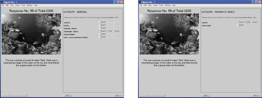
comprehensive inventory of terms referred to in these descriptions.Journal of Vision (2007) 7(1):10, 1–29 Fei-Fei, Iyer, Koch, & Perona 7 Figure 5. Experiment Stage II: Evaluating the free-recall responses. This figure is best viewed with magnification. attributes described fell into one of six categories: Analysis interface tool (Figure 5). For each response, inanimate objects, animate objects, outdoor scenes, indoor the scorer proceeded as follows: the first screen contained scenes, visual/perceptual features (i.e., shapes, lines), or the text of one of the responses, the image described in the event related (this category comprised a more cognitive response, and a box with labels for the most general understanding of the picture, in which human behavior attributes: indoor, outdoor, animate object, inanimate related to the scene was inferred, i.e., social interaction, object, event related, and shape related. Next to each sports/games, performances, concert; see Figure 4 for the attribute, a button allowed the scorer to indicate whether entire list of attributes). It goes without saying that this the attribute had been described in the written response. If attribute tree is not a complete reflection of everything an attribute was checked as Bdescribed,[ the scorer was reported by subjects. We chose to focus on descriptions of additionally required to indicate whether the description sensory information (e.g., shape, shading), objects and of the attribute was either an Baccurate[ or Binaccurate[ scenes, rather than on more cognitive functionalities such depiction of the corresponding image. This completed the as emotions. In addition, explicit verbal reports are likely first screen. For any attribute checked, a successive screen to indicate a lower bound of perceived information limited was displayed, which, again, comprised the text of the by both short-term memory as well as a natural tendency response and the image, but instead of the general of reporting more abstractly than what has been seen. attributes, the next level of more detailed attributes was The attribute list consisted of 105 terms. We organized used; for example, if inanimate object had been checked these attributes into a hierarchical tree structure, where the in the first screen, a following screen would have highest level represented the most general level of descrip- contained the labels manmade and natural (Figure 4), tion (e.g., inanimate object); the intermediate stages for which the user would again be prompted to indicate exhibited a greater degree of specificity (e.g., manmade whether these attributes were described in the response, inanimate object, building); and the lowest level corre- and if so, whether they were accurately or inaccurately sponded to the most detailed level of description (e.g., described. If the user had then checked natural, a Capitol building). This taxonomy schema stems from following screen would have contained the text of the conventional notions of object and scene categorization, as response, the image, and the next level of attributes: body originally developed by Rosch (1978) and Tversky and of water, plant, specific plant, mountain/hill, and distinc- Hemenway (1983), predicated on the superordinate level, tive texture. The entire branch was thus traversed. the entry (or basic) level, and the subordinate level. The If, on the first screen, the scorer had also checked indoor, findings of these authors formed the basis of our hierarch- then subsequent screens would have also displayed the text ical classification for the animate object, inanimate object, of the response, the image, and the next level of attributes: indoor, and outdoor branches of the tree. The last two store, household room, kitchen, office/classroom, technical branches Vsensory related and event related Vhave environment, dining/restaurant, station/plaza, library, and received less investigation and, thus, were classified performance venue. In this manner, the relevant portions of parsimoniously with only two levels: more general (e.g., the tree were traversed, one branch at a time. This process sensory related) and more detailed (e.g., lines, shapes). was repeated for each response. Each of the five scorers read every response (22 subjects As explicated earlier, three to four responses were who each responded to the same 90 images, for a total of provided for a given image at a given PT. For a given 1,980 responses) and assayed them for mention or attribute, each scorer judged whether each of these three description of each attribute as well as correctness. The to four responses accurately described the attribute in the scorer was guided through this task with the Response respective image. The percentage of responses rated as
Journal of Vision (2007) 7(1):10, 1–29                      Fei-Fei, Iyer, Koch, & Perona                                                   8

                                                                                Because this is the primary analysis employed, we
                                                                             will focus on the evaluation of one attribute, building, to
                                                                             better illustrate the parameters just discussed (depicted in
                                                                             Figure 6).
                                                                                On the x-axis are the seven PTs for which images were
                                                                             displayed. The y-axis reflects normalized accuracy evalu-
                                                                             ation score. For the PT of 80 ms, for example, each scorer
                                                                             sees roughly three responses for each image. For each
                                                                             response, the scorer determines whether the attribute
                                                                             building was accurately reported with respect to the
                                                                             corresponding image (the other 104 attributes were also
                                                                             checked, but we will not follow those for the purposes of
                                                                             this example.) Suppose that the scorer indicates that
                                                                             building was described accurately in only one response.
                                                                             The initial evaluation score for the attribute building for
                                                                             this image at PT 80 ms is therefore 1/3 or 0.33. Suppose
Figure 6. A sample score plot for the building attribute.
                                                                             also that the maximum accuracy score achieved in
                                                                             describing this image occurred at PT 500 ms, where two
accurate measured the Bdegree[ to which the attribute was                    thirds of the responses accurately reported a building. This
perceived in this image. This initial score thus reflected a                 maximum score of 0.67 would be used to normalize all
particular image, PT, and scorer. The scores were then                       scores so that the evaluation score PT 80 ms is now 0.5
normalized: The seven scores for a given image (one for                      and the score at 500 ms is 1.0. This normalization allows
each PT) were divided by the highest score achieved for                      each image to be its own baseline; therefore, differences in
that image (across all PTs). All evaluation scores were                      the quality of the image (i.e., simple vs. cluttered, see
therefore between 0 and 1. Due to this Bwithin-image[                        Figure 7) will not affect scores. Finally, all normalized
normalization, inherent differences in Bdifficulty[ of                       building scores at PT 80 msVone for each imageVare
perceiving or understanding scenes between different                         averaged to obtain the final evaluation score at this PT for
images were eliminated.                                                      this particular scorer.
   These scores were then utilized in three general kinds of                    This process of normalization per image and then
analyses, depending on the issues we were interested in                      averaging over all images is done for each PT. Again,
exploring. Most questions we asked fall into the realm of                    the resulting values are per scorer. Thus, in Figure 6, the
characterizing the content of subject’s perception. Hence,                   yellow, blue, green, cyan, and magenta lines each
in the first type of analysis, the evaluation scores were                    represent the normalized evaluation scores (averaged over
further averaged over images so that the averaged evalua-                    images) for one scorer. These curves are then averaged
tion score represented the degree to which the attribute was                 over all the scorers. The resulting means are plotted in the
perceived at a given PT across the entire image set.                         red line in Figure 6, with error bars representing standard
Finally, the scores were averaged over all five scorers.                     error of the mean.

Figure 7. Subject description samples. In the first row, the scene is relatively easy. Subjects are nearly as good at perceiving the details of
the scene at PT 107 ms compared to PT 500 ms. In the second row, the scene is more cluttered and complex.
Journal of Vision (2007) 7(1):10, 1–29 Fei-Fei, Iyer, Koch, & Perona 9 In addition, there is a black line resting at the bottom of scene context versus their perception of objects within the the plot. It consists of scores given by our scorers when scene and whether separate and independent mechanisms the responses/descriptions are randomly matched to the operated for these two kinds of perception (Observation IV images. This serves as a control in the response evaluation employs this kind of correlation analysis.) To do this, process. As this evaluation process is subjective, scorer we created a scatter plot for each PT (e.g., Figure 17a). bias in judging accuracy of responses could be a potential Each dot on the scatter plot represents one image. One of confound; that is, a scorer might be inclined to generally the attributes, for example, scene, is taken as a bench- interpret vague or nebulous responses as Bprobably mark. The red dots represent the images with the top 20% correct,[ giving Bthe benefit of the doubt[ even for in- of evaluation scores for scene, at the baseline condition accurate descriptions. To probe for this bias, we presented (PT 500 ms). The green dots are the images with the each scorer with 220 responses that were paired with an lowest 20% of evaluation scores for scene at the baseline incorrect image (e.g., not the image the subject was view- condition. The black dots represent the remaining images. ing when making the response). The scorer had to indicate These images’ evaluation scores for the scene attribute are whether the response accurately described the image plotted according to the x-axis; their object attribute with which it was presented, the same task as for the real scores are plotted against the y-axis. On each scatter plot, response–image pairings. Because these are incorrect pair- we also show the correlation coefficient (between scene ings, responses associated with longer PTs will not con- and object scores) computed across all images. This can tain a more accurate description of any attribute (in this be done for any pair of attributes. case, building) of the image with which it is presented to We now detail the observations that followed from the scorer. Therefore, assuming no scorer bias, the line these various analyses. should remain low and flat, as observed in Figure 6. The control curves from all scorers were averaged. Weibull cumulative density functions are also fitted to the evaluation scores for each attribute to further confirm Results and Observations trends indicated by the scores across PTs (see Appendix C for details). The second kind of analysis is performed to contrast Observation I: The ‘‘content’’ of a single subjects’ perception with reality, that is, to determine if fixation systematic discrepancies exist between the stimulus and the perception of the stimulus. For this objective, each image is How much of a scene can be initially perceived within examined separately, and the normalized evaluation scores the first glance? for that image are compared with the Bground-truth[ Bar and Ullman (1996) and Friedman (1979) proposed classification of that image (Observation II results from this that early scene recognition involves the identification of kind of analysis). As an example, we take the attributes at least one Bobligatory[ object. In this Bpriming model,[ indoor and outdoor. The process of arriving at a normal- the obligatory object serves as a contextual pivotal point ized evaluation score for each image at a given PT has for the recognition of other parts of the scene (Henderson already been explicated; these scores are then averaged & Hollingworth, 1999). There is also evidence that objects over all scorers, reflecting essentially the percentage of could be independently recognized without facilitation by responses indicating that the attribute was perceived in this global scene context (Henderson & Hollingworth, 1999). image. Ground-truth is determined in the following way: Biederman’s findings however implied that some kind of for each image, we take all responses of all subjects at PT global context of the scene is registered in the early stages 500 ms. If most of the subjects accurately described the of scene and object recognition (Biederman, 1972). Given image as Boutdoor,[ then the ground-truth label for the the discrepancy between all these models, it is unclear image is outdoor. The same is true for the Bindoor[ images. whether the first glance of a scene comprises a mere list of For each PT, a scatter plot is generated (e.g., Figure 9a). On objects, relations of objects, and/or more global informa- the x-axis, we plot the percentage of responses describing tion such as background textures and/or layout of space the image as outdoor, and the y-axis reflects the percentage (Wolfe, 1998a). of responses describing the image as indoor. Each dot From subjects’ reports of scenes in a single fixation, we represents an imageVred dots correspond to ground-truth try to extract as much information as possible to shed light outdoor images, green dots to ground-truth indoor images. on this question. While the average fixation length during In this way, we can observe how subjects perceive ground- scene viewing can be as high as 339 ms (Rayner, 1984), truth indoor and outdoor images and how this perception numerous previous studies have used PTs between 100 changes as a function of PT (more detailed explanation and 200 ms to investigate the effect of single fixation follows in Observation II). (Biederman, 1982; Boyce et al., 1989; Potter, 1976). Here, Our third form of analysis investigated the correlation we follow the tradition and use 107 ms as an estimate of between subjects’ perception of various kind of attributes. the length of the first fixation of a scene. Five hundred In particular, we were interested in subjects’ perception of milliseconds is chosen as a baseline PT for viewing a
Journal of Vision (2007) 7(1):10, 1–29              Fei-Fei, Iyer, Koch, & Perona                                               10

scene. It is commonly accepted that this amount of time is           are less clear. Superordinate levels, such as manmade
sufficient for perceiving a natural scene and most of its            inanimate object, furniture, and structures (roads, bridges,
contents (e.g., Biederman et al., 1983; Potter, 1976;                railroad tracks), and the basic-level attribute car are more
Thorpe et al., 1996). It is also worthwhile to point out             accurately reported at 500 ms than at 107 ms (p G .01),
that the 500-ms baseline value is, in a way, too rigorous a          except for car, which is weakly significant, F(1,8) = 6.10,
criterion. As opposed to the 107-ms viewing time,                    p = .04. Other superordinate- and entry-level objects, in-
subjects can make a few saccades within 500 ms. The                  cluding vehicle, building, chair, and desk or table, ex-
ability to make eye movements affords them a dispropor-              hibit equal accuracy at both PTs (p 9 .05). The lack of an
tionate advantage to access visual information from the              unequivocal advantage for recognition of basic-level
scene beyond just a longer PT. Our subsequent findings,              categories versus superordinate categories connotes a
therefore, are more likely to be a lower limit, and not an           discrepancy from Rosch’s (1978) study on object catego-
upper limit, of the perceived contents. Figure 7 shows two           ries. We observe that one of the main differences between
different example scenes and sample descriptions at the              our setup and that of Rosch is the clutter and fullness of
two PTs. In the first row, the scene is grasped with relative        our scenes. In her study, objects are presented in isolation,
ease. Subjects are nearly as good at perceiving the details          segmented from background. In our setup, objects are viewed
of the scene at PT 107 ms compared to the baseline viewing           under more natural conditions, with clutter and occlusion.
condition. In the second row, the scene is much more                    Figure 8c displays comparisons for the scene environ-
cluttered and complex. We see that the extra PT for PT               ments portrayed in our data set. At PT 107 ms, subjects
500 ms helps greatly in perceiving the details of the scene.         easily name the following superordinate-level categories:
   Several attributes were examined, from five branches of           outdoor, indoor, natural outdoor, and manmade outdoor.
the analysis tree and at various levels of abstraction, from         In addition, scenes such as office/classroom, field/park,
superordinate to subordinate. The evaluation scores for              urban streets, household rooms (dining rooms, bedrooms,
each of these attributes were averaged over all images and           living rooms), and restaurant are recognized within a
all scorers. The scores for PT 107 ms and for PT 500 ms              single fixation, 0.20 G F(1,8) G 5.23, p 9 .05 (one-way
were compared; a pair of bars representing the scores at             ANOVA). Only shop/store and water scenes require
these two PTs is plotted for each attribute of interest.             longer presentations, 9.93 G F(1,8) G 50.40, p G .02,
   In Figure 8, we summarize general trends noted                    except for sky, which is weakly significant, F(1,8) = 6.73,
through analyzing subject data. In Figures 8a and 8b,                p = .03 (one-way ANOVA). Compared to objects then,
we show these comparisons for objects. In the super-                 scene context is more uniformly described by our
ordinate category of animate objects (Figure 8a), many               subjects in a single fixation. Our results suggest that
attributes Vparticularly those related to people Vare                semantic understanding of scene environments can be
equivalently perceived within a single fixation as compared          grasped rapidly and accurately after a brief glance, with
to the baseline viewing condition. Three attributes differ           a hierarchical structure consistent with Tversky and
weakly in a one-way ANOVA: animal, F(1,8) = 7.70,                    Hemenway (1983).
p = .024, mammal, F(1,8) = 6.16, p = .04, and gender/age,               We have seen that both objects and global scene
F(1,8) = 9.73, p = .01, and two others strongly differ:              environments can be processed given a single fixation.
bird, t(8) = 73.32, p G .001, and dogs/cats, F(1,8) = 33.98,         These attributes, however, are explicitly denoted by
p G .001 (one-way ANOVA). Whereas several detailed                   properties of a still image, where the physical features
attributes of people, such as ethnicity, appearance, and             defining an object or the quintessential components of an
body figures, are perceived with adroitness, recognition of          environment can be readily rendered. Can a more
nonhuman animals does not appear to enjoy the same ease.             cognitive appraisal of the transpiring scenario be inferred
Entry-level animals such as dogs, cats, and birds are more           with the same ease? In Figure 8d, we look at attributes
reliably discriminated with longer PTs, with dogs and cats           related to human activities and social events. Given our
being particularly poorly recognized at 107 ms. These                data set, only five types of activities are included: sport/
propensities speak to a large body of literature claiming            game, social interaction, eating/dining, stage performance,
an advantage for visual processing of faces and humans               and instrument playing. Of the five activities, sport/game,
(Farah, 1995; Farah, Wilson, Drain, & Tanaka, 1998; Ro,              social interactions, and, possibly, stage performance can
Russell, & Lavie, 2001; Downing, Jiang, Shuman, &                    be reported after a single glance, 0.25 G F(1,8) G 1.54,
Kanwisher, 2001).                                                    p 9 .05 (one-way ANOVA). Only one image each involved
   Figure 8b displays the trends for the inanimate objects           humans either eating or playing instruments; thus, these
contained in the image data set. Several attributes                  event-related attributes were not statistically meaningful
pertaining to inanimate object categories are perceived              and excluded from our analysis.
within a single fixation, namely, the superordinate                     In summary, within this brief period, humans seem to
category inanimate natural objects, plus more basic-level            be able to recognize objects at a superordinate category
objects such as rocks, plants, mountain/hills, grass, sand,          level as well as at a variety of basic category levels.
and snow, 4.24ej4 G F(1,8) G 4.02, p 9 .05 (one-way                  Furthermore, a single fixation seems sufficient for recog-
ANOVA). In the realm of manmade objects, the findings                nition of most common scenes and activities, many of
Journal of Vision (2007) 7(1):10, 1–29                   Fei-Fei, Iyer, Koch, & Perona                                                11

Figure 8. Fixation results for animate objects (a), inanimate objects (b), scenes (c), and social events and human activities (d).

them coinciding with the basic-level scene categories                     exploiting both global and local image information (Fei-Fei &
suggested by Tversky and Hemenway (1983).                                 Perona, 2005; Oliva & Torralba, 2001; Szummer &
                                                                          Picard, 1998; Vailaya, Figueiredo, Jain, & Zhang, 2001;
                                                                          Vogel & Schiele, 2004). Although these methods shed
Observation II: Outdoor and indoor                                        light on how coarse classification of scenes can be
categorization                                                            achieved in a feed forward fashion after supervised
                                                                          learning, little is known in the human vision literature
  In recent years, several computer vision studies have                   about the actual cues and mechanisms that allow categorization
suggested efficient algorithms for categorizing scenes,                   of different scene classes. In their work on scene taxonomy,
Journal of Vision (2007) 7(1):10, 1–29 Fei-Fei, Iyer, Koch, & Perona 12 Figure 9. Categorization results of indoor and outdoor scenes. Each sub-figure illustrates the result in a specified PT. The top panel of each sub-figure is a scatter plot of the categorization results. Each dot represents an image in the database: red for ground-truth outdoor and green for ground-truth indoor. A diamond shape with error bars indicates the average performance. The bottom panel shows the four indoor images that were most often confused as outdoor scenes given this PT.
Journal of Vision (2007) 7(1):10, 1–29                Fei-Fei, Iyer, Koch, & Perona                                               13

Tversky and Hemenway (1983) examined in particular                     are located on the x-axis, as subjects correctly identified
people’s understanding of the disparate components of indoor           the outdoor images as outdoor. Similarly, most of the
and outdoor scenes. Their methods, however, treated indoor             green dots are located on the y-axis. In Figures 9a–9d, we
and outdoor environments symmetrically, presuming no                   observed a very clear trend of an early bias for outdoor
obvious preference or bias.                                            images. At PT 40 ms, if subjects chose to make the
  We examined how the outdoor and indoor images in our                 indoor/outdoor dichotomous distinction in their responses,
data set were classified by our subjects and how this                  they tended to identify asymmetrically indoor images as
classification changed as a function of PT. For each                   outdoor (one-tailed t test between the x-axis values of the
image, we are able to ascertain the percentage of subjects             indoor images in Figure 9a and the null hypothesis value
that labeled the image as indoor or as outdoor at a                    0, p ¡ .001), despite the fact that there is a similar
particular PT time. Figure 9 shows how the images are                  number of indoor and outdoor images in the data set.
perceived at different times.                                          This preference for outdoor labeling continues even at
  The recall performances for indoor versus outdoor                    PT 107 ms (Figure 9c, one-tailed t test, p ¡ .001). In
scenes are shown in Figure 9. We sampled the responses                 Figures 9a–9d, we also present the four indoor images that
as a function of stimulus PTs: 40, 67, 107, and 500 ms. At             were most frequently misclassified as outdoor at the
short PTs, few subjects mentioned the indoor/outdoor                   corresponding PT. Several of them are consistent over a
category, whereas, at 500 ms, virtually all did. At the                range of PTs. By considering these images, it is possible
baseline PT of 500 ms (Figure 9d), most of the red dots                that predominantly vertical structures give rise to the

Figure 10. Categorization results of manmade outdoor and natural outdoor scenes. Each dot represents an image in the database: red
dots are manmade outdoor scenes and green are natural outdoor scenes. A diamond shape with error bars is also plotted for each class
of images (manmade outdoor and natural outdoor) to indicate the average percentage.
Journal of Vision (2007) 7(1):10, 1–29              Fei-Fei, Iyer, Koch, & Perona                                             14

outdoor percept more easily when there is less than                  conditions (one-tailed t test between x-axis values of the
107 ms for viewing the image. In Figure 11c, we                      indoor images and the null hypothesis 0, p 9 .05 for all
summarize the change of indoor and outdoor classification            PTs). This suggests that whereas indoor scenes tend to be
over PT in one plot. Each diamond represents the average             confused as outdoor scenes, there is little confusion with
performance score at one PT.                                         manmade or natural outdoor scenes.
  While we observe this strong bias in favor of outdoor                 From where does this bias arise? Given the limited
over indoor classification of natural scenes for short display       amount of information available when stimuli are pre-
times, we do not see a large difference between manmade              sented very briefly (less than or about a single fixation),
outdoor over natural outdoor images (Figure 10). Subjects            did outdoor pictures have an advantage over indoor
labeled both natural and manmade outdoor scenes with                 pictures because subjects could perceive low-level, sen-
similar accuracy. Given shorter PTs (G107 ms), manmade               sory-related information more clearly? Or was it due to
outdoor scenes are at times confused with natural outdoor            greater ease in identifying objects in the outdoor scenes
scenes, hence a lower average performance. But overall,              versus the indoor scenes, as the priming model would
the trend is not as pronounced as the bias between indoor            predict (Bar & Ullman, 1996; Friedman, 1979)? Figure 12
and outdoor scenes (Figure 11b).                                     illustrates the evaluation results in both indoor and
  Figures 11c and 11d summarize average classification               outdoor scenes for sensory-level information (Panel a)
results for indoor versus manmade outdoor images and for             and object-level information (Panel b), from the shortest
indoor versus natural outdoor images, respectively. Unlike           PT (27 ms) to the maximum (500 ms). For sensory
Figure 11a, there is no indication of a bias in any of these         information perception, we see that the evaluation scores

Figure 11. Summary plot of average categorization performances of all seven PTs. (a) Indoor versus outdoor scenes; (b) manmade
outdoor versus natural outdoor scenes; (c) indoor versus manmade outdoor scenes; (d) indoor versus natural outdoor scenes.
Journal of Vision (2007) 7(1):10, 1–29                 Fei-Fei, Iyer, Koch, & Perona                                               15

                                                                        Observation III: Sensory-level recognition
                                                                        versus object/scene-level recognition
                                                                           Humans possess a superb ability in categorizing com-
                                                                        plex natural scenes. Thorpe et al. (1996) have demon-
                                                                        strated that the presence of an animal (or vehicle) in a
                                                                        photograph can be rapidly detected by subjects, and a
                                                                        neurophysiological correlate of this detection is observed
                                                                        in the prefrontal cortex area in as little as 150 ms. Further
                                                                        studies suggest that a low-level, object-independent
                                                                        mechanism precedes the detection or recognition of
                                                                        semantically meaningful scene stimuli (Johnson &
                                                                        Olshausen, 2003; VanRullen & Thorpe, 2001).
                                                                           Speaking to a similar issue, traditional models of object
                                                                        recognition posit that low-level visual processing precedes
                                                                        higher level object recognition, by which segmentation
                                                                        would occur before recognition (Driver & Baylis, 1996;
                                                                        Nakayama, He, & Shimojo, 1995; Rubin, 1958). Other
                                                                        evidence suggests that semantically meaningful object
                                                                        recognition might in turn influence low-level, object-
                                                                        independent segmentation (Peterson & Gibson, 1993,
                                                                        1994; Peterson & Kim, 2001). Recently, Grill-Spector
                                                                        and Kanwisher (2005) have found that humans are as
                                                                        accurate at categorizing objects as at detecting their
                                                                        presence and concluded that both processes require a
                                                                        similar amount of information and the same length of
                                                                        neuronal processing time. A key question following these
                                                                        findings is that of the natural evolution of scene
                                                                        perception: What is the time course of object versus more
                                                                        global scene recognition?
                                                                           The conclusions above are drawn from experiments that
                                                                        rely on a multiple forced-choice paradigm, in which
                                                                        subjects are given a short list of possible answers before
                                                                        viewing the image (e.g., Biederman, Rabinowitz, Glass, &
                                                                        Stacy, 1974). Intuition tells us that different levels of
Figure 12. Sensory information and object perception in outdoor         recognition might occur upon processing different levels
and indoor scenes. (a) Sensory information perception performance       of information. While coarser or lower frequency infor-
comparison between indoor and outdoor scenes across all PTs.            mation might suffice for the detection of a dog, it is not
(b) Overall object recognition performance comparison between           necessarily adequate to identify the dog as a husky or a
indoor and outdoor scenes across all PTs.                               German shepherd. We would like to, therefore, scrutinize
                                                                        subjects’ descriptions of natural scenes at different PTs to
for both indoor and outdoor images do not differ                        investigate the evolution of different levels of recognition,
significantly at most PTs except for PTs 53 and 67 ms                   that is, higher level conceptual information (e.g., object
(according to Figure 12). Similarly, little trend is detected           identification, object categorization, scene categorization)
with respect to object-level perception (except for PT                  versus low-level or Bsensory[ information (e.g., shape
67 ms). These results indicate that although there is an                recognition/parsing).
obvious preference for discerning outdoor images at short                  In the Method section, we gave a detailed account of
PTs, this bias does not seem to stem from a differential                how subjects viewed and recorded their responses to each
ability to perceive the sensory information or object                   of the natural scene images in our database. Figure 13
contents of the different environments.                                 shows three of the images and some of their free-recall
   Lastly, we would like to rule out simple image-level                 responses at four different PTs. When the PT is short (e.g.,
cues such as global frequency or grayscale/intensity value              PT = 27 or 40 ms), shape- and low-level sensory-feature-
statistics in the explanation of our observed bias. In                  related (such as Bdark,[ Blight,[ and Brectangular[)
Appendices A and B, we show that there is little sign of                terminology predominates in the free-recall responses.
such bias in image-level statistics by using two simple                 As the display time increases, subjects more often identify
computational models for indoor and outdoor scene                       objects as well as scene categories. More conceptual and
categorization.                                                         semantic terms such as Bpeople,[ Broom,[ and Bchair[
Journal of Vision (2007) 7(1):10, 1–29 Fei-Fei, Iyer, Koch, & Perona 16 Figure 13. Samples of subjects’ free-recall responses to images at different PTs. appear with increasing frequency. We quantify the above 0.003, p = .96 (one-way ANOVA; confirmed by Weibull observation by comparing the evaluation scores of the fit, Appendix C), whereas the indoor scene curves over- shape/sensory-related attribute, as a function of PT, with take the sensory curve slightly before 80 ms, F(1,8) = scores of more semantically meaningful attributes. 36.86, p = .03 (one-way ANOVA; confirmed by Weibull Figure 14 summarizes our results. The y-axis of each fit, Appendix C). Once again, we find an obvious panel is the evaluation score of each selected attribute(s). advantage for accurate report of outdoor scenes over For comparison, we plot the sensory information response indoor scenes, confirming Observation II. in all three panels of Figure 14. The general trend in Figures 14b and 14c allow us to inspect more closely sensory information accuracy indicates that its score scene and object perception at finer levels of detail. While decreases, relative to other attributes, as the PT increases; outdoor recognition begins at about 53 ms, all other levels subjects cease to report shape- or sensory-related infor- of scene recognition transpire at approximately 67–80 ms mation when they are able instead to ascribe higher level (confirmed by Weibull fit, Appendix C). In an analogous descriptions to the image. In contrast, evaluation scores assessment, Figure 14c displays evaluation scores as a for attributes such as object names and scene types rise as function of PT for object information. Somewhere the PT lengthens. The accuracy and frequency with which between 40 and 67 ms PT, various levels of object these attributes are reported increase as more information perception (except for some indoor furniture categories) becomes available. become more pronounced than sensory-level information In Figure 14a, we compare the responses of low-level (at PT 67 ms, animate and inanimate objects are both visual/sensory information to the high-level information significantly more reported than sensory information), related to object and scene superordinate categorizations. 5.34 G F(1,8) G 7.30, p G .05 (one-way ANOVA; confirmed Sensory information dominates over object informa- by Weibull fit, Appendix C). This switch in the predom- tionVobject, inanimate object, and animate object curves inant information reported transpires with shorter PTs as until PT 53 ms, 2.21 G F(1,8) G 36.86, p G .05 (one-way compared to reports of scene-related attributes. ANOVA; also confirmed by Weibull fit, see Appendix C While our results cannot attest directly for the time for details). Scene information is more heterogeneous: course of information processing while viewing an image, The outdoor scene attribute becomes indistinguishable to our evidence suggests that, on average, less information is that for sensory-level information at PT 53 ms, F(1,8) = needed to access some level of nonsemantic, sensory-related
Journal of Vision (2007) 7(1):10, 1–29                    Fei-Fei, Iyer, Koch, & Perona                                               17

                                                                           information in a scene compared to semantically mean-
                                                                           ingful, object- or scene-related information. This result
                                                                           differs from what Grill-Spector and Kanwisher (2005)
                                                                           reported in their study. One major difference in our
                                                                           experimental design is that their subjects are forced to
                                                                           make a multiple choice, whereas our subjects are
                                                                           instructed to write down whatever they recall. In addition,
                                                                           in their database, scenes that contain objects have very
                                                                           different statistics compared to the scenes that do not
                                                                           contain objects, namely, randomized pixels. An earlier
                                                                           study by Bruner and Potter (1964) has already suggested
                                                                           that sensory attributes are more likely to be reported when
                                                                           the viewed scenes are blurred (as against nonblurred).
                                                                           Moreover, studies have suggested that some reliable
                                                                           structural information of a scene may be quickly extracted
                                                                           based on coarse spatial scale information (Oliva & Schyns,
                                                                           2000). Consistent with these findings, our data seem to
                                                                           also show that coarse spatial information about shape
                                                                           segmentation can be perceived with less presentation of
                                                                           the image.

                                                                           Observation IV: Hierarchies of objects
                                                                           and scenes
                                                                              It has been shown that some level of categorization of
                                                                           objects is most natural for identifying the object as well as
                                                                           for discriminating it from others. Rosch developed this
                                                                           category hierarchy for object recognition and identifica-
                                                                           tion; Tversky and Hemenway (1983) suggested a similar
                                                                           taxonomy for natural environments. We were therefore
                                                                           interested to see if any correlation existed between our
                                                                           subjects’ reports of scene and object recognition, as a
                                                                           function of PT, and the findings in the studies of Rosch
                                                                           (1978) and Tversky and Hemenway (1983). We follow the
                                                                           same method described in the Observation III section and
                                                                           the Experimental Stage II section to track perceptual
                                                                           content of subjects’ responses over time.
                                                                              First, we explored the relationship between levels of the
                                                                           animate object hierarchy. We show in Figure 15a three
                                                                           levels of animate objects: the superordinate levels animate
                                                                           objects, animal, and mammal. At PT 27 ms, there exists
                                                                           an advantage for more accurate and frequent report of
                                                                           animate objects versus the other three categories ( p G .05;
                                                                           confirmed by Weibull fit, Appendix C). This advantage
                                                                           decreases by PT 40 ms, although it still retains statistical
                                                                           significance with respect to animal and large mammal:
                                                                           animal, F(1,8) = 9.99, p = .01, mammal, F(1,8) = 1.25,
                                                                           p = .30, large mammal, F(1,8) = 6.55, p = .03 (one-way
Figure 14. Perceptual performances of different attributes across
                                                                           ANOVA; confirmed by Weibull fit, Appendix C). In short,
all seven PTs. The perceptual performance is based on evaluation
                                                                           given a very limited amount of information, subjects tend
scores detailed in the Method section. The sensory-related
                                                                           to form a vague percept of an animate object, but little
perception is plotted as a benchmark in all three panels.
                                                                           beyond that.
Perceptual performances for (a) overall object and scene attrib-
                                                                              A comparable advantage is found for manmade inani-
utes, (b) scene-level attributes, and (c) object-level attributes are
                                                                           mate objects. Figure 15b shows that while the evolution of
shown. The black line (at the bottom) of each panel corresponds
                                                                           structure and road/bridge are very similar, subjects tend to
to the random control responses.
                                                                           accurately report an overall impression of a manmade
Journal of Vision (2007) 7(1):10, 1–29 Fei-Fei, Iyer, Koch, & Perona 18 Figure 15. Perceptual performances of different object attributes across all seven PTs. The perceptual performance is based on evaluation scores detailed in the Method section. The shape-segmentation-related perception is plotted as a benchmark in all three panels. (a) Animate-object-related attributes; (b) manmade-inanimate-object-related attributes; (c) natural-inanimate-object-related attributes; (d) building and subordinate building categories. inanimate object rather than provide a more detailed level Bspecific building[ ( p G .05; confirmed by Weibull fit, of categorization. At short PTs (27 and 40 ms), recog- Appendix C); for the earlier part of the same interval nition of all levels of this hierarchy is poor. With longer (53 and 67 ms), building perception is also superior to PTs (from PT 53 ms onward), recognition improves, the intermediate level attribute of Bdistinctive architec- preferentially for the most superordinate level of tural features[ ( p G .05; confirmed by Weibull fit, Bmanmade inanimate object[ (significantly greater than Appendix C). Less overall trend is seen in natural structure and road/bridge for PTs 53–500 ms, p G .05, inanimate objects, largely due to the high noise level of except vs. road/bridge at 80 ms, p = .30, and at 500 ms, the plot (Figure 15c). p = .08; confirmed by Weibull fit, Appendix C). The trend Our results on object hierarchies and the change of is replicated in the hierarchy of structure recognition perceptual accuracy over increasing PTs are not neces- (Figure 15d). In this plot, we observe that there is very sarily in conflict with the findings of Rosch (1978). In clear gradation in terms of perception accuracy among her study, the goal is to determine the level of categorical buildings, distinctive architectural styles (e.g., Gothic representation that is most Binformative[ and useful to building, triangular roof), and specific buildings (e.g., identify and distinguish an object. An unspoken assump- Capitol Hill, Golden Gate). As with Figure 15b, accuracy tion is that this categorization is achieved given full is poor for all levels at PT 27 ms. From 40 to 80 ms, amount of perceptual information. In our setup, however, Bbuilding[ evaluation scores are significantly greater than subjects do not have unlimited access to the images. those for the finest level of descriptive resolution Under this setting, coarser level object categorization is in
Journal of Vision (2007) 7(1):10, 1–29                 Fei-Fei, Iyer, Koch, & Perona                                                 19

general more accurate than finer level ones. As more                       Figure 16b shows the evaluation results for different
information becomes available (i.e., longer PT), this                   levels of natural outdoor scenes (natural outdoor scene,
difference becomes smaller.                                             field, beach, and water). The coarsest level of the
  We adopted a similar strategy in examining the                        hierarchy, Boutdoor scene,[ has a clear advantage over
evolution of scene-related perceptions, as represented in               all other levels from the shortest PT until about 500 ms
Figure 16. Figure 16a shows, as a function of PTs, the                  ( p G .05, except at 80 ms: outdoor natural, p = .11,
accuracy scores of Bindoor scenes[ and three different                  water, p = .14; confirmed by Weibull fit, Appendix C).
Bbasic-level[ indoor environments: Bhousehold rooms[                    However, at more detailed levels of the hierarchy, the
(e.g., living room, bedroom), Boffice/classroom,[ and                   situation is analogous to the indoor scenario. Once
Bdining/restaurant[ (Tversky & Hemenway, 1983). Unlike                  subjects have classified an image as a natural outdoor
the hierarchical perception of objects, different levels of             scene, they are capable of further identifying its basic-
indoor scenes do not exhibit clear discrepancies in                     level category. There is no statistical difference among
recognition frequency and accuracy at any PT ( p 9 .05;                 the evaluation scores for natural outdoor and many of its
confirmed by Weibull fit, Appendix C). The accuracy                     subordinate categories such as field, mountains, and
scores for store show a minor but significant deviation                 water (an exception is the entry-level scene Bbeach,[
from the indoor curve at lesser PTs (e.g., at 27 and 53 ms,             which is significantly lower at all PTs until 107 ms,
p G .05). However, only three images in our data set                    p G .05).
correspond to store environments, and it is difficult to                   A commensurate hierarchical trend is observed in
generalize from such a small sample.                                    manmade outdoor scenes (Figure 16c). The perceptual

Figure 16. Perceptual performances of different scene attributes across all seven PTs. The perceptual performance is based on evaluation
scores detailed in the Method section. The shape-segmentation-related perception is plotted as a benchmark in all three panels.
(a) Indoor scenes, (b) outdoor natural scenes, (c) outdoor manmade scenes.
You can also read