Blue water footprint caps for the Orange River basin - Dyan Voetdijk University of Twente The Netherlands

MSC THESIS - Final version
21/7/2020

 Blue water footprint caps for the Orange
 River basin

 Dyan Voetdijk
 University of Twente
 The Netherlands

 1

Blue water footprint caps for the Orange River
 basin
 Department of Civil Engineering and Management (CEM)
 Faculty of Engineering Technology (ET)
 University of Twente

 Author:
 D.J.G. Voetdijk

 d.j.g.voetdijk@student.utwente.nl

 S1500287

 Supervisors and examination committee
 Prof. Dr. Ir. A.Y. Hoekstra (Arjen)†, UT supervisor
 Dr. M.S. Krol (Maarten), UT daily supervisor
 Dr. Ir. H.J. Hogeboom (Rick), UT supervisor
 Prof. Dr. A.K. Chapagain (Ashok), External committee member

 Cover page image
 Central-pivot agricultural fields along the Orange River in South Africa (ESA, 2017)

 2

Preface
This report is the result of my master thesis project about ‘Blue water footprint caps for the Orange
River basin’, which is the final project of the Master at the University of Twente. The master thesis is
executed at the University of the Free State in South Africa and at the University of Twente.

During this thesis Arjen Hoekstra passed away very unexpectedly. This came as a big shock and I would
like to thank him for making this all possible. Thanks to his international connections I got to have the
great experience of living in South Africa. I would like to thank Ashok Chapagain for guiding my stay in
South Africa and giving me a warm welcome at the University of the Free State. I would like to thank
Maarten Krol for guiding me through the whole process and always taking the time to give feedback.
Lastly I would like to thank Rick Hogeboom for filling in for Arjen Hoekstra and helping to bring this
thesis to a conclusion.

The Department of Agricultural Economics at the University of the Free State supported me by allowing
the usage of their facilities and by including me as a research associate in their team. For that I would
like to thank everybody of the department and in particular Henry Jordaan, Frikkie Mare, Adetoso
Adetoro and Bennie Grove.

Dyan Voetdijk

Olst, July 2020

 i

Summary
The continuous increase in demand for limited freshwater resources leads to overexploitation and
violation of environmental flow requirements around the world. This in turn can lead to economic
downfall and decreasing health of riverine ecosystems. The Orange River basin is chosen as a case
study as the current consumption of water was estimated to violate the environmental flow
requirements in many regions for some months of the year.

A policy measure to prevent violation of the environmental flow requirements is to limit humanities
water consumption. In this thesis this is done by exploring the setting of blue water footprint caps for
the Orange River basin, these caps have been set per months and per sub-catchment to account for
spatial and temporal variability in blue water availability. This was done by using a water balance model
which is able to include reservoirs, water transfers and water consumption. In combination with the
WRSM/Pitman rainfall runoff model it can model the actual runoff in the river. Detailed environmental
flow requirements have been used at the river mouth and have been distributed over the upstream
sub-catchments. This showed that to preserve the environment an average of 31% of the natural
occurring runoff had to be preserved for the environment. Uncertainties in future runoff predictions
brought forward the trade-off between violation of the environmental flow requirements and utilizing
available flow. This trade-off is quantified on the level of sub-catchments in the Orange River basin by
allowing certain levels of violation.

The development of methodology on how water between competing users can be allocated raised two
questions, how can water be allocated in an equitable manner and how can an allocation strategy
maximize the social and economic welfare. Equity was determined difficult to define and maximisation
of the social and economic welfare could be reached by usage of an optimization model with an
objective function which determines the social and economic welfare.

A simple allocation strategy was executed and showed that reservoirs can make the trade-off between
violation of the environmental flow requirements and utilizing available water less pronounced by
reducing inter annual variability in runoff. Despite losses due to evaporation their ability to be able to
store the peak flows can make them raise the cap while lowering the violation of the environmental
flow requirements.

 ii

Content
Preface...................................................................................................................................................... i
Summary ..................................................................................................................................................ii
1. Introduction ..................................................................................................................................... 1
 1.1. Research gap ........................................................................................................................... 1
 1.2. Objective.................................................................................................................................. 2
 1.3. Orange river basin case ........................................................................................................... 2
 1.4. Research questions.................................................................................................................. 3
 1.5. Scope ....................................................................................................................................... 3
2. Theoretical framework .................................................................................................................... 7
 2.1. Monthly runoff in the Orange river ......................................................................................... 7
 2.2. Environmental flow requirements in the Orange river ........................................................... 7
 2.3. Blue water footprint accounting ............................................................................................. 8
 2.4. Environmental sustainability of the blue water footprint....................................................... 9
 2.5. Formulating potential BWCs per sub-catchment .................................................................. 10
 2.6. BWC allocation ...................................................................................................................... 10
3. Methodology ................................................................................................................................. 13
 3.1. Estimating historical runoff ................................................................................................... 13
 3.2. Environmental flow requirements ........................................................................................ 15
 3.3. Environmental sustainability of the historical blue water footprint ..................................... 17
 3.4. Formalization of blue water footprint caps........................................................................... 19
 3.5. Analysing the effect of reservoirs on BWCs .......................................................................... 24
4. Results ........................................................................................................................................... 25
 4.1. Analysing runoff .................................................................................................................... 25
 4.2. Environmental flow requirements ........................................................................................ 27
 4.3. Environmental sustainability of the historical blue water footprint ..................................... 29
 4.4. Formalization of blue water footprint caps........................................................................... 33
 4.5. Analysing the effect of reservoirs on BWCs .......................................................................... 36
5. Discussion and recommendation .................................................................................................. 39
 5.1. River flow ............................................................................................................................... 39
 5.2. Environmental flow requirements ........................................................................................ 39
 5.3. Blue water footprint .............................................................................................................. 41
 5.4. Forecasting runoff ................................................................................................................. 42
 5.5. Allocation strategy................................................................................................................. 42
 5.6. Toward policy uptake ............................................................................................................ 43
6. Conclusion ..................................................................................................................................... 44

 iii

7. References ..................................................................................................................................... 45
Appendix A: Comparison of flow duration curves ................................................................................ 49
Appendix B: Capacity table of Orange River reservoirs ........................................................................ 54

 iv

1. Introduction
Freshwater is a vital resource for humanity, it is used for our primary needs as drinking and food
consumption. It is also vital for the economy, recreation and ecology. Water availability is one of the
biggest problems of modern time. The increasing world population, improving living standards,
changing consumption patterns and expansion of irrigated agriculture are the main drivers for the
global rising water demand (Ercin & Hoekstra, 2014; Vörösmarty et al., 2000). The increasing demand
for water to fulfil the needs of society has led to a growing scarcity of freshwater in many parts of the
world. More rivers are running dry before reaching the sea for substantial periods of the year (Postel,
2000). Groundwater is being pumped in many areas that exceed replenishment rates, thus depleting
aquifers and the base flows of rivers (Postel, 2000).

Water as a resource is generally distinguished between blue and green water (Hoekstra et al., 2011),
where blue water is the fresh surface and groundwater and green water is the rainfall and moisture in
the soil before it reaches the groundwater or becomes runoff (Hoekstra et al., 2011). Blue water
scarcity, often referred to as water scarcity, is the ratio between the blue water footprint in an area
and the blue water availability (Hoekstra et al., 2011). The blue water footprint measures water
consumption from a renewable blue water resource minus the volume of water returned (Hoekstra et
al., 2011) and blue water availability is the sustainably available portion of freshwater, respecting
environmental flow requirements. Estimated is that 1.8 to 2.9 billion people worldwide live in areas
that experience severe water scarcity for at least 4 to 6 months per year, and 0.5 billion people live in
places that have severe water scarcity all year round (Mekonnen & Hoekstra, 2016).

Figure 1: Water scarcity around the world (Mekonnen & Hoekstra, 2016)

If the water scarcity indicator is above 1, we speak of water scarcity and above 2 of severe water
scarcity. Figure 1 shows that large areas of the world are facing severe water scarcity. Unsustainable
groundwater depletion can threaten the ecology and economy. E.g. an international river basin in the
US and Mexico, the Rio Grande (or Rio Bravo) Basin suffers severe water scarcity seven months of the
year. This scarcity in combination with pollutants (grey water footprint) resulted in the displacement
of 32 native fish species (Contreras-B & Lozano-V, 1994). The water shortages resulted in regional
losses of irrigated agriculture, the damage is estimated at $135 million per year including more than
4000 jobs annually (Contreras-B & Lozano-V, 1994).

 1.1. Research gap
To counter overexploitation of blue water resources, Hoekstra (2014, 2020) suggests setting a certain
sustainable upper limit to the water consumption on which river basins authorities should agree. A
blue water footprint cap (BWC) which describes the maximum volume of water that is allowed to be

 1

consumed. Water shortage in one basin cannot be crossed against water abundance in another basin,
and water shortage in one specific month cannot be crossed against the abundance of water in another
month. For this reason, water footprint caps need to be specified spatially, by river basin but also by
sub-catchment, and temporally for example by month. This cap can variate between years, dependent
on the future predictions and accompanying uncertainties. This blue water footprint cap should drive
communities to decide wisely on the allocation of the available water to consumptive uses over
sectors, space and time (Hoekstra, 2014, 2020).

Ideally, BWCs are formed dynamically, they should be stricter in dry months and less strict in wet
months. Communities will most likely want to know the water cap with a lead time of a season or a
year, e.g. farmers need to know in advance the amount of water they can use to make decisions on
which crops to plant. However long-term predictions of runoff are surrounded by significant
uncertainties. Therefore, when choosing how to set blue water caps, one will inevitably have to strike
a balance between some frequency of violation of environmental flow requirements and some
frequency of utilizing available water. In river basins with high inter-annual variability, this balance is
particularly pronounced (Hogeboom et al., 2020).

Hogeboom et al. (2020) have quantified BWCs for all basins of the world. This is the first global
assessment, which does take into account inter- and intra-annual variability of water availability. The
detail level is however limited as they do not consider water transfers or the current blue water
footprint. The redistributing effect of reservoirs is taken into account, but is not made part of the
allocation strategy. The BWCs are also quantified for entire river basins, while many large basins consist
of multiple tributaries, and a shortage of water in one tributary cannot be crossed against an
abundance of water in another tributary. For this reason the blue water cap is ideally specified per sub-
catchment. Zhuo et al. (2019) have analysed the effect of reservoirs when setting a certain blue water
cap, but did this based on historical runoff and did not incorporate the large uncertainties of long-term
predictions in runoff (inter annual variability). They show that reservoirs can redistribute the available
water to better match the demand throughout the year. Zhuo et al. (2019) differentiate the Yellow
river basin into three sections but these sections are in linear order. If individual tributaries are
resembled by sub-catchment the spatial problem of different upstream tributaries not having access
to each other’s water becomes clear. Water travels downstream along the river, thus if upstream
regions consume a relatively low amount of water, downstream regions can consume relatively more
water and vice versa. This is where water allocation methods (or distribution algorithms) start to play
a role. Numerous of different allocation strategies exist (Farriansyah et al., 2018; Seyam et al., 2000;
Van der Zaag et al., 2002), but none are combined with the concept of blue water footprint caps. In
Australia’s Murray-Darling basin an attempt has been made to formalize a water cap, which led to
some success but showed difficulties with temporal variability in water availability due to the variability
in the climate (Grafton et al., 2014).

 1.2. Objective
The objective of this thesis is to provide a methodology for formulating blue water caps on the spatial
scale of sub-catchments taking inter and intra annual variability into account, which incorporates
reservoirs, water transfers, the current blue water footprint while respecting the environmental flow
requirements.

 1.3. Orange river basin case
The Orange River basin is chosen as a case study, because of its high inter and intra-annual variability
in runoff (Orasecom, 2007), which makes the balance between utilizable water and violation of
environmental flow requirements particularly pronounced (Hogeboom et al., 2020). According to

 2

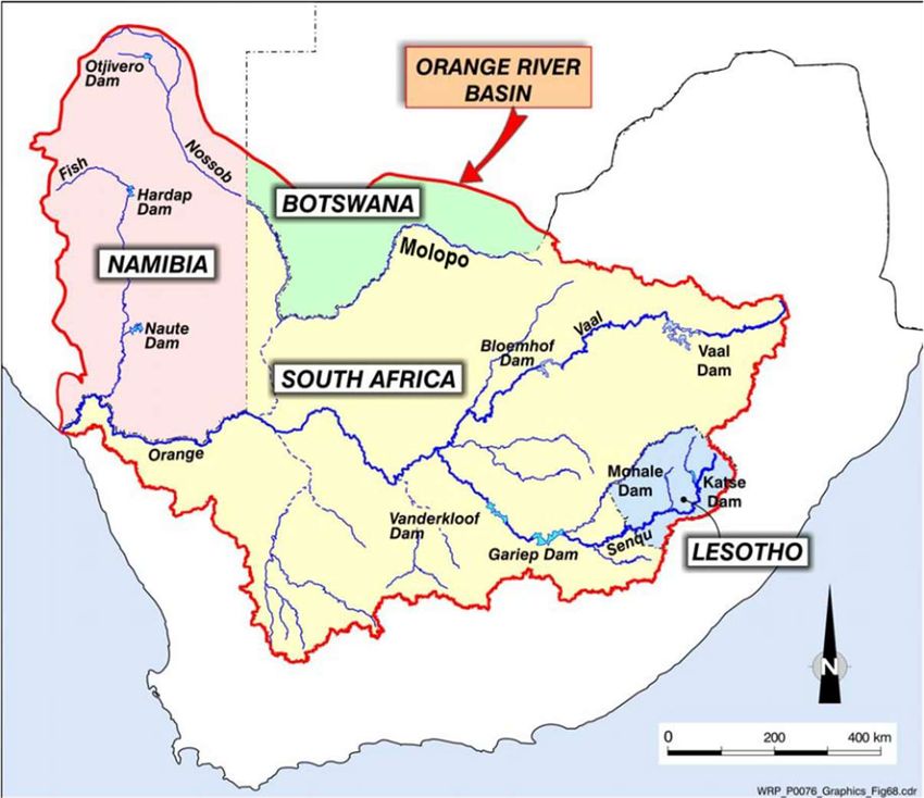
Pahlow et al. (2015), the Orange river basin suffers from water scarcity for 6 months of the year,
without even including the blue water footprint of reservoirs and water transfers. This shows the need
for BWCs if the policymakers wish to preserve the environment. The National Water Act (NWA, No. 36
of 1998) (RSA, 1998) describes the ultimate aim of water resource management is achieving
sustainable use of water for the benefit of all users and made aquatic ecosystems along with basic
human needs the only two sectors with a legitimate right to their water, making this portion an
untouchable reserve.

 1.4. Research questions
From the objective, the main research question is derived.

 How can monthly blue water footprint caps for the Orange river basin be formulated and how
 can reservoir management influence these caps?

This research question will be answered by answering the following sub research questions which
indicate the process steps.

 1. What is the historical monthly runoff in the Orange River and has it changed over time?
 2. What are the environmental flow requirements in the Orange river?
 3. What is the blue water footprint within the Orange River and to which extent does it
 violate the environmental flow requirements?
 4. How can monthly blue water caps be formulated?
 a. How can monthly BWCs be set per sub-catchment?
 b. What is the effect of reservoirs on a BWC?

 1.5. Scope
In this paragraph, the scope of the thesis will be discussed. First of all, within the water footprint
framework, the focus will lie on blue water and not on grey and green water. The water footprint caps
are set on a monthly time step rather than on an annual basis. In this way, the often great intra annual
variability of water supply and use throughout the year is incorporated.

 1.5.1. Geographical boundaries
The Orange River is named by Colonel Robert J. Gordon, in honour of the Dutch Prince of Orange. It
rises at 3200 m AMSL in the Drakensberg Mountains and high plateau of Lesotho, where it is called the
Senqu, and flows west with an average gradient of 1.4 / about 2300km to the Atlantic Ocean at
Alexander Bay. It passes from cool-temperate and moist alpine regions to progressively more arid
terrain of the west Atlantic coast. The Orange is the largest river system in Africa south of the Zambezi,
with a catchment of 650 000 km2 (Cambray et al., 1986).

The Orange River (Figure 2) is transboundary, it covers Lesotho, South Africa, Namibia and Botswana.

 3

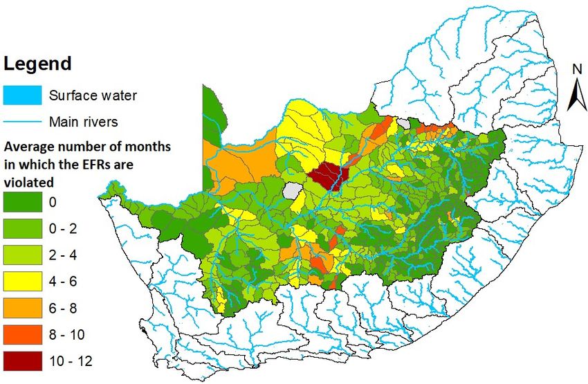
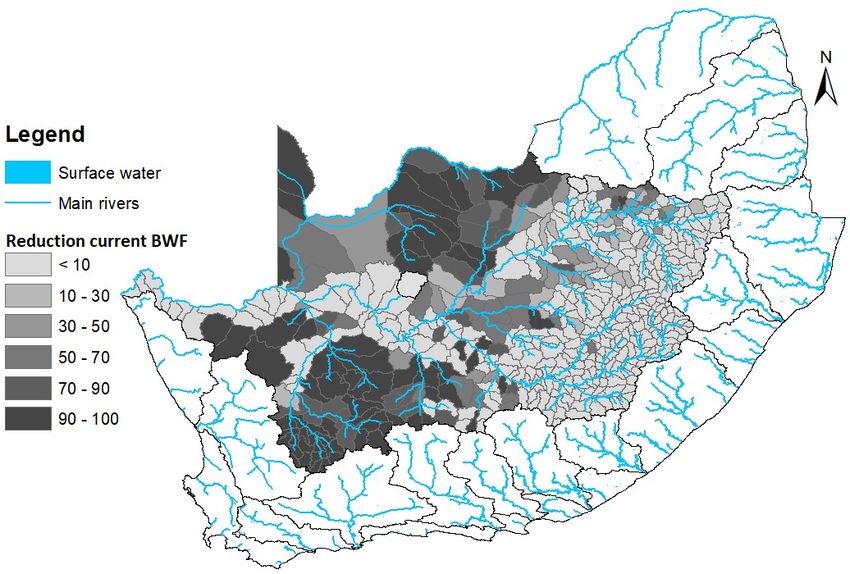
Figure 2: Orange river basin (Orasecom, 2007)

There is some debate whether the Molopo and the Nossob river belong to the Orange River basin. The
Molopo river is suspected to historically have contributed runoff to the Orange river (Matthews, 2015).
Currently, it is blocked by dunes from the Kalahari desert downstream the confluence of the Nossob
river, meaning that surface runoff is unable to reach the Orange River (Heyns, 2003). Water from these
rivers might still reach the Orange river through groundwater flows (Heyns, 2003) and the fact that this
landscape is dynamic means that these dunes might have moved since 2003. This thesis will follow the
current literature (Lange et al., 2007; Orasecom, 2007; Orasecom, 2010) and include the Molopo and
Nossob river as part of the Orange River basin.

The most recent water resource study of South Africa, Water Resources of South Africa (2012), did not
include Botswana and Namibia. A different study about the Orange River basin by Orasecom (2010)
did include Botswana and Namibia but did not openly share their data. Therefore the study area has
been to Figure 3. This means that runoff from Botswana and Namibia which contribute

Figure 3: Study area of the Orange River which lies within South Africa and Lesotho

Endorheic areas fall outside the study area as they are not considered part of the Orange River basin
and both runoff and EFR data were not available (Orasecom, 2010; Water resources of South Africa,
2012). This does not mean that people living in endorheic areas cannot consume any water. Specific
environmental studies have to be performed for these areas, which could result in a certain lake or
groundwater level being required for the environment.

 1.5.2. Terminology
In this paragraph the used terms and abbreviations during this research are defined, this terminology
is in line with the terminology used in the water footprint assessment manual (Hoekstra et al., 2011).

 Definition Abbreviation Description Unit
 Blue water BW Fresh groundwater and surface Million m3 per month
 water
 Blue water BWF A measure of humanity’s Million m3 per month
 footprint appropriation of blue water
 Blue water BWA This is the maximum sustainable Million m3 per month
 availability amount of water which can be
 consumed.

 Blue water BWC A set amount of water that is Million m3 per month
 footprint cap allowed to be consumed in a
 water allocation policy.
 Environmental EFR Runoff required for the Million m3 per month
 flow requirements preservation of the environment

 Local runoff Runoff locally generated within a Million m3 per month
 catchment
 Present-day Modelled runoff with land-use Million m3 per month
 runoff set to the situation of 2010
 Historical runoff Modelled runoff with historical Million m3 per month
 land-use estimation
 Natural runoff Modelled runoff under natural Million m3 per month
 conditions, no human influences
 are taken into account

 5

Actual runoff Estimated actual river flow, Million m3 per month
 Historical runoff with human
 influences included.

In Figure 4 a flow chart is given which shows how the research questions are related to each other.

Figure 4: flow chart of how the different steps leading towards answering of the research questions

 6

2. Theoretical framework
In this chapter, the theories and existing models regarding the research questions are discussed.

 2.1. Monthly runoff in the Orange river
Because of the large intra annual variability, the choice is made to set the BWCs on a monthly time
scale as water shortage in one month cannot be crossed against the abundance of water in another
month (Hoekstra, 2013). This gives the first requirement: The runoff should be determined on at least
a monthly time scale. The second requirement has to do with the spatial resolution. Hogeboom et al.
(2020) have set monthly BWCs for the entire Orange River basin, but ideally they are set on the level
of sub-catchments (Hoekstra, 2013), as water shortage in one tributary cannot be crossed against
water abundance in another tributary. This means the runoff should be determined on the grid level
or small sub-basins. The last requirement has to do with the influence of humans. To determine EFRs,
natural runoff needs to be known. This means runoff has to be estimated which excludes human
influences.

The amount of runoff can be either observed or modelled. Since BWCs will be set per sub-catchment
and runoff has only been measured at a few locations, the runoff will have to be modelled. Runoff can
be modelled in many different ways. Rainfall-runoff models are classified based on model input and
parameters and the extent of physical principles applied in the model (Devia et al., 2015). The structure
of a model determines how it calculates runoff. Hydrological models are generally sorted into three
categories: Empirical, conceptual and physical models. Physical models require much more data than
there is available and conceptual models are regarded as more detailed than empirical models (Devia
et al., 2015). The Pitman (1973) conceptual rainfall-runoff model is chosen because it is specifically
designed for South Africa and has over the past 46 years become one of the most widely used
hydrological models in southern Africa (Hughes, 2013). It is chosen instead of global hydrological
models because calibrated conceptual models based per sub-catchment are considered as more
detailed than global hydrological models (Zhang et al., 2016).

 2.2. Environmental flow requirements in the Orange river
Freshwater ecosystems provide a range of goods and services for humans, including fisheries, flood
protection, wildlife, etc. (Acreman, 2001; Revenga et al., 2000). Water needs to be allocated to these
ecosystems to maintain them. Balancing the requirements of the aquatic environment and other uses
is becoming critical in many of the world’s river basins as population and associated water demands
increase (Vörösmarty et al., 2000). Meanwhile, the assessment of the EFRs is also a major challenge
due to the complexity of physical processes and interactions (Smakhtin et al., 2004). Environmental
flows are defined in the Brisbane declaration (2018): “Environmental flows describe the quantity,
timing, and quality of freshwater flows and levels necessary to sustain aquatic ecosystems which, in
turn, support human cultures, economies, sustainable livelihoods, and well-being.” There are multiple
methods to determine the environmental flow requirements (EFRs) of a river. These methods are
categorised in four categories: Hydrological methods, hydraulic methods, habitat simulation methods
and holistic methods (Tharme, 2003).

Holistic methods are methods which combine hydrological, hydraulic and ecological data in
combination with experts to estimate site-specific EFRs. These methods are generally assumed to best
estimate the ecological needs of a river (Pastor et al., 2014; Tharme, 2003). Holistic methods are mainly
developed in South Africa and Australia (Hughes & Louw, 2010), unfortunately the results of many
holistic EFRs studies are not available. Only one study for the Orange river basin could be found. In
2010 the following study was performed: Support to Phase II ORASECOM basin-wide integrated water
resources management plan (Orasecom, 2010). One of the main objectives of the study was to assess

 7

EFRs at key areas of the Orange River Basin. They selected six hotspots on which detailed EFR
assessments have been carried out. The process of setting EFRs in South Africa centres on the concept
that aquatic ecosystems may be maintained at different levels of condition (health). These different
classes can be seen in Table 1.
Table 1: Management classes for the environmental flow of South Africa (King et al., 2008)

The study selected different management classes for different parts of the Orange River. The assigned
management classes are set one class higher than the current state. E.g. if a river section has currently
management class D the EFRs have been determined for class C. Combining these different EFR sites
would result in river sections with negative EFRs and situations where the EFRs are impossibly met due
to lower management classes assigned upstream and a lack of locally generated runoff. Next to this,
the vision of setting BWCs is that the environment is respected, it would be strange to set a BWC based
on EFRs which still results in a high degree of modification from the natural condition.

For these reasons, the decision has been made to only use the EFR from one site. The strictest site in
the main orange river is chosen, which is EFR O3: Augrabies with management class A. This site is
located just upstream of the Fish River, the river from Namibia of which no runoff data is available.
Thus only South Africa and Lesotho are responsible for the runoff which reaches this EFR site, which
means that the Fish river can be neglected.

 2.3. Blue water footprint accounting
The water footprint is a measure of human’s appropriation of freshwater resources (Hoekstra et al.,
2011). For this study, the focus will lie on the blue water footprint which refers to the consumption of
blue water resources (surface and groundwater). The blue water footprint of production within the
Orange river basin is the sum of all water-using processes in the area (Hoekstra et al., 2011).

It is not feasible to get data on all the individual processes taking place, therefore the choice is made
to account the major processes. Hoekstra and Mekonnen (2012) have estimated the national BWF of
production in South Africa which resulted in a total blue water footprint of national production of 7123
million m3. The main contributors are crop production (90.0 %), domestic water supply (5.5 %),
industrial activities (0.5 %) and animal water supply (4.0 %). In addition to these sectors, the BWF of
reservoirs and inter-basin transfers have also been taken into account as the literature indicates that
these are major water consumers (Lange et al., 2007; Orasecom, 2007). Inter-basin water transfers do
not consume water themselves, but water is taken out of the Orange river basin and is not returned.
Hoekstra et al. (2011) state: ‘The export of real water out of an area, as in the case of an inter-basin
transfer, will be counted as a process water footprint in the area from which the water is exported’.
No spatial data was available of the location of farm animals within the orange river, thus this BWF has
been left out. Which leaves the following sectors as blue water consumers:

 8

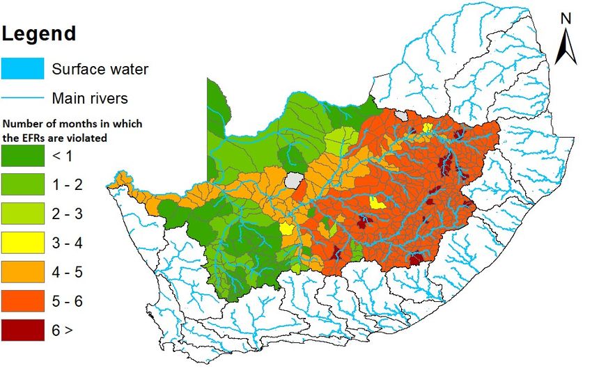
 Production of crops
  Domestic water supply
  Industrial water supply
  Reservoir evaporation
  Inter-basin water transfer

 2.4. Environmental sustainability of the blue water footprint
To assess the environmental sustainability of the current BWF, environmental sustainability has to be
defined. Hoekstra et al. (2011) state ‘When, in a certain month, the blue water footprint within a
catchment exceeds the blue water availability, the blue water footprint is environmentally
unsustainable, because the environmental flow requirements are violated.’ Therefore to assess the
environmental sustainability the number of times in which the EFRs are violated per sub-catchment is
analysed.

Hoekstra et al. (2011) identified a second criterion to analyse the effect the BWF has on groundwater
and lake levels in a catchment. the blue water scarcity is defined by Hoekstra et al. (2011) as follows:
 ∑ [ , ] (1)
 [ , ] =
 [ , ]
There are some flaws to this criterion identified by Pellicer-Martínez and Martínez-Paz (2016), which
make it unable to be used as interpretation of the results becomes meaningless. First, it is unable to
cope with zero and negative values of BWA. This becomes especially problematic when analysing the
criteria spatially. To give an example for a downstream sub-catchment with no local runoff and
upstream users who used the maximum sustainable amount of water. The inflow is 100 units of water,
the BWF is 1 unit of water and the EFRs are 100 units of water. This would result in a water scarcity
value of infinite. Does this mean that this catchment is infinitely depleting the groundwater stocks and
lake volumes? No, because the actual EFRs are only violated for a mere 1 %. Second, it is unknown how
reservoir management should be taken into account. A reservoir increasing its storage can be seen as
either as a water consumer or a reducer of the BWA, which result in different values.

Wada et al. (2011) use a different definition of water scarcity, they neglect EFRs and use average
monthly values for runoff and demand. Neglecting EFRs and inter annual variability means that also
this criterion cannot be used for the assessment of environmental sustainability.

Pellicer-Martínez and Martínez-Paz (2016) propose a new indicator, called the environmental blue
water scarcity. This indicator is obtained by comparing the environmental flow required [ , ] with
the actual runoff _ [ , ] in time interval t.

 [ , ] (2)
 _ [ ] = [ ]
 _ [ , ]

If the _ [ ] is above one than the environmental flow requirements in sub-catchment J are
not met and is regarded as unsustainable. This is a somewhat crude way of making the water scarcity
indicator set by Hoekstra et al. (2011) spatially applicable. Taking the maximum value means the results
will only reflect the worst moment in a time series, which makes it dependent on the length of the
analysed period. Modelled runoff combined with historical BWF and reservoir storage data will result
in some bad model discrepancies, where the modelled actual runoff is very or low or high compared
to observed runoff. Hence this indicator will probably bring forward the data inconsistencies. Pellicer-
Martínez and Martínez-Paz (2016) also differentiate between environmental demand and
environmental flow, but it is unclear how they define these terms.

 9

The choice is made to regard the added value of these different water scarcity indicators as
neglectable, therefore sticking to the original definition by Hoekstra et al. (2011) of sustainability and
analysing the frequency of an unsustainable situation. Besides a new indicator is proposed which can
analyse the severity of EFR violation.

 2.5. Formulating potential BWCs per sub-catchment
The idea of setting BWCs has only been explored by two studies so far (Hogeboom et al., 2020; Zhuo
et al., 2019). Zhuo et al. (2019) divide the Yellow River basin into three sections, which is similar to
dividing into sub-catchments but does not take into account the temporal variability in runoff.
Hogeboom et al. (2020) do take temporal variability into account by setting BWCs on different
percentiles of BWA for entire river basins, allowing for some accepted violation of the EFRs to utilize
potential sustainable water consumption.

 2.6. BWC allocation
If BWCs were to be set solely based on the locally generated runoff, then water is distributed based on
the source. This would imply that downstream areas which depend completely on river flow from
upstream would be without water. For this reason, an allocation method has to be implemented to
distribute water in a fair and equal way. The Global Water Partnership defined Integrated Water
Resource Management as a “process which promotes the coordinated development and management
of water, land and related resources, in order to maximize the resultant economic and social welfare in
an equitable manner without compromising the sustainability of vital ecosystems” (Global Water
Partnership, 2000). Previously the sustainability part has been assessed. The allocation of water to
maximize the resultant economic and social welfare in an equitable manner will be discussed by first
looking at the concept of ‘equity’ in water allocation and next to the maximization of the economic
and social welfare.

 2.6.1. Equity
Rasinski (1987) defines two factors which describe equity of distribution of a resource in the context
of social welfare, ‘proportionality’ and ‘egalitarianism’. Proportionality implies that resources should
be distributed according to people’s effort or ‘deservedness’. Egalitarianism suggests that everyone
should be treated equally (Rasinski, 1987). When looking at equity in the context of water resource
management, Gleick (1998) defines equity as: ‘a measure of the fairness of both the distribution of
positive and negative outcomes as well as the process used to arrive at particular social decisions.’
Cremers et al. (2005) even distinguish five levels of equity for water management at the local level:
‘equitable water distribution and allocation among different water users and uses; equitable
distribution of the services involved in irrigation development; equitable distribution of the added
agricultural production and other benefits under irrigation; equitable distribution of the burdens and
obligations related to functions and positions; and equitable distribution of the rights to participate in
the decision-making process.’ All these explanations of equity make it seem like a positive goal, but it
is still unclear how it can be implemented in an actual allocation strategy.

Van der Zaag et al. (2002) and Seyam et al. (2000) attempt to define measurable criteria based on
which water resources can be equitably allocated to the riparian countries. They try to calculate each
countries equal share or ‘right’ by applying different allocation strategies. The allocation strategies are
based on population size, surface area and locally generated blue and green water. The strong points
of these algorithms are that they are very simplistic and simple to understand. Weak points are that
they fail to grasp spatial and temporal variability (Seyam et al., 2000; Van der Zaag et al., 2002).

The algorithms of Seyam et al. (2000) and Van der Zaag et al. (2002), do not allow for any storage or
release of water as the algorithm only considers a single time step. If these algorithms were to be used

 10

to set monthly caps, the 12 months of a year have to be seen independent from one another, which is
not the case when reservoirs are included. Reservoirs are vital in the distribution of water and have to
be part of an allocation strategy. This is the most important argument against the use of these
algorithms. A second argument against the appliance of these algorithms on the level of sub-
catchments is that the criteria which seem to resemble equity between competing countries do not
resemble equity on the level of sub-catchments. E.g. allocation based on the surface area does not
seem equitable for a small sub-catchment with a large city, on the other hand, allocation based on
population size can limit the sub-catchments which are very dependent on their agricultural sector.

For the basin level, Wolf (1999) argues that equity is ‘a vague and relative term in any event. Criteria
for equity are particularly difficult to determine in water conflicts, where the international water law is
ambiguous and often contradictory’. Hence instead of defining equity, Wolf shows different
approaches currently utilized on the international level, but it is debatable whether these approaches
are in fact ‘equitable’ or just convenient for two or more parties sharing the basin. Wegerich (2007)
concludes on his research on equity in the Amu Darya basin that: ‘Even though a quest for equity is
popular at the current time in the water policy debate, the discussion on equity has shown that equity
is an ambiguous concept. For example a policy intention to establish equity on one matter might imply
inequity on a different matter (equity of inputs could lead to inequity of outputs)’. Young (1995) even
argues: ‘The arguments against existence (of equity) take three different forms. The first is that equity
is merely a word that hypocritical people use to cloak self-interest – it has no intrinsic meaning so
therefore fails to exist. The second – is that even if equity does exist in some national sense, it is so
hopelessly subjective that it cannot be analysed scientifically – it fails to exist in an objective sense. The
third argument that there is no sensible theory about it – thus it fails to exist in an academic sense.’
The literature above (Seyam et al., 2000; Van der Zaag et al., 2002; Wegerich, 2007; Wolf, 1999) already
shows that equity can be analysed scientifically and therefore exists in an academic sense proving
Young (1995) wrong.

Farriansyah et al. (2018) do asses equity for a water allocation problem on a river basin represented
by network nodes including reservoirs similar to the one in this thesis. Farriansyah et al. (2018) assess
equity by setting the percentage of which the current demand is met at each node equal. This
percentage is evaluated at the most downstream node and lowered if not enough water is available
here. This gives some level equity in their example because the total demand cannot be met by the
available water and the EFRs are set on 5% of actual runoff and thus always met. Applying this method
together with the EFRs set in this thesis would result in some level of equity, but it would reduce the
size of the BWC further than necessary for the EFRs. Not using available blue water just for the sake of
treating everybody equally is similar to telling a country not to use its natural resources, because its
neighbour doesn’t have any resources either. Also, Farriansyah et al. (2018) do not differentiate
between different sectors. A similar water availability model WRAP (Wurbs, 2005) mentions nothing
about equity in water allocation, the CWAM allocation model (Wang et al., 2008), does allow for equity
and non-equity constrains but fails to mention how these could look like.

Although some attempts have been made to specify ‘equity’ in water allocation management
(Farriansyah et al., 2018; Syme et al., 1999; Van der Zaag et al., 2002), none provide a way to define
equity and show how an allocation strategy can be designed which promotes efficiency, equity and
sustainability. As Wegerich (2007) concluded that ‘equity’ is always an ambiguous concept, therefore
difficult to analyse scientifically. To give a typical example for South Africa, assumed that the
agricultural BWF has to be reduced to meet the environmental regulations. One could argue that the
least water-efficient farmers should reduce their water consumption as they proportionally bring the
least economic welfare in euro per unit water. On the other hand, these are often the poor black

 11

farmers who do not have the money to buy modern equipment, taking away their water is not
regarded as equitable.

For this thesis, the concept of ‘equity’ is left for the actual policymakers as it will always be an
ambiguous concept. Wolf (1999) also argues that other policy instruments can be used to achieve
equity besides the allocation strategy, such as taxes on water consumption and compensations. For
now, the focus will lie on the maximisation of the resultant economy and social welfare without
compromising the sustainability of vital ecosystems.

 2.6.2. Maximisation of the resultant economy and social welfare
Maximisation of the resultant economy and social welfare is more straightforward. Many articles do
this by assigning an economic value to every aspect of the allocation strategy (Rosegrant et al., 2000).
They then sum the economic value of every aspect (e.g. consumption of sectors, hydropower benefits
of reservoirs or lake levels for recreational purposes.) resulting in a price of what a certain allocation
strategy is worth.

Maximisation of the economic value requires an optimization technique (Zhu & Van Ierland, 2012).
Optimization is difficult due to the spatial variability of BWA. Downstream consumption means that
upstream consumption has to be limited, but it is difficult to determine which upstream sub-
catchments should limit their consumption. In literature, this is solved by applying numerical
optimisation techniques (Divakar et al., 2011; Farriansyah et al., 2018; Ringler, 2001). Applying an
optimisation algorithm consists of four components:

  Objective function
  Set of parameters to be optimized which determine the objective
  Boundary conditions
  Selection of an optimisation algorithm

How this will be implemented will be further discussed in paragraph 3.4.

 12

3. Methodology
In this chapter, the methods used to answer the research questions are described and discussed.

 3.1. Estimating historical runoff
The latest water resource study by Royal HaskoningDHV has provided calibrated parameters for the
WRSM/Pitman model for 1944 sub-catchments of South Africa of which 479 are located within the
Orange river basin (Water Resources of South Africa, 2012). This model in combination with monthly
rainfall data results in monthly runoff data per sub-catchment from 1920 through 2010. The model can
be simulated with different settings for the paved area, alien vegetation and afforestation, which
results in the following three types of runoff.

  Natural runoff would occur without the man-made influences such as dams, irrigation
 schemes, abstractions for mines, industry and towns, return flows from treatment works, etc.
 This natural runoff has been simulated by disabling: paved areas, afforestation and alien
 vegetation.
  Present-day runoff would occur with the most recent land use. The model has thus been
 simulated with paved area, afforestation and alien vegetation set to the situation of 2010
 (which is the most recent land-use setting) with historical rainfall.
  Historical runoff would historically have occurred without abstractions and has been modelled
 with historical estimated paved area, afforestation and alien vegetation.

Data on the runoff direction from the sub-catchments, which sub-catchment flows into which other
sub-catchment, has been retrieved with SPATSIM (Spatial and Time Series Modelling) from the
National V2 databank of South Africa (SPATSIM, 2019). This data has been transformed into a river
network tree Figure 5. Each node represents a sub-catchment, this representation is used to properly
account the flow accumulation from upstream to downstream.

Figure 5: Tree structure of a river with each node being a sub-catchment and with the flow direction from right to left

At each node the following mass balance equation is used:

 − = Δ (1)
Where is the inflow, which is the locally generated runoff plus inflow from an upstream sub-
catchment. is the outflow which is water consumed in the sub-catchment plus outflow to a
downstream sub-catchment. Δ is the change in storage in the sub-catchment. Δ = 0 at all the
catchments without a reservoir (Figure 6).

 13

Figure 6: input-output balance at a network node (sub-catchment)

There are 3 water transfer entering the Orange River, 2 leaving the Orange River and 1 intra-basin
transfer. Water transfers change the network structure of the river, a normal sub-catchment has only
one downstream sub-catchment while a sub-catchment with an intra-basin transfer has two
downstream sub-catchments and the sub-catchment of which receives water can no longer be
considered most upstream. An inter-basin transfer entering the Orange river basin is seen as inflow
from upstream. The inter-basin transfers out of the Orange river are regarded as consumers. Data on
water transfers is retrieved from Water Resources of South Africa (2012).

Figure 7: The effects of water transfers on the river network schematic

 3.1.1. Climate change analysis
The influences of climate change on the historical runoff are analysed to determine the required length
of the historical runoff used for the forecast of future runoff. If the climate has changed a lot then
runoff from 1920-1930 will probably not resemble future runoff. On the other hand, the used historical
period should be as long as possible as an increased sample size means more inter annual variability is
included. Natural runoff is used because human influences (except their influences on the climate)
have to be excluded.

Meng et al. (2016) distinguish three factors to determine the effects of climate change on historical
runoff. The total amount of runoff, the shape of the flow peak and the timing of the flow peak. Change
in the total amount of runoff is analysed by analysing the yearly runoff and the decade mean runoff
for the entire Orange River basin to limit the inter-annual variability (Meng et al., 2016). The shape of
the flow peak is analysed by looking at the intra-annual variability of the runoff. If the intra-annual
variability is low then the flow peak is smooth, if the intra-annual variability is high then the flow peak
is steep (Meng et al., 2016). The intra-annual variability has been determined by taking the standard
deviation of the runoff. Lastly, the timing of the flow peak has been determined by analysing the month
in which the maximum monthly runoff occurred and drawing a trendline through these months to see
if the timing has changed (Burn, 1994; Meng et al., 2016).

 14

3.2. Environmental flow requirements
Data on EFRs has been retrieved from Orasecom (2010) and were provided in the format of a flow
duration curve table together with a natural flow duration curve table, an exemplary month is plotted
in Figure 8. The environmental flow study uses several older natural runoff model outputs for several
sections of the Orange river (Orasecom, 2010). Different hydrological models will give different results,
for this reason, a check is performed whether the natural runoffs used are comparable. This check is
performed in Appendix A by transforming the natural runoff from paragraph 3.1 to monthly flow
duration curves.
 Natural runoff (million m3 )

Figure 8: The provided environmental flow requirements for the Orange River basin upstream of the Fish river for May in the
format of a flow duration curve (fdc), management class A stands for negligible modification from natural conditions.

The flow duration curves from the natural runoff of paragraph 3.1 and the natural runoff used by the
consultancy for their environmental flow study are similar (Appendix A). The next step is to implement
the EFRs. The EFRs are linearly interpolated to estimate the EFRs between the table values given. The
environmental flow requirements are based on natural river flow. To transform this data to
environmental flow requirements per sub-catchment the following procedure is used for the full
duration of the data series.

  The total natural runoff for the Orange river is calculated by summing the natural runoff from
 all the sub-catchments.
  For the total monthly natural runoff, the EFRs are selected which belong to the amount of
 runoff, e.g. in Figure 8, the EFRs for runoff of 600 million m3 in May are 231 million m3.
  This environmental flow is evenly spread out over the sub-catchments based on the amount
 of natural runoff which each sub-catchment contributes to the total natural river flow
 (equation 3).
 [ , ] (3)
 [ , ] = [ ]
 [ ]

Where is the EFRs retrieved from Orasecom (2010), the locally generated
natural runoff and the natural runoff at the river mouth. A downside of this procedure is
that no difference is made between regions with a different hydrological regime or different ecology,
also the table does not provide EFRs data for flow peaks which occur less than 10% of the time. For
this reason, the EFRs have been compared with the variable monthly flow method (Pastor et al., 2014)
for a dry downstream sub-catchment and a wet upstream sub-catchment to see if the results are
comparable.

 3.2.1. Variable monthly flow method
Pastor et al. (2014), developed a parametric method: The variable monthly flow (VMF) method. This
method follows the natural variability of river discharge by defining EFRs on a monthly basis. The VMF

 15

method adjusts EFRs according to the flow season. The VMF method is developed to increase the
protection of freshwater ecosystems during the low-flow season with a reserve of 60% of the monthly
mean flow and a minimum flow of 30% during the high-flow season.
Table 2: Environmental flow requirements computed with the variable monthly flow method (Pastor et al., 2014).
 Requirements Description
 High flow Runoff > 0.8 * Runoffyear, avg
 High flow requirement EFR = 0.3 * Runoff
 Intermediate flow Runoff < 0.8 * Runoffyear, avg
 Runoff > 0.4 * Runoffyear, avg
 Intermediate flow requirement EFR = 0.45 * Runoff
 Low flow Runoff < 0.4 * Runoffyear, avg
 Low flow requirement EFR = 0.6 * Runoff

 16

3.3. Environmental sustainability of the historical blue water footprint
The environmental sustainability for the period of 1990-2010 will be analysed. This is done by
accounting the BWF, furthermore the historical reservoir management has to be included to determine
the actual runoff. Lastly, this actual runoff has been compared with the EFRs to determine the
environmental sustainability of the BWF.

 3.3.1. Blue water footprint accounting
The total BWF in the Orange River basin can be described with the equation below:

 = + + + (4)
 + 

The BWF of crop production was obtained from Hogeboom, et al (in review), who estimated the
monthly global water footprint for crops on a 5 by 5 arc minute spatial resolution. This data is summed
over the area of the sub-catchments giving the BWF of crops per month per sub-catchment. Summing
the grid values over the sub-catchment is done with the ArcGIS zonal statistics tool. This results in
monthly BWF of crops in million m3 per sub-catchment.

The water footprints related to industrial production and domestic water supply were estimated by
using water withdrawal data from the AQUASTAT database (FAO, 2016). Assumed is that of water
withdrawn for industrial purposes 5% is actual consumption and that the remaining fraction is return
flow (Mekonnen & Hoekstra, 2011). For the domestic water withdrawn, 10% is assumed as actual
consumption (Mekonnen & Hoekstra, 2011). The water footprints related to industrial production and
domestic water supply were mapped using population maps. A spatial distribution map of the
population in 2010 for South Africa and Lesotho were used (Worldpop, 2018).

Underlying assumptions in this methodology are:

  The industrial BWF is spread based on population, this choice is made as the industry tends to
 be located around towns and cities (Kemper & Schmenner, 1974).
  No distinction in BWF between poor and rich people (even when South Africa is one of the
 world’s most unequal countries), but this choice is made as the impact of the domestic BWF is
 estimated to be minor.

The domestic BWF varies throughout the year (LAO, 2017) for this reason the domestic yearly BWF has
been multiplied by an urban monthly water consumption trend. The trend used is the inverse of a
trend of California (LAO, 2017), the inverse because South Africa and Lesotho lie in the southern
hemisphere. The industrial BWF is assumed to be constant throughout the year. In the tables below
are the withdrawal data retrieved from AQUASTAT (FAO, 2016).
Table 3: South Africa's water withdrawal (FAO, 2016)
 1990 1995 2000 2017
 Industrial water 1.448 1.102 1.052 4.100
 withdrawal (109 m3/year)
 Municipal water 2.281 3.092 3.904 3.890
 withdrawal (109 m3/year)

Table 4: Lesotho's water withdrawal (FAO, 2016)
 1987 2000
 Industrial water
 withdrawal (109 m3/year) 0.011 0.020

 17

Municipal water
 withdrawal (109 m3/year) 0.011 0.020

The above water withdrawal data is linearly interpolated for the years 1990 to 2017 for South Africa
and for the years 1987 to 2000 for Lesotho. For Lesotho, it is assumed that the water withdrawal
increases with the same ratio as the population increases for the period of 2000-2010 (Worldpop,
2018), to provide monthly BWF data from 1990 through 2010.

Hogeboom et al. (2018) determined that the BWF of a reservoir has both an operational and a supply
chain component. The supply chain component will not be determined as this falls under the industrial
BWF and double counting should be avoided. The operational component is calculated as follows:

 = 10 ∗ ∗ (5)
Where BWF of reservoirs is determined in per month, A is the surface area in ha and the depth
of water that evaporates per month in mm. Monthly surface areas of reservoirs have been provided
by the Department of Water and Sanitation (2019). To estimate the evaporation of reservoirs, the
same potential evaporation is used as the hydrological model uses, which is determined by pan
evaporation measurements multiplied by pan factors (Water Resources of South Africa, 2012). This is
the Kohli and Frenken (2015) method.

Data on inter-basin water transfers in the Orange river basin is retrieved from the Water Resources
study of South Africa (2012)

 3.3.2. The influence of current reservoir management on the BWA
To analyse to which extent the BWF of 1990-2010 violates the EFRs, the historically redistributing effect
of reservoirs has to be included. The mass balance from equation 1 becomes:

 − = Δ = − (1)
Where is the storage in the next month and the storage in the current month. E.g. Δ in October
is the storage on the 1st of November minus the storage on the 1st of October.

Monthly data of reservoir storage and surface area has been provided by the Department of Water
and Sanitation of South Africa (DWS, 2019). Data was provided at a monthly resolution and the start
and end dates with the reservoir capacities are listed in appendix B. Data was available for 219
reservoirs of which 40 lie in the Orange river basin. 1 reservoir had missing records, to make the data
usable missing records op to the length of four months have been interpolated. The interpolation
method used was linearly interpolation, because of the small lengths of the missing records. This left
three reservoirs with data series outside the period of 1990-2010, which leaves 37 reservoirs with
proper data. These reservoirs have a combined storage capacity of approximately 18.8 billion m3.
FAO (2016) gathered detailed information about the dams of Africa, and summing the dam capacity
within the Orange river gave a total capacity of 20.7 billion m3. For a very large portion (90.3 %) monthly
data is thus available.
Table 5: Reservoirs which have insufficient data for a significant portion of the period 1920-2010
 Reservoir name Opening Capacity Data provided by DWS
 date (million m3) Start date End date
 C2R008 Luciana Barrage 1923 55.44 2018 2019
 C3R006 Taung Dam 1995 61.37 2016 2019
 C2R002 Johan Neser dam 1922 5.67 1920 1952
 2013 2019

 18