Effect of volcanic emissions on clouds during the 2008 and 2018 Kilauea degassing events
←
→
Page content transcription
If your browser does not render page correctly, please read the page content below
Atmos. Chem. Phys., 21, 7749–7771, 2021
https://doi.org/10.5194/acp-21-7749-2021
© Author(s) 2021. This work is distributed under
the Creative Commons Attribution 4.0 License.

Effect of volcanic emissions on clouds during
the 2008 and 2018 Kilauea degassing events
Katherine H. Breen1,2 , Donifan Barahona1 , Tianle Yuan1,3 , Huisheng Bian1,3 , and Scott C. Jamesa,
1 NASA,   Goddard Space Flight Center, Greenbelt, MD, USA
2 Universities Space Research Association, Columbia, MD, USA
3 Joint Center for Earth Systems Technology, University of Maryland, Baltimore County, MD, USA
a formerly at: Departments of Geosciences and Mechanical Engineering, Baylor University, Waco, TX, USA
 deceased

Correspondence: Donifan Barahona (donifan.o.barahona@nasa.gov)

Received: 18 September 2020 – Discussion started: 22 October 2020
Revised: 22 March 2021 – Accepted: 23 March 2021 – Published: 21 May 2021

Abstract. Volcanic eruptions in otherwise clean environ-           correlation of the model results with the satellite retrievals.
ments are “natural experiments” wherein the effects of             Overall, aerosol loading, plume characteristics, and meteo-
aerosol emissions on clouds and climate can be partitioned         rology contributed to changes in cloud properties during the
from meteorological variability and anthropogenic activi-          Kilauea degassing events.
ties. In this work, we combined satellite retrievals, reanaly-
sis products, and atmospheric modeling to analyze the mech-
anisms of aerosol–cloud interactions during two degassing
                                                                   1   Introduction
events at the Kilauea volcano in 2008 and 2018. The erup-
tive nature of the 2008 and 2018 degassing events was dis-         Aerosol emissions influence Earth’s climate both directly and
tinct from long-term volcanic activity for Kilauea. Although       indirectly. The direct effect involves scattering and absorp-
previous studies assessed the modulation of cloud properties       tion of thermal and solar radiation by atmospheric aerosols,
from the 2008 event, this is the first time such an analysis       while indirect effects involve alteration of the microphysi-
has been reported for the 2018 event and that multiple de-         cal properties and the global distribution of clouds (Boucher
gassing events have been analyzed and compared at this lo-         et al., 2013; Twomey, 1977). Both liquid and ice clouds
cation. Both events resulted in significant changes in cloud       are susceptible to aerosol emissions that can alter their mi-
effective radius and cloud droplet number concentration that       crophysical (i.e., particle size distribution and albedo) and
were decoupled from local meteorology and in line with an          macrophysical properties (liquid and ice water content, cloud
enhanced cloud albedo. However, it is likely that the effects      lifetime, and cloud fraction) (Lohmann and Feichter, 2005;
of volcanic emissions on liquid water path and cloud fraction      Boucher et al., 2013; Seinfeld et al., 2016). These effects,
were largely offset by meteorological variability. Compari-        collectively known as aerosol indirect effects (AIEs), may
son of cloud anomalies between the two events suggested a          offset a significant fraction of the warming induced by green-
threshold response of aerosol–cloud interactions to overcome       house gas emissions, yet their magnitudes are poorly con-
meteorological effects, largely controlled by aerosol loading.     strained (Boucher et al., 2013). Additionally, cloud forma-
In both events, the ingestion of aerosols within convective        tion is a complex and nuanced physical process occurring
parcels enhanced the detrainment of condensate in the upper        on scales far smaller than those resolved by climate mod-
troposphere, resulting in deeper clouds than observed under        els, and the precise feedback mechanisms influencing AIEs
pristine conditions. Accounting for ice nucleation on ash par-     across various timescales are not fully understood (Boucher
ticles led to enhanced ice crystal concentrations at cirrus lev-   et al., 2013; Klein et al., 2013; Malavelle et al., 2017; Yuan
els and a slight decrease in ice water content, improving the      et al., 2011).

Published by Copernicus Publications on behalf of the European Geosciences Union.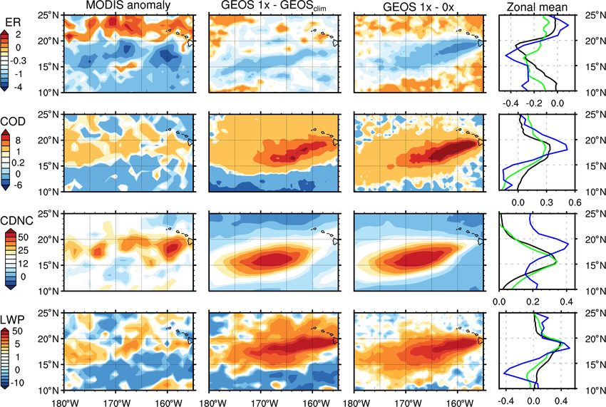
7750       K. H. Breen et al.: Effect of volcanic emissions on clouds during the 2008 and 2018 Kilauea degassing events

   The presence of cloud condensation nuclei (CCN; typi-              In this work, we assessed the effects of SO2 and ash
cally sulfates, organics, and nitrate particles) in the atmo-      aerosol emissions on liquid and ice cloud formation during
sphere indirectly impacts Earth’s net radiative balance by         two volcanic degassing events from Kilauea in June 2008
increasing the number of cloud droplets, hence altering the        and May 2018 (Fig. 1). In both of these events, atmospheric
scattering and absorption of incoming solar radiation. This        aerosol loading increased by several orders of magnitude
effect, historically referred as the first AIE or “Twomey” ef-     over a few days and remained high for at least 2 to 3 months.
fect (Twomey, 1977), represents a change in Earth’s albedo         The volcanic and seismic activity during peak emissions in
and results in net radiative cooling. Smaller droplets are also    2008 and 2018 has been well-characterized (Nadeau et al.,
less efficient at coalescing into rain-bearing clouds. Non-        2015; Neal et al., 2019; Elias and Sutton, 2012; Elias et al.,
precipitating clouds have a longer lifetime and thereby pro-       2020; Wilson et al., 2008; Orr and Patrick, 2009; Orr et al.,
vide extended coverage, which is known as the second AIE           2013; Patrick et al., 2019; Kern et al., 2020), revealing that
(Albrecht, 1989). Aerosols can also act as ice nucleation par-     emission rates of SO2 during the 2018 event were conserva-
ticles (INPs; typically dust, soot, and organics), modifying       tively at least ≥ 5× higher than 2008 peak degassing emis-
cloud properties at low temperature (Lohmann and Feichter,         sions (Kern et al., 2020; Elias et al., 2020). Analysis of the
2005). Besides these effects, CCN and INP ascend within            satellite record has shown significant anomalies in aerosol
convective parcels and determine, to a large extent, the onset     loading and liquid cloud properties during the 2008 event re-
of precipitation, modifying the release of latent heat within      sulting from volcanic emissions (Eguchi et al., 2011; Yuan
convective clouds (Koren et al., 2005).                            et al., 2011; Beirle et al., 2014), in agreement with modeling
   Satellite datasets facilitate global observational monitor-     studies (Malavelle et al., 2017). Tang et al. (2020) showed
ing of meteorology, ambient aerosol concentrations and dis-        significant effects of the 2018 Kilauea emissions on air qual-
tributions, and cloud properties. However, inferring aerosol–      ity. However, analyses of ice clouds and of the impacts of
cloud interactions (ACIs) from satellite retrievals is diffi-      the 2018 event on cloud properties and evolution have not
cult due to the concurrent influence of meteorological effects     yet been reported. This work constitutes a substantial contri-
(i.e., variation in temperature, water vapor, and winds from       bution towards identifying ACI signatures for liquid and ice
large-scale forcing) on clouds (Lohmann and Feichter, 2005;        macrophysical and microphysical processes as well as their
Gryspeerdt et al., 2017). From a modeling perspective, the         sensitivity to aerosol loadings, CCN, and INPs.
relevant scale for ACIs (i.e., tens to hundreds of meters) is         This work is organized as follows. Section 1.1 provides an
typically unresolved in atmospheric general circulation mod-       overview of each degassing event. Satellite datasets used in
els (AGCMs; Boucher et al., 2013) for which grid resolution        the analysis are described in Sect. 2, and the modeling ap-
is coarser (generally thousands of meters). The parameteriza-      proach is described in Sect. 3. Section 4 discusses the results
tion of ACIs in AGCMs is largely dependent on theory, with         of our analysis, with an emphasis on liquid and ice cloud in-
many assumptions involved, and model outputs are difficult         teractions. Finally, concluding remarks are given in Sect. 5.
to validate directly against satellite retrievals due to differ-
ences in resolution.                                               1.1   Kilauea degassing events
   Volcanic degassing events in otherwise “clean” environ-
ments, where anthropogenic aerosol emissions are minimal,          Kilauea is an active basaltic shield volcano located on the Is-
have been used as “natural” experiments to identify charac-        land of Hawai’i. Volcanic plumes on Kilauea are generally
teristics of ACIs in satellite retrievals and to evaluate AIEs     low-altitude (< 10 km) because the gentle slopes of the vol-
in GCMs. This is well-exemplified at the Kilauea volcano           cano provide little protection from strong trade winds and
(Fig. 1) in the Hawaiian Islands (Eguchi et al., 2011; Yuan        because of the shallow depth of the summit crater (< 100 m)
et al., 2011; Beirle et al., 2014; Malavelle et al., 2017). Not    (Elias et al., 2018). Since March 2008, volcanic activity on
only are local anthropogenic emissions low in the local en-        Kilauea has been marked by summit degassing and flank
vironment surrounding Kilauea, but because the volcano is          eruptions with increasing intensity and frequency (Nadeau
situated on an island approximately 1500 km from the near-         et al., 2015). Degassing events were likely triggered by rock-
est major anthropogenic emissions source (US west coast),          falls related to vent widening and/or seismic activity, which
there is a low likelihood of multiple emission sources of          then disturbed the lava lake surface, beneath which a layer of
similar magnitude; therefore, the climatic effects of volcanic     gas had accumulated (Orr and Patrick, 2009; Orr et al., 2013).
emissions may be evaluated against relatively pristine back-       Degassing events produced variable volumes of tephra (ash),
ground conditions. Kilauea has had long-term monitoring of         and some larger explosive events scattered lithic material
emissions, seismic activity, and eruptive behavior over the        (rock and ash) within a radius as large as 50 ha surrounding
historical record. Being a low-altitude volcano, Kilauea also      the vent and produced an ash-rich plume (Elias and Sutton,
provides a unique opportunity to study ACIs for liquid and         2012; Elias et al., 2020; Nadeau et al., 2015). The summit
ice cloud phases since the injection height of the emissions       of Kilauea has been in an eruptive state since 2008, and the
is mainly controlled by the strength of the eruption.              degassing events of 2008 and 2018 represent brief periods of
                                                                   increased volcanic activity and SO2 emissions, resulting in

Atmos. Chem. Phys., 21, 7749–7771, 2021                                             https://doi.org/10.5194/acp-21-7749-2021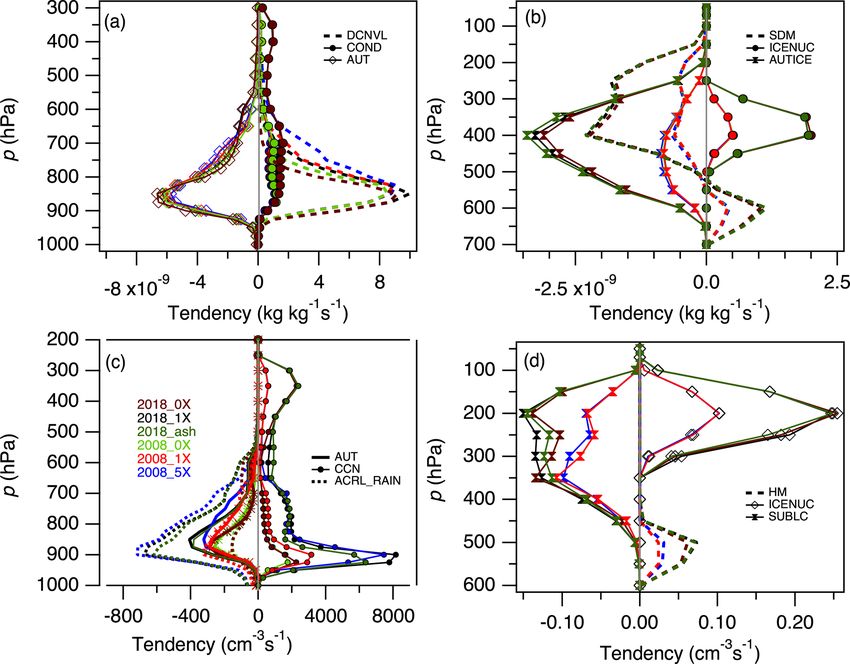
K. H. Breen et al.: Effect of volcanic emissions on clouds during the 2008 and 2018 Kilauea degassing events                      7751

Figure 1. © Google Earth imagery of the Kilauea summit crater before and after each degassing event. Clockwise from top left: pre-2008
degassing, post-2008 degassing, during 2018 peak degassing, and post-2018 degassing. The image from 5 June 2011 shows the summit vent,
which was not present prior to the 2008 event, passively degassing during an eruptive lull. The image from 30 May 2018 was taken on a
cloudy day during the 2018 event, several days after peak observed SO2 emissions (> 100 kt d−1 ) and plume height (< 8 km) (Kern et al.,
2020). The red boxes approximately outline the summit crater, while the X symbols indicate the degassing vent.

an optically denser plume relative to passive degassing. Some         tive degassing activity at the vent and longer periods of effu-
studies have noted residual effects of the plume downwind of          sive volcanism in the ERZ caused ongoing aerosol emissions
Kilauea long after violent eruptions ceased (Businger et al.,         (Patrick et al., 2019). While in 2008 most degassing occurred
2015; Pattantyus et al., 2018).                                       at the summit vent, in 2018 degassing largely occurred in
   From March to August 2008, summit activity was charac-             the ERZ and drained lava beneath the summit vent, causing
terized by degassing bursts from lava in the enlarging vent           massive deformation of the summit crater, as shown in Fig. 1
cavity and small explosive events. During degassing events,           (lower left). Additionally, the ocean entry of 2018 ERZ erup-
the estimated SO2 plume height ranged from 1200 to 2500 m             tions caused large clouds of vaporized HCl and water va-
above sea level and SO2 emissions exceeded 10 000 t d−1               por to ascend with the plume (Kern et al., 2020). Overall,
(Elias et al., 2020). Observational and modeling studies re-          the height and geologic composition of the plume in 2018
vealed a significant departure of cloud droplet size and op-          were similar to more violent, siliciclastic eruption types (i.e.,
tical thickness from their climatological values during the           Mt. St. Helens; Mastin et al., 2009); therefore, the 2018 event
2008 event, consistent with increased concentrations of at-           represented a distinct departure from long-term (decadal)
mospheric aerosols within the SO2 plume from the Kilauea              trends. Figure 1 (bottom row) shows the summit crater be-
summit crater (Eguchi et al., 2011; Yuan et al., 2011; Beirle         fore, during, and after peak eruptive activity in 2018 and in-
et al., 2014; Mace and Abernathy, 2016; Malavelle et al.,             dicates optically denser clouds within the aerosol plume with
2017). Figure 1 (top row) shows images before and after               respect to surrounding clouds during peak degassing (Fig. 1,
the 2008 degassing event. After the 2008 event, the vent can          lower right).
be seen in the SE corner of the summit crater passively de-
gassing from the lava lake during an eruptive pause.
   From May to July 2018, summit eruptions and effusive               2   Data
activity in the eastern rift zone (ERZ) were common. Sum-
mit activity ejected lithic material and ash ≈ 2000 to 8100 m         Data from NASA’s MODIS instrument and from the Cloud–
above the summit vent and SO2 concentrations were elevated            Aerosol Lidar and Infrared Pathfinder Satellite Observa-
(Neal et al., 2019; Kern et al., 2020). ERZ eruptive events           tion (CALIPSO) retrievals were used to assess both hor-
(lava fountains < 80 m) were associated with SO2 emissions            izontal and vertical cloud modification, respectively, as
of ≥ 100 000 t d−1 (Neal et al., 2019; Kern et al., 2020; Elias       done in previous studies for liquid clouds (Yuan et al.,
et al., 2018). Multiple cycles of ongoing short pulses of erup-       2011; Malavelle et al., 2017; Eguchi et al., 2011; Beirle

https://doi.org/10.5194/acp-21-7749-2021                                                Atmos. Chem. Phys., 21, 7749–7771, 2021
7752       K. H. Breen et al.: Effect of volcanic emissions on clouds during the 2008 and 2018 Kilauea degassing events

et al., 2014; Mace and Abernathy, 2016). The MODIS                Missing values were replaced with Ozone Mapping and
Aqua Aerosol Cloud Monthly Collection 6 L3 Global 1◦              Profiling Suite data (https://so2.gsfc.nasa.gov/, last access:
datasets (MYD08_M3) were acquired from the Level-1 and            15 September 2020) whenever possible; otherwise, the near-
Atmosphere Archive & Distribution System (LAADS) Dis-             est real data point was used. SO2 (cm−2 ) vertical column
tributed Active Archive Center (DAAC) (https://ladsweb.           density data were converted to emission rates (kg SO2 s−1 )
nascom.nasa.gov/, last access: 15 June 2020). Our analysis        following the approach of Beirle et al. (2014) (see their
used MODIS effective radius (Reff ; liquid, ice), cloud opti-     Fig. 6). For uncertainty quantification of OMI retrievals, see
cal depth (COD; liquid, ice), cloud water path (liquid – LWP,     Carn et al. (2016, 2017).
ice – IWP, and total – TWP), aerosol optical depth (AOD),
and cloud fraction (CF). All variables are defined in Table 1.
The MODIS cloud droplet number concentration (CDNC)               3     Methods
climatology (2003–2015) was obtained from Bennartz and
Rausch (2017). For 2018, CDNCs were calculated using              To help explain the observed changes in cloud properties dur-
the method of Bennartz (2007). Grid box mean LWP and              ing the 2008 and 2018 Kilauea degassing events and to what
IWP were calculated by scaling the MODIS product us-              these changes were sensitive, we undertook a set of AGCM
ing the retrieved liquid and ice cloud fractions, respectively.   numerical experiments (Table 2) constrained by observed
No significant differences were found by scaling using ei-        SO2 emissions (Carn et al., 2015) and by MERRA-2 (Gelaro
ther daily data (MYD08_D3) aggregated into monthly means          et al., 2017). Our objective was to generate a close repre-
(Malavelle et al., 2017) or monthly products (MYD08_M3);          sentation of the clouds formed during each event to under-
therefore, monthly MODIS products were used in the analy-         stand how aerosol emissions impacted cloud microphysics
sis. MODIS anomalies were calculated as the 3-month aver-         and evolution.
age during peak degassing minus the long-term mean (2003–
2015, excluding 2008). Missing values in MODIS data, pri-         3.1    GEOS model description
marily found in CDNC and ice products, were smoothed us-
ing cubic spline nearest-neighbor interpolation and a Gaus-       The NASA Global Earth Observing System (GEOS) ver-
sian filter. Uncertainty of MODIS retrievals is discussed in      sion 5 was used to analyze and understand the observed mod-
Hubanks et al. (2015), Bennartz (2007), and Bennartz and          ifications to cloud properties during the 2008 and 2018 Ki-
Rausch (2017) (the latter is for CDNC only).                      lauea events (Barahona et al., 2014; Molod et al., 2015).
   Vertical cloud fraction profiles from the GCM-Oriented         GEOS consists of a set of components that numerically rep-
Cloud CALIPSO Product (CALIPSO-GOCCP) were ob-                    resent different aspects of the Earth system (atmosphere,
tained for comparison with model results. The CALIPSO-            ocean, land, sea ice, and chemistry), coupled following the
GOCCP dataset is developed with CALIPSO L1 data at                Earth System Modeling Framework (https://gmao.gsfc.nasa.
full horizontal resolution (330 m) and vertical resolution        gov/GEOS_systems/, last access: 10 August 2019). For this
typical for most GCMs (40 levels; 1z = 480 m) (Chepfer            work, the AGCM configuration of GEOS was used. Atmo-
et al., 2010). Instantaneous profiles of the lidar-scattering     spheric transport of water vapor, condensate and other trac-
ratio are computed and used to infer the vertical and hor-        ers, and associated land–atmosphere exchanges were com-
izontal distributions of cloud fraction. The seasonal mean        puted explicitly, whereas sea ice and sea surface tempera-
uncertainty (2006–2008) for GOCCP cloud fraction is ≤             ture (SST) were prescribed as time-dependent boundary con-
0.05 above the boundary layer (Chepfer et al., 2010). The         ditions (Reynolds et al., 2002; Rienecker et al., 2008).
dataset may be used for comparison either directly to AGCM           Transport of aerosols and gaseous tracers such as CO was
output or to AGCM and lidar simulator output, and it is           simulated using the Goddard Chemistry Aerosol and Radi-
comparable to other standard cloud fraction climatologies         ation model (GOCART) (Colarco et al., 2010), which inter-
(Chepfer et al., 2010). Comparisons between MODIS Col-            actively calculates the transport and evolution of dust, black
lection 6 and CALIPSO show agreement between MODIS                carbon, organic material, sea salt, and SO2 . Dust and sea salt
cloud-phase partitioning and CALIPSO column-wise cloud            emissions are prognostic, whereas biomass burning and an-
profiles (Marchant et al., 2016). GOCCP was used primarily        thropogenic emissions of SO2 , black carbon, and organic car-
to assess anomalies on the vertical structure of cloud fraction   bon are obtained from the Modern Era Retrospective Reanal-
and phase partitioning during both events.                        ysis for Research and Applications Version 2 (MERRA-2)
   Volcanic SO2 emissions were constrained by observa-            dataset (Randles et al., 2017). GOCART explicitly calculates
tions from the Ozone Monitoring Instrument (OMI) on board         the chemical conversion of sulfate precursors (dimethylsul-
NASA’s EOS/Aura spacecraft (Carn et al., 2015). For Ki-           fide, or DMS, and SO2 ) to sulfate. The aging of carbona-
lauea, this dataset only provides “constant” annual SO2 emis-     ceous aerosol is represented by the conversion of hydropho-
sion rates. For the 2008 event, we replaced this dataset with     bic to hydrophilic aerosols using an e-folding time of 2 d
daily varying emissions (Carn et al., 2017; Yang, 2017).          (Chin et al., 2009). Using the evolving meteorological fields
Daily emissions for 2018 were obtained from Li et al. (2020).     from GEOS, for each time step GOCART simulates the ad-

Atmos. Chem. Phys., 21, 7749–7771, 2021                                            https://doi.org/10.5194/acp-21-7749-2021
K. H. Breen et al.: Effect of volcanic emissions on clouds during the 2008 and 2018 Kilauea degassing events                 7753

Table 1. Variable definitions and acronyms.

                      Variable                Definition                                         Units
                      ACRI_SNOW               Ice crystal accretion by snow tendency             cm−3 s−1
                      ACRL_(RAIN,SNOW)        Accretion of liquid by rain and/or snow tendency   cm−3 s−1
                      AOD                     Aerosol optical depth                              –
                      AUT                     Liquid autoconversion tendency                     cm−3 s−1
                      AUTICE                  Ice autoconversion tendency                        cm−3 s−1
                      CCN                     Cloud condensation nuclei                          m−3
                      CDNC                    Cloud droplet number concentration                 m−3
                      CF                      Cloud fraction                                     –
                      CNV_DQLDT               Total detrained condensate tendency                mg kg−1 s−1
                      COD                     Cloud optical depth                                –
                      COND                    Liquid condensation tendency                       kg−1 kg−1
                      DEP                     Ice crystal growth tendency                        cm−3 s−1
                      DCNVI                   Ice convective detrainment tendency                cm−3 s−1
                      DCNVL                   Liquid convective detrainment tendency             cm−3 s−1
                      EVAP                    Droplet evaporation tendency                       cm−3 s−1
                      HM                      Ice splintering tendency                           cm−3 s−1
                      ICENUC                  Ice nucleation tendency                            cm−3 s−1
                      ICNC                    Ice crystal number concentration                   L−1
                      INP                     Ice-nucleating particles                           m−3
                      IWP                     Ice water path                                     g m2
                      LWP                     Liquid water path                                  g m2
                      MELT                    Ice melt and/or snowmelt tendency                  kg−1 kg−1
                      NHET_IMM                Ice nucleation by immersion freezing               cm−3
                      SDM                     Ice sedimentation tendency                         kg−1 kg−1 s−1
                      SCF                     Supercooled cloud fraction                         –
                      Reff                    Effective radius                                   µm
                      TWP                     Total water path                                   g m2
                      Qliq                    Liquid mixing ratio                                mg kg−1
                      Qice                    Ice mixing ratio                                   mg kg−1
                      WBF                     Wegener–Bergeron–Findeisen process (ice)           kg−1 kg−1
                      WBFSNOW                 Wegener–Bergeron–Findeisen process (snow)          kg−1 kg−1

Table 2. Simulation experiments performed.

                          Year          Experiment name    Description
                                        2008_1×            Control simulation
                                        2008_0×            No emissions from Kilauea
                          2008
                                        2008_5×            5-fold increase in Kilauea emissions
                                        2008_PH2km         Volcanic plume height increased to 2 km
                                        2018_1×            Control simulation
                                        2018_0×            No emissions from Kilauea
                          2018
                                        2018_PH4km         Volcanic plume height increased to 4 km
                                        2018_PH4km_ash     2018_PH4km plus ice nucleation on ash particles
                          2000–2017     GEOSCLIM           GEOS climatology excepting 2008

vection (using a flux-form semi-Lagrangian method; Lin and          ternally mixed. Size distributions are prescribed for different
Rood, 1996), convective transport, and the wet and dry depo-        types using five bins for dust and sea salt and single log-
sition of aerosol tracers. The calculation of AOD is a func-        normal modes for other aerosol components (Colarco et al.,
tion of aerosol size distribution, refractive indices, and hy-      2010; Chin et al., 2009). This approach was also employed to
groscopic growth. Each aerosol type is assumed to be ex-

https://doi.org/10.5194/acp-21-7749-2021                                              Atmos. Chem. Phys., 21, 7749–7771, 2021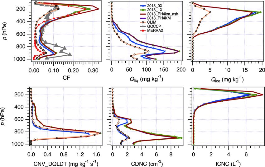
7754        K. H. Breen et al.: Effect of volcanic emissions on clouds during the 2008 and 2018 Kilauea degassing events

estimate the aerosol number concentration used in the calcu-      the climatology of the model (GEOSCLIM ). The simulation
lation of aerosol–cloud interactions (Barahona et al., 2014).     experiments are summarized in Table 2.
   Cloud microphysics in GEOS are described using a two-             To account for model drift all simulations were run in “re-
moment scheme wherein the mixing ratio and number con-            play” mode, wherein pre-computed analysis increments from
centration of cloud droplets and ice crystals are prognostic      MERRA-2 were applied to nudge the model state (i.e., hor-
variables (Barahona et al., 2014; Morrison and Gettelman,         izontal winds and temperature) to the reanalysis every 6 h.
2008). The two-moment microphysical model links aerosol           The replay technique is more stable and has lower numeri-
emissions to cloud properties and predicts the mixing ra-         cal drift than regular nudging (Takacs et al., 2018). Because
tio, number concentration, and effective radius of cloud liq-     the two-moment cloud scheme used in this work differed
uid and ice, rain, and snow for stratiform clouds (i.e., cir-     from the single-moment scheme used in MERRA-2, water
rus, stratocumulus; Morrison and Gettelman, 2008) and con-        vapor was not replayed and instead left to evolve with the
vective clouds (Barahona et al., 2014). Cloud droplet acti-       model physics. Aerosol concentrations are indirectly con-
vation is parameterized using the approach of Abdul-Razzak        strained by the reanalysis since their transport and evolu-
and Ghan (2000). Ice crystal nucleation is described using a      tion, as well as the emission of dust and sea salt, depend on
physically based analytical approach (Barahona and Nenes,         the model state (i.e., winds and temperature). The emission
2009) that includes homogeneous and heterogeneous ice nu-         of sulfate precursors (SO2 ) is constrained using satellite re-
cleation and their competition. Heterogeneous ice nucleation      trievals as described in Sect. 3.1. However, aerosol concen-
in the immersion and deposition modes follows Ullrich et al.      trations were not directly nudged to the MERRA-2 product,
(2017). Vertical velocity fluctuations were constrained by        even though the aerosol increments are also available (Ran-
non-hydrostatic, high-resolution global simulations (Bara-        dles et al., 2017). Doing so would have limited the response
hona et al., 2017). GEOS has been shown to reproduce the          of clouds to aerosol (via aerosol activation) and vice versa:
global distribution of clouds, radiation, and precipitation in    the response of aerosols to cloud formation and precipitation
agreement with satellite retrievals and in situ observations      (via scavenging). Running in replay mode ensured that the
(Barahona et al., 2014).                                          effects of meteorological variability were reduced and that
                                                                  our simulations reproduced the assimilated atmospheric state
                                                                  as closely as possible. Replaying temperature (T ) also mini-
3.2    Description of simulation experiments
                                                                  mized the role of direct and semi-direct effects in modifying
                                                                  cloud properties. Hence, our analysis focuses on the evolu-
We performed several global integrations of GEOS to best          tion of cloud microphysical properties.
isolate the effects of volcanic aerosol emissions on cloud           The altitude of the Kilauea summit crater is ≈ 1200 m,
development. Each simulation was initialized on 1 January         while the top of the well-mixed boundary layer is around
of each year and run at a nominal horizontal resolution of        2 km. For this reason, we allow the degassing volcano emis-
0.5◦ with 72 vertical levels. The time step was set to 450 s to   sions to be distributed within 1 km above the summit crater
resolve the large-scale transport of aerosol and condensate.      and constrained by the boundary layer for all 1× and 0× ex-
Cloud microphysics were subcycled twice each time step to         periments. For alternate experiments, we set an explicit
account for unresolved, fast microphysical processes such as      volcanic aerosol injection height approximating the mean
CCN activation (Morrison and Gettelman, 2008). For each           maximum plume height observed during each event (2 km
event, control runs (identified as 1×, Table 2) used the de-      in 2008; Elias and Sutton, 2012; Elias et al., 2020; Eguchi
fault model and emissions as described in Sect. 2. A sec-         et al., 2011) (4 km in 2018; Neal et al., 2019). In this work,
ond set of simulations was performed for each event, re-          we assumed that the source elevation of emissions (ERZ
moving the emissions from Kilauea (0×) to represent back-         vs. summit) was irrelevant during peak emissions but that the
ground conditions unaffected by the degassing events. Sen-        injection height of aerosols directly into the troposphere at
sitivity studies were also performed. A 5-fold actual emis-       different altitudes (below or above boundary layer processes)
sions run (2008_5×) was performed to compare the 2008 and         influenced cloud microphysics and macrophysical character-
2018 events (the 2018 event emitted ≥ 5 times the aerosol         istics for liquid and ice clouds. We also assumed the primary
load of the 2008 event) to assess the similarities between        aerosol to be SO2 with some percentage of ash, although it
the events with respect to increased aerosol loading. Sim-        is likely that sea salt contributed to ACIs in liquid clouds,
ulations to test the effect of SO2 injection height (i.e., dis-   and this is recommended for inclusion in future parameteri-
tribution of emissions constrained by plume height) on            zations.
cloud microphysics were also performed (2008_PH2km and
2018_PH4km). Finally, another numerical experiment was            3.3   Analysis method
carried out for the year 2018 (2018_PH4km_ash), wherein
the effects of ash as active INP were investigated, as de-        MODIS retrievals and the 1× GEOS experiments were com-
scribed in Appendix A. Besides these experiments, long-term       pared against the long-term climatology excluding 2008 dur-
model integration (2000–2017) was performed to represent          ing peak degassing periods for each event. The 1× simula-

Atmos. Chem. Phys., 21, 7749–7771, 2021                                            https://doi.org/10.5194/acp-21-7749-2021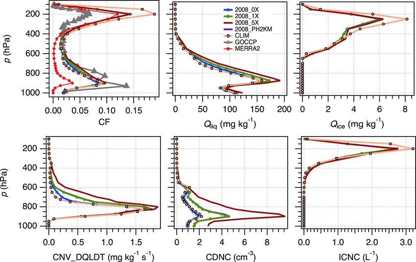
K. H. Breen et al.: Effect of volcanic emissions on clouds during the 2008 and 2018 Kilauea degassing events               7755

tions were also compared against the 0× results for each           that the effects of volcanic emissions on cloud microphysics
year (1×–0×). In this way, we assessed the effects of vol-         are specific to cloud phase. When possible, we divide the dis-
canic aerosols on cloud formation separated from natural me-       cussion between effects on ice and liquid clouds.
teorological variability. This also allowed for the assessment        Anomalies for AOD from MODIS during peak degassing
of whether passive degassing effects present in GEOSCLIM           periods are shown in Fig. 2 for JJA 2008 (top left) and
were significant contributors to ACIs as opposed to active         MJJ 2018 (bottom left). Figure 2 also shows modeled
degassing events in 2008 and 2018. The GEOSCLIM run cap-           AOD anomalies for simulations using actual emissions
tured meteorological variability, while the 0× scenario rep-       (2008_1×, 2018_1×) calculated against the simulated cli-
resents an alternative reality without volcanic emissions and      matology (GEOSCLIM ) and with zero-emissions scenarios
with the same meteorological state as the 1× runs. Correla-        (2008_0×, 2018_0×). Elevated aerosol loadings were appar-
tion between observations and the 1×–0× anomaly would              ent beginning at Kilauea (19.4◦ N, 155.2◦ W) and extended in
indicate that volcanic emissions forced ACIs that were de-         a near-Gaussian plume westward across the domain shown in
coupled from meteorology (i.e., the observed effects would         Fig. 2. AOD anomalies outside the plume domain were negli-
not have been present without elevated emissions). Con-            gible, supporting the assumption that Kilauea is located in an
versely, correlation with the GEOSCLIM anomalies would in-         otherwise “clean” environment relatively untouched by an-
dicate that the observed anomaly cannot be partitioned from        thropogenic aerosol emissions from North America or East
meteorological variability in the regional climate.                Asia. During both events, the elevated AOD anomalies ob-
   Anomalies for each degassing event were calculated as the       served by MODIS extended westward from Kilauea in the
seasonal mean during peak eruptive periods with long-term          path of the Pacific easterly trade winds (Yuan et al., 2011).
seasonal averages removed. We focused on the boreal sum-           This is well-reproduced in the GEOS results. AOD anoma-
mer (June–July–August, JJA) for the 2008 degassing event           lies appear weaker compared to GEOSCLIM than against 0×,
and the transition from the boreal spring to summer (May–          particularly near the Kilauea crater. This is due to the fact
June–July, MJJ) for 2018 when emissions from both events           that there is always some passive degassing near the source,
were highest and active eruptive events projecting ash and         which would be represented in the climatology but not in the
lithics into the volcanic plume occurred. To assess anomalies      0× experiment. Passive degassing is shown in Fig. 1, where a
at the source relative to areas outside the plume, normalized      thin plume coming from the summit crater was evident dur-
zonal mean anomalies were calculated as                            ing an eruptive pause in 2011, a year without a major vol-
                                                                   canic event at the site.
                     vlat (i)                                         Figure 3 shows MODIS retrievals and GEOS simulations
vlat,norm (i) = s                     ,                     (1)
                    N                                              of CF anomalies during the two events. Peak anomalies dur-
                          vlat (i)2
                    P
                                                                   ing the 2018 event (Fig. 3; bottom panels) were approxi-
                    i=1
                                                                   mately 2–3× greater than during the 2008 event (Fig. 3; top
where N is the number of latitudes in the domain at 5◦ in-         panels). In both cases, the 1×–GEOSCLIM difference (middle
tervals (10–25◦ N), vlat (i) is the seasonal latitudinal average   panels) reproduced the spatial distribution of the CF anomaly
(JJA 2008 or MJJ 2018) at latitude i, and vlat,norm (i) is the     from the MODIS retrieval (within the plume domain as well
seasonal latitudinal anomaly normalized by the latitudinal         as zonal means), whereas the 1×–0× differences tended
mean (JJA or MJJ averaged over the climatology) at lati-           to overestimate the anomaly in 2008 and underestimate it
tude i. To emphasize the location of the plume, we focused         in 2018. In 2008, the normalized 1×–GEOSCLIM anomaly
on a domain that included only areas west of the source (25–       correlated well with MODIS (Table 4), whereas there was
155◦ NE, 10–180◦ SW).                                              essentially no correlation between the 1×–0× anomaly and
                                                                   the retrieval, indicating that the observed CF anomaly was
                                                                   mainly driven by meteorologic variability, likely differences
4   Results and discussion                                         in SST (Takahashi and Watanabe, 2016; Boo et al., 2015).
                                                                   Thus, ACIs likely had only a minor effect on CF for the two
The goal of this work was to investigate the role of mi-           degassing events. It is possible that the aerosol layer may
crophysical processes in ACIs during the Kilauea degassing         have locally modified SST, hence indirectly affecting CF.
events. To that end, we first show the reliability of our sim-     Elucidating this requires coupled ocean–atmosphere simu-
ulations by comparing satellite retrievals and GEOS con-           lations and is suggested for future research. The discrep-
trol simulations (2008_1× and 2018_1×) and sensitivity             ancies between the simulated and MODIS anomalies were
experiments (2008_5×, 2008_PH2km, 2018_PH4km, and                  relatively larger for CF than for AOD (Figs. 2 and 3). The
2018_PH4km_ash). We then look for common features in               AOD anomalies are primarily a function of the aerosol load
both the 2008 and 2018 Kilauea degassing events and inter-         and largely determined by the volcanic events. On the other
pret their differences. Finally, Sect. 4.4 details the specific    hand, CF is influenced by many factors including convection,
microphysical processes involved in cloud modification by          SST, El Niño–Southern Oscillation (ENSO) state, cloud mi-
the Kilauea emissions. Our results suggest that it is likely       crophysics, and winds, and it is much more sensitive to nat-

https://doi.org/10.5194/acp-21-7749-2021                                           Atmos. Chem. Phys., 21, 7749–7771, 2021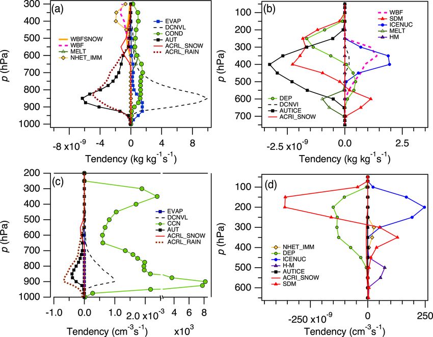
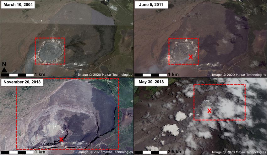
7756        K. H. Breen et al.: Effect of volcanic emissions on clouds during the 2008 and 2018 Kilauea degassing events

Figure 2. AOD anomalies (from left) for MODIS observations and for GEOS simulations using actual emissions (2008_1× and 2018_1×)
calculated against GEOSCLIM and the zero-emissions scenarios (2008_0× and 2018_0×) during JJA 2008 (top panels) and MJJ 2018
(bottom panels). The rightmost column shows normalized zonal mean anomalies for MODIS (blue) and GEOS against GEOSCLIM (green)
and zero emissions (black).

Figure 3. Like Fig. 2 but showing CF anomalies during JJA 2008 (top panels) and MJJ 2018 (bottom panels).

ural variability. Satellite retrievals are also influenced by em-    for supersaturation but MERRA-2 does not, and T is less
pirical definitions of cloudy and non-cloudy regions, adding         constrained by observations (Gelaro et al., 2017). The dis-
uncertainty (Pincus et al., 2012). Given this, it is remarkable      crepancy may also be exacerbated by artifacts in the retrieval.
that the CF anomaly against the climatology is in relatively         GOCCP tends to underestimate the presence of thin cirrus
good agreement with the satellite retrieval, demonstrating the       clouds and may overestimate low-level clouds in the pres-
skill of GEOS in reproducing clouds during volcanic events.          ence of high aerosol loading (Chepfer et al., 2010). GEOS
   To examine the cloud vertical structure during the two de-        was, however, able to simulate an anomalous increase in CF
gassing events, GEOS results for the 2008_1× and 2018_1×             above 800 hPa between 20 and 25◦ N in 2008 as seen in the
simulations were compared against CALIPSO-GOCCP, as                  retrieval. Similarly, there was a strong increase in CF in 2018
shown in Figs. 4 and 5, respectively. During both events, pre-       across the domain, although GEOS predicted a much larger
dominant cloud layers were found at 900 and 200 hPa, corre-          anomaly effect on cirrus clouds. Again, the discrepancy may
sponding to low-level trade cumulus and in situ formation of         be the result of a lack of sensitivity to thin cirrus clouds
thin cirrus clouds, respectively. The cloud vertical structure       in GOCCP.
during both events was similar, indicating a strong meteoro-            Another interesting feature of Figs. 4 and 5 is the presence
logical control. This was well-captured by the GEOS simula-          of mid-level altocumulus clouds, likely maintaining some
tions; the model, however, tended to overestimate high-level         supercooled water. In GOCCP, the SCF (i.e., the fraction
clouds and underestimate low-level clouds, particularly dur-         of condensate remaining as liquid at T < 273 K) decreased
ing the 2018 event (Fig. 5). This may result from replaying          sharply at around 550 hPa in both years but surprisingly re-
temperature to the reanalysis (Sect. 3.2) but letting water va-      mained significant (> 0.1) up to 200 hPa where homoge-
por evolve freely during the simulations. Such a configura-          neous ice nucleation glaciated the remaining water. This was
tion tends to overestimate relative humidity, particularly at        particularly true in 2018 when GOCCP showed enhanced
cirrus levels, because the two-moment microphysics allows            SCF relative to the climatology. GEOS showed similar be-

Atmos. Chem. Phys., 21, 7749–7771, 2021                                                https://doi.org/10.5194/acp-21-7749-2021
K. H. Breen et al.: Effect of volcanic emissions on clouds during the 2008 and 2018 Kilauea degassing events               7757

Figure 4. Zonal mean anomalies for JJA supercooled cloud fraction (1SCF) and cloud fraction (1CF) from the GEOS (top panels) sim-
ulation and the CALIPSO-GOCCP (bottom panels) dataset. Also shown are the anomalies with respect to the 2007–2017 climatology
(excluding 2008).

Figure 5. Like Fig. 4 but for MJJ 2018.

havior whereby the supercooled layer (0 < SCF < 1) was             suggest a deepening of clouds in the presence of aerosol and
deeper in 2018 than in 2008, particularly near the summit          is analyzed in Sect. 4.4
crater (≈ 25◦ N). The supercooled layer was almost 100 hPa
higher in GEOS than in GOCCP, indicating differences in ice        4.1   Liquid clouds
and liquid partitioning between the model and the retrieval;
this may be explained by the different definitions of SCF
                                                                   Figures 6 and 7 show anomalies in Reff , CDNC, COD, and
in each case. In GEOS, SCF is calculated on a mass basis,
                                                                   LWP for MODIS and the GEOS control simulations (Ta-
whereas in GOCCP it corresponds to the frequency of pixels
                                                                   ble 2) during the 2008 and 2018 degassing events, respec-
that are classified as ice. The positive anomaly in SCF may
                                                                   tively. Domain mean anomalies are summarized in Table 3.

https://doi.org/10.5194/acp-21-7749-2021                                           Atmos. Chem. Phys., 21, 7749–7771, 2021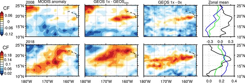
7758        K. H. Breen et al.: Effect of volcanic emissions on clouds during the 2008 and 2018 Kilauea degassing events

Figure 6. Anomaly in liquid cloud properties during JJA 2008 for (from top) Reff (µm, shown as ER), COD, CDNC (m−3 ), and LWP (g m−2 ).
Anomalies are shown (from left) for MODIS observations and for GEOS simulations calculated against GEOSCLIM and the zero-emissions
scenario. The rightmost column shows normalized zonal mean anomalies for MODIS (blue) and GEOS against GEOSCLIM (green) and zero
emissions (black).

Figure 7. Like Fig. 6 but for MJJ 2018.

Atmos. Chem. Phys., 21, 7749–7771, 2021                                                 https://doi.org/10.5194/acp-21-7749-2021
K. H. Breen et al.: Effect of volcanic emissions on clouds during the 2008 and 2018 Kilauea degassing events 7759
Table 3. Anomalies for liquid cloud properties, AOD, and CF. Values in parentheses are the p values associated with a one-sided Student’s t
test against the long-term mean.
Experiment Exp vs. climatology (excluding 2008) Exp vs. 0×
Reff COD CDNC LWP TWP AOD CF Reff COD CDNC LWP TWP AOD CF
(µm) (–) (m−3 ) (g m2 ) (g m2 ) (–) (–) (µm) (–) (m−3 ) (g m2 ) (g m2 ) (–) (–)
−0.58 4.63 16.04 8.77 8.31 0.01 −0.03 −0.65 3.77 15.68 6.82 7.17 0.03 0.02
2008_1×
(0.08) (0.12) (0.23) (0.19) (0.15) (0.40) (0.41) (0.07) (0.17) (0.24) (0.27) (0.19) (0.07) (0.63)
−1.31 10.70 40.06 18.99 19.34 0.07 −0.01 −1.37 9.84 39.71 17.04 18.21 0.09 0.03
2008_5×
(0.01) (0.02) (0.01) (0.05) (0.02) (0.07) (0.78) (0.01) (0.02) (0.01) (0.06) (0.02) (0.04) (0.32)
−0.58 4.63 16.04 8.77 8.70 0.01 −0.03 −0.45 2.31 13.55 4.03 4.90 0.02 0.01
2008_PH2km
(0.08) (0.12) (0.23) (0.19) (0.13) (0.40) (0.41) (0.07) (0.17) (0.24) (0.27) (0.17) (0.07) (0.63)
−0.75 0.46 21.53 0.65 −0.89 0.03 −0.02 – – – – – – –
MODIS (2008)
(0.26) (0.18) (1.00) (0.52) (0.74) (0.04) (0.50) (–) (–) (–) (–) (–) (–) (–)
−1.06 7.69 26.65 15.30 45.71 0.10 0.15 −1.23 8.30 28.61 10.07 18.09 0.10 0.02
2018_1×
(0.15) (0.13) (0.10) (0.08) (0.07) (0.16) (0.18) (0.11) (0.12) (0.08) (0.16) (0.28) (0.15) (0.78)
−0.60 0.69 19.43 5.09 25.81 0.11 0.13 – – – – – – –
MODIS (2018)
(0.14) (0.24) (0.02) (0.21) (0.23) (0.00) (0.20) (–) (–) (–) (–) (–) (–) (–)
Table 4. R 2 values for the comparison of GEOS normalized zonal anomalies for liquid clouds against MODIS.
Experiment MODIS anomaly vs. GEOS 1×-clim MODIS anomaly vs. GEOS 1×-0×
Reff COD CDNC LWP TWP AOD CF Reff COD CDNC LWP TWP AOD CF
(µm) (–) (m−3 ) (g m2 ) (g m2 ) (–) (–) (µm) (–) (m−3 ) (g m2 ) (g m2 ) (–) (–)
2008_1× 0.49 0.70 0.30 0.57 0.68 0.66 0.68 0.45 0.45 0.40 0.26 0.02 0.88 0.01
2008_PH2km 0.49 0.70 0.30 0.57 0.65 0.66 0.68 0.45 0.45 0.40 0.26 0.01 0.88 0.01
2018_1× 0.01 0.31 0.67 0.58 0.24 0.91 0.13 0.23 0.33 0.83 0.41 0.22 0.86 0.28
Table 4 shows the coefficient of determination (R 2 ) between however, well-correlated (R 2 > 0.5) for CDNC and AOD
the MODIS and the GEOS normalized zonal mean anoma- (Table 4). The discrepancies in LWP and COD absolute
lies. During both the 2008 and the 2018 events, GEOS was anomalies were likely due to variation in SSTs inside the do-
able to capture the geographical distribution of the anoma- main and the lack of a cloud albedo–SST feedback in our
lies apparent in the MODIS retrievals for liquid clouds. simulations.
Student’s t tests indicated that the anomalies were statisti- SO2 emissions at the Mauna Loa Observatory (19.5◦ N,
cally significant, typically to a 70 %–80 % level (p < 0.3, 155.6◦ W) peaked in JJA 2008 relative to the 1995–2008 sea-
except for AOD and CF in 2008, which were significant sonal mean, with prevailing La Niña conditions (Potter et al.,
only to 60 %) for Reff and CDNC more so than for other 2013). Thus, it is likely that the degassing event contributed
variables (Table 3). For the 2008_1× experiment, the mag- to lower SSTs, hence lowering surface evaporation rates and
nitude of the Reff and CDNC domain-averaged anoma- LWP. The negative anomaly in LWP in the southernmost
lies (−0.58 µm and 16.04 cm−3 , respectively) was in close part of the domain evident in 2008 is also missing in the
agreement with MODIS (−0.75 µm and 21.53 cm−3 , respec- 2018 event due to neutral ENSO conditions in the latter
tively) and well-correlated with the satellite retrievals (Ta- (NOAA, 2020), indicating that ENSO exerted a strong me-
ble 4). These values are also close to the anomalies calcu- teorological control that could have drowned out ACI signa-
lated against the 2008_0× simulation, suggesting a micro- tures in the former. Another reason behind the larger aerosol
physical control on Reff and CDNC. On the other hand, al- effects on COD and LWP simulated by GEOS than ob-
though the COD and LWP normalized anomalies are well- served by MODIS may lie in differences in phase partitioning
correlated between GEOS and MODIS, the model overes- (i.e., liquid vs. ice) (Marchant et al., 2016). To help identify
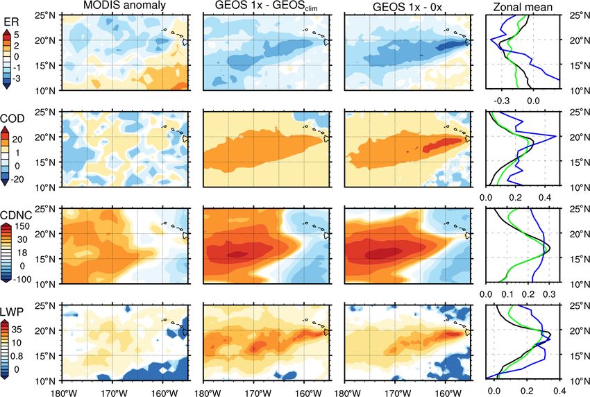
timated their absolute value. Similarly, in 2018 the GEOS thin cirrus clouds, measured top-of-the-atmosphere (TOA)
and MODIS anomalies in Reff (−1.06 µm vs. −0.60 µm) and reflectance at 1.38 µm is used to partition high-altitude cir-
CDNC (26.65 cm−3 vs. 19.43 cm−3 ) were in better agree- rus clouds from underlying liquid clouds. This method is
ment than for COD (7.69 vs. 0.69) and LWP (15.30 g m−2 strongly influenced by the relative humidity of the atmo-
vs. 5.09 g m−2 ). Normalized zonal mean anomalies were, spheric column. Therefore, areas with low column water va-
https://doi.org/10.5194/acp-21-7749-2021 Atmos. Chem. Phys., 21, 7749–7771, 20217760 K. H. Breen et al.: Effect of volcanic emissions on clouds during the 2008 and 2018 Kilauea degassing events
por amount may have more clouds partitioned to the ice well as the efficiency with which the new particles can pro-
phase than is realistic. This is important because 2008 was mote ice crystal formation (Barahona et al., 2010). Addition-
a La Niña year, and the relative humidity in the atmospheric ally, the presence of aerosols in the upper troposphere was
column was below climatological values, so LWP anoma- not apparent in a Gaussian-like plume emanating from the
lies may appear low due to enhanced partitioning to the ice Kilauea volcano, as was the case for liquid clouds; therefore,
phase in the MODIS cloud-phase classification algorithm. the identification of ACIs for ice clouds was less straightfor-
Even in 2018, most of the total water path (TWP) anomaly ward.
resulted from an increase in the ice water path, indicating Figure 8 shows that during the 2008 event, the aerosol
strong partitioning to the ice phase in the MODIS retrieval plume did not significantly alter the properties of ice clouds.
(Table 4). The 2008_1×–GEOSCLIM anomalies in ice clouds appeared
Overall, more robust correlations (R 2 > 0.5) resulted spatially consistent with MODIS anomalies for COD and
when the anomalies were calculated against the GEOSCLIM IWP, whereas 2008_1×–0× showed little to no variability in
than against the no-emissions scenarios (Table 4). This in- the domain. As shown in Table 6, there was high correlation
dicated that while both GEOS climatology and 0× cases between MODIS and the 2008_1×–GEOSCLIM normalized
included aerosol loading consistent with MODIS retrievals zonal mean anomalies for COD (R 2 = 0.84) and IWP (R 2 =
(Fig. 2, Table 4), correlations with observed data for liquid 0.93). These correlations substantially decreased when con-
clouds were sensitive to meteorological effects captured by sidering comparisons between MODIS and the 2008_1×–
the MODIS and GEOS climatologies. MODIS TWP anoma- 2008_0× difference. For COD in 2008, the latter seemed to
lies (for which TWP is the sum of LWP and IWP) in 2018 retain some correlation (R 2 = 0.29) and may indicate some
were about 20× higher than those reported for the 2008 event level of microphysical control on the observed anomalies.
(Table 3), suggesting that ACIs for 2018 were not limited to This suggested that most of the observed ice cloud anomaly
liquid clouds. in 2008 resulted from meteorological and SST variability.
We found that effects on liquid clouds were more sta- Prevailing La Niña conditions in 2008 likely reduced relative
tistically significant in 2018 than in 2008 for both ob- humidity within the atmospheric column, particularly in the
served (MODIS) and simulated (GEOS) cloud properties. upper troposphere, thereby limiting the supply of water vapor
In 2018, the magnitude and significance level of the simu- necessary for ice crystal nucleation and growth. Anomalous
lated anomalies against GEOSCLIM were close to those cal- conditions in ice clouds with respect to climatological and
culated against 2018_0×, indicating that increased aerosol background conditions, however, were not statistically sig-
loading, regardless of injection height, resulted in the height- nificant (Table 5).
ened development of liquid cloud droplets and that these ef- Similar to the 2008 event, there seemed to be a strong me-
fects could be attributed to volcanic degassing as opposed teorological component during MJJ 2018 degassing because
to regional meteorology. The results of the 2008_5× run the spatial correlation of the 2018_1×–GEOSCLIM results
were in general highly statistically significant (p < 0.05) appeared consistent with MODIS anomalies (Fig. 9). Addi-
and agreed in magnitude with the 2018_1× experiment. tionally, correlations between MODIS and GEOSCLIM zonal
The similarities in the magnitudes of simulated anomalies mean anomalies were higher (R 2 ≥ 0.2) than for the MODIS
for 2008_5× and 2018_1× suggested that increased aerosol vs. 2018_1×–2018_0× correlations, with the exception of
loadings would have been sufficient to overcome meteoro- IWP (R 2 = 0.32) (Table 6). Unlike the 2008 event, the
logical effects, which dampened the 2008 JJA anomalies with 2018_1×–2018_0× anomalies showed variability within the
respect to long-term behavior. This and the similarities in domain that was of similar magnitude to and appeared spa-
spatial patterns (i.e., anomalies largely constrained by and tially consistent with GEOSCLIM anomalies (Fig. 9), indicat-
maximized within the plume domain) for cloud anomalies in ing that not all ACIs in ice clouds could be attributed to mete-
JJA 2008 (Fig. 6) and MJJ 2018 (Fig. 7) suggested a thresh- orology alone. Figure 9 shows similar spatial distributions for
old response to overcome meteorological effects that was observed and simulated anomalies within the plume domain,
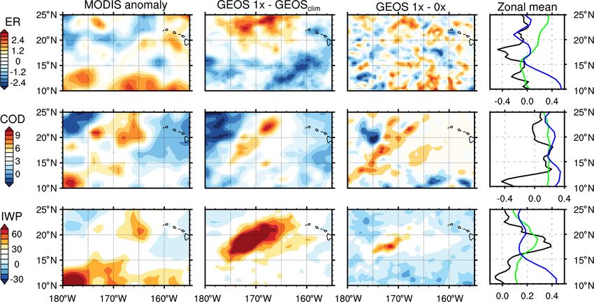
largely controlled by emissions. in particular between 175 and 165◦ W. Whereas for Reff
and COD anomalous cloud properties appeared to be re-
4.2 Ice clouds lated to meteorological variability, IWP anomalies appeared
to have a strong microphysical component. The MODIS and
The volcanic plume height during peak degassing periods GEOSCLIM anomalies for IWP in 2018 were of the same
varied significantly between 2008 and 2018; therefore, we order of magnitude at 20.59 and 30.41 g m−2 , respectively
expected the strength of ACIs for ice clouds to be partially (Table 5), whereas the GEOS IWP 2018_1×–2018_0× dif-
dependent on the availability of INPs. It is likely that the ference was ≈ 8.03 g m−2 . Although the strength of the ob-
plume introduced SO2 and ash particles to the upper tropo- served effect was better represented by the GEOSCLIM IWP
sphere – directly in 2018 and via convection in 2008. The anomaly, the IWP correlation for MODIS vs. 2018_1×–
effects of INPs on ice cloud development strongly depend on 2018_0× was slightly higher than against the climatol-
the microphysical processes dominating cloud evolution as ogy (R 2 = 0.32 vs. R 2 = 0.23); we found this difference to
Atmos. Chem. Phys., 21, 7749–7771, 2021 https://doi.org/10.5194/acp-21-7749-2021K. H. Breen et al.: Effect of volcanic emissions on clouds during the 2008 and 2018 Kilauea degassing events 7761
Figure 8. Ice cloud anomalies during JJA 2008 for (from top) Reff (µm, shown as ER), COD (–), and IWP (g m2 ). Anomalies are shown
(from left) for MODIS observations and for GEOS simulations calculated against GEOSCLIM and the zero-emissions scenario. The rightmost
column shows normalized zonal mean anomalies for MODIS (blue) and GEOS against GEOSCLIM (green) and zero emissions (black).
Figure 9. Like Fig. 8 but for MJJ 2018.
be significant at the 95 % confidence level. This strongly some of the anomalies, particularly for ice clouds (Ta-
suggested a significant microphysical control on the IWP ble 5) and for the 2018 event, although the effect was
anomaly during the 2018 event. small. Similarities between MODIS and GEOS results for
the 2008_5× and 2018_1× experiments on liquid clouds
4.3 Role of injection height and ash content (Table 3) indicated that increased aerosol loadings during
the 2008 event mimicked effects on liquid cloud formation
Domain-averaged CDNC varied widely between the differ- during the 2018 event, most notably for CDNC and AOD.
ent experiments except for the cases with elevated plume This showed that liquid cloud sensitivity to the first AIE
heights (2008_PH2km and 2018_PH4km), which essen- was dominated by aerosol loadings as opposed to plume
tially overlapped with the 2008_1× and 2018_1× exper- morphology during the 2008 event. Increasing plume height
iments, respectively (Figs. 10 and 11). Despite this, in- in concert with aerosol loadings exceeding 20 kt SO2 d−1
creasing the plume height yielded sizable differences in (2018_PH4km) reduced the anomaly in IWP and COD
https://doi.org/10.5194/acp-21-7749-2021 Atmos. Chem. Phys., 21, 7749–7771, 20217762 K. H. Breen et al.: Effect of volcanic emissions on clouds during the 2008 and 2018 Kilauea degassing events
Figure 10. Zonal mean vertical profiles for cloud fraction (CF), liquid (Qliq ) and ice (Qice ) mixing ratios, total detrained condensate tendency
(CNV_DQLDT), cloud droplet (CDNC), and ice crystal (ICNC) number concentration for the 2008 JJA season. Notice that MERRA-2 and
GOCCP data are included for CF only.
Figure 11. Equivalent to Fig. 10 but for the 2018 MJJ season.
by less than 5 % relative to the 2018_1× experiment (Ta- 4.4 Microphysical controls on ACIs
ble 6). Similarly, accounting for ash INP (2018_PH4km_ash)
slightly increased the COD and IWP anomalies (Table 5), al- Figures 10 and 11 summarize the experiments performed in
though it had opposite effects on the ice crystal mixing ratio, this work. Also shown are the CF values from MERRA-2 and
Qice , and ICNC, with the former lower and the latter higher GOCCP. In all runs and for both events, the vertical profile
than in the 2018_PH4km experiment (Fig. 5). This is fur- of CF was remarkably similar, with two predominant cloud
ther analyzed in Sect. 4.4. The correlations between GEOS layers associated with shallow cumulus and warm cirrus–
anomalies and MODIS for Reff and COD in ice clouds im- altocumulus. This vertical structure was in agreement with
proved slightly with the inclusion of ash INP (Table 6). GOCCP data (also shown in Figs. 4 and 5). Compared to
GOCCP, GEOS tended to overestimate high-level CF and un-
Atmos. Chem. Phys., 21, 7749–7771, 2021 https://doi.org/10.5194/acp-21-7749-2021K. H. Breen et al.: Effect of volcanic emissions on clouds during the 2008 and 2018 Kilauea degassing events 7763
Table 5. Anomalies for ice cloud properties. Values in parentheses are the p values associated with a one-sided Student’s t test against the
long-term mean.
Experiment Exp vs. climatology Exp vs. 0×
Reff COD IWP Reff COD IWP
(µm) (–) (g m2 ) (µm) (–) (g m2 )
0.25 −0.13 −0.46 −0.04 0.00 0.35
2008_1×
(0.73) (0.19) (0.80) (0.96) (0.99) (0.85)
0.53 0.79 −1.46 – – –
MODIS (2008)
(0.60) (0.40) (0.55) (–) (–) (–)
0.95 0.58 30.41 −0.09 0.04 8.03
2018_1×
(0.39) (0.21) (0.16) (0.92) (0.91) (0.63)
1.12 0.58 30.38 0.08 0.04 8.00
2018_PH4km
(0.32) (0.20) (0.16) (0.94) (0.90) (0.62)
−4.33 0.63 36.44 −5.38 0.10 14.06
2018_PH4km_ash
(0.01) (0.18) (0.15) (0.01) (0.79) (0.47)
0.00 3.03 20.59 – – –
MODIS (2018)
(0.27) (0.18) (0.26) (–) (–) (–)
Table 6. R 2 values comparing GEOS normalized zonal anomalies averaged rates of different cloud microphysical processes
for ice clouds against MODIS. that took place during each event. They are distinguished
by processes that affect the mass and number concentra-
Experiment MODIS anomaly vs. MODIS anomaly vs. tion of liquid droplets and ice crystals. Both events showed
GEOS 1×-clim GEOS 1× vs. 0× similar features regarding processes affecting liquid conden-
Reff COD IWP Reff COD IWP sate and CDNC (Figs. 12a, c and 13a, c). As expected, liq-
(µm) (–) (g m2 ) µm) (–) (g m2 ) uid cloud microphysics were dominated by CCN activation
2008_1× 0.25 0.84 0.93 0.01 0.29 0.04 and condensation (i.e., by droplet formation on sulfate parti-
2018_1× 0.23 0.15 0.23 0.03 0.16 0.32 cles). Cumulus detrainment (DCNVL) is a significant source
2018_PH4km 0.25 0.16 0.20 0.14 0.04 0.34
2018_PH4km_ash 0.27 0.39 0.15 0.29 0.01 0.21 of condensate but only plays a minor role in determining
CDNC. The main sinks of liquid mass and number concen-
tration are droplet autoconversion (AUT) and accretion of
cloud droplets by rain (ACRL_RAIN). The CCN source rate
derestimate it near the surface. This is discussed in Sect. 4;
in 2018 (Fig. 13c) was about 3 times that of 2008 (Fig. 12);
however, here we also note that there is a high uncertainty
however, the liquid condensate tendencies shown in panel (a)
in the retrieval during these periods. For example, GEOS-
in both figures were of the same magnitude. Thus, the mech-
simulated high-level clouds were in better agreement with
anism for the decrease in Reff was an increase in CCN acti-
MERRA-2, whereas low-level CF in the latter was much
vation and hence CDNC, which did not translate into a pro-
lower than indicated by GOCCP. Examination of the GEOS
portional increase in liquid mass (i.e., the first AIE). This is
simulations suggested that CF around 800 hPa was slightly
revealed in Figs. 10 and 11 as large increases in CDNC, but
higher for high aerosol loading than for the no-emissions ex-
only slight increases in Qliq , between the 1× and 0× experi-
periments, indicating deepening of clouds from the injection
ments.
of aerosol. This was supported by an increase in Qliq be-
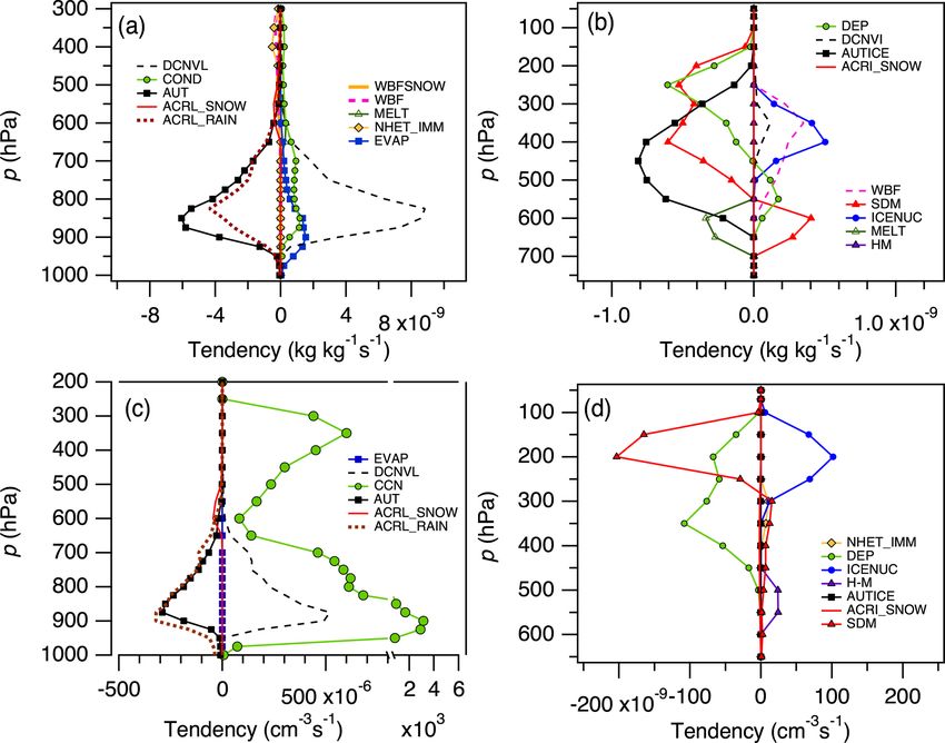
It is not clear why the liquid autoconversion tenden-
tween the 1× and the 0× experiments and runs along an
cies (AUTs) were almost insensitive to the aerosol load. Most
enhanced detrained mass tendency, CNV_DQLDT, indicat-
likely, the liquid mass and number concentration sinks were
ing predominant convective effects. In general, the GEOS
controlled by accretion rather than autoconversion. This is
climatology (CLIM) tended to show lower values of liquid
depicted in Fig. 14. Figure 14a and c show that the autocon-
and ice properties than the 0× experiments, with the notable
version sinks for mass and number were similar across all
exception of the ice mixing ratio and number concentration
simulation experiments, even those without volcanic emis-
in 2008.
sions (i.e., 2008_0× and 2018_0×), despite CCN activation
These effects can be understood in light of the modi-
tendencies varying by a factor of 4. Our results indicated
fication to dominant microphysical tendencies by elevated
that ACRL_RAIN was, however, enhanced for GEOS ex-
aerosol emissions. Figures 12 and 13 show the seasonally
https://doi.org/10.5194/acp-21-7749-2021 Atmos. Chem. Phys., 21, 7749–7771, 2021You can also read