Geometric estimation of volcanic eruption column height from GOES-R near-limb imagery - Part 1: Methodology - Recent
←
→
Page content transcription
If your browser does not render page correctly, please read the page content below
Atmos. Chem. Phys., 21, 12189–12206, 2021
https://doi.org/10.5194/acp-21-12189-2021
© Author(s) 2021. This work is distributed under
the Creative Commons Attribution 4.0 License.

Geometric estimation of volcanic eruption column height from
GOES-R near-limb imagery – Part 1: Methodology
Ákos Horváth1 , James L. Carr2 , Olga A. Girina3 , Dong L. Wu4 , Alexey A. Bril5 , Alexey A. Mazurov5 ,
Dmitry V. Melnikov3 , Gholam Ali Hoshyaripour6 , and Stefan A. Buehler1
1 Meteorological   Institute, Universität Hamburg, Hamburg, Germany
2 Carr  Astronautics, Greenbelt, MD, USA
3 Institute of Volcanology and Seismology, Far East Branch of the Russian Academy of Sciences (IVS FEB RAS),

Petropavlovsk-Kamchatsky, Russia
4 NASA Goddard Space Flight Center, Greenbelt, MD, USA
5 Space Research Institute of the Russian Academy of Sciences (SRI RAS), Moscow, Russia
6 Institute of Meteorology and Climate Research, Karlsruhe Institute of Technology (KIT), Karlsruhe, Germany

Correspondence: Ákos Horváth (akos.horvath@uni-hamburg.de, hfakos@gmail.com)

Received: 21 February 2021 – Discussion started: 23 March 2021
Revised: 2 July 2021 – Accepted: 6 July 2021 – Published: 16 August 2021

Abstract. A geometric technique is introduced to estimate        atmospheric dispersion models, which require the eruptive
the height of volcanic eruption columns using the gener-         source parameters, especially plume height and the mass
ally discarded near-limb portion of geostationary imagery.       eruption rate (MER), as key inputs (Peterson et al., 2015).
Such oblique observations facilitate a height-by-angle esti-     Plume height and MER are related by dynamics, and the lat-
mation method by offering close-to-orthogonal side views         ter scales approximately as the fourth power of the former.
of eruption columns protruding from the Earth ellipsoid.         Thus, a small error in plume height leads to a large error
Coverage is restricted to daytime point estimates in the im-     in MER, estimates of which can consequently have a fac-
mediate vicinity of the vent, which nevertheless can pro-        tor of 10 uncertainty (Bonadonna et al., 2015). The mass
vide complementary constraints on source conditions for the      eruption rate is commonly estimated from plume height ob-
modeling of near-field plume evolution. The technique is         servations using semiempirical relationships, Sparks–Mastin
best suited to strong eruption columns with minimal tilt-        curves, derived from buoyant plume theory and historical
ing in the radial direction. For weak eruptions with severely    eruption data (Mastin et al., 2009; Sparks et al., 1997). An
bent plumes or eruptions with expanded umbrella clouds           alternative is to use simplified 1D cross-section-averaged
the radial tilt/expansion has to be corrected for either visu-   (Folch et al., 2016) or 2D Gaussian (Volentik et al., 2010)
ally or using ancillary wind profiles. Validation on a large     plume rise models, which can be inverted efficiently to esti-
set of mountain peaks indicates a typical height uncertainty     mate MER from plume height.
of ±500 m for near-vertical eruption columns, which com-            Many techniques have been developed over the years to
pares favorably with the accuracy of the common tempera-         measure volcanic plume height (for a comparative overview
ture method.                                                     see Dean and Dehn, 2015; Merucci et al., 2016; Zakšek et al.,
                                                                 2013; and references therein). Ground-based methods rely on
                                                                 weather radars, lidars, or video surveillance cameras. Space-
                                                                 based methods include radar and lidar observations, radio oc-
1   Introduction                                                 cultation, backward trajectory modeling, geometric estimates
                                                                 from shadow length and stereoscopy, and radiometric esti-
Volcanic eruptions pose significant hazards to aviation, pub-    mates utilizing the CO2 and O2 absorption bands and infrared
lic health, and the environment (Martí and Ernst, 2005). Risk    (IR) channels.
assessment and mitigation of these hazards is supported by

Published by Copernicus Publications on behalf of the European Geosciences Union.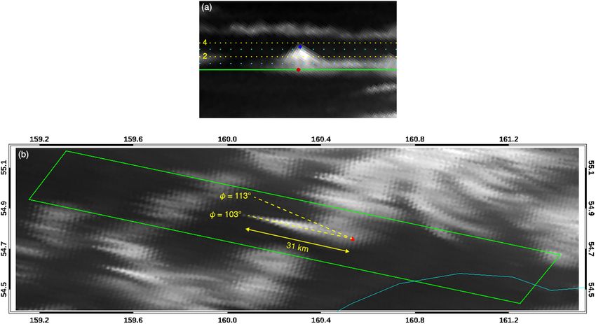
12190                                  Á. Horváth et al.: Geometric estimation of volcanic eruption column height – Part 1

   The height retrieval technique offering the best spatial        plumes compared to lidar or stereo heights generally consid-
and temporal coverage globally is the spaceborne “temper-          ered the most accurate (Flower and Kahn, 2017; Pavolonis et
ature method”, which is based on IR brightness temperatures        al., 2013; Thomas and Siddans, 2019).
(BTs) routinely available from a large suite of imaging ra-           Globally applicable near-real-time techniques, such as
diometers aboard both polar orbiter and geostationary satel-       the satellite temperature method, are nevertheless indispens-
lites. In its simplest and still oft used single-channel form,     able to support operations at volcanic ash advisory cen-
the method determines plume height by matching the 11 µm           ters and mitigate aviation and health hazards. The single-
BT to a temperature profile obtained from a radiosounding or       channel temperature method is part of the VolSatView infor-
a numerical forecast, assuming an opaque plume in thermal          mation system (Bril et al., 2019; Girina et al., 2018; Gordeev
equilibrium with its environment. Both of these assumptions,       et al. 2016) operated by the Kamchatka Volcanic Erup-
however, can be invalid.                                           tion Response Team (KVERT; Girina and Gordeev, 2007).
   The plume tops of the largest explosions, especially ones       The multichannel retrievals form the core of the VOLcanic
that penetrate the stratosphere, might be in thermal disequi-      Cloud Analysis Toolkit (VOLCAT) and are produced from
librium due to decompression cooling in a stably stratified        Geostationary Operational Environmental Satellite-R Series
atmosphere. Undercooling can lead to a cloud top that is tens      (GOES-R) and Himawari-8 imager data by the National
of degrees colder than the minimum temperature of the sur-         Oceanic and Atmospheric Administration (NOAA) and the
rounding ambient, in which case the satellite-measured BT          Japanese Meteorological Agency (JMA). The pursuit of new
cannot be converted to height (Woods and Self, 1992). Ther-        techniques is still worthwhile though, given the large uncer-
mal disequilibrium of the opposite sign might also occur be-       tainty of existing retrieval algorithms (von Savigny et al.,
cause the increased absorption of solar and thermal radiation      2020).
by volcanic ash can cause significant local heating (Muser et         Our proof-of-concept study introduces a simple geomet-
al., 2020), resulting in negatively biased height retrievals.      ric technique to derive point estimates of eruption column
   A more common problem is that the plume, especially its         height in the vicinity of the vent from side views of the plume
dispersed part further from the vent, is semitransparent to        captured in near-limb geostationary images. In planetary sci-
IR radiation and deviates strongly from blackbody behavior;        ence, topography is often estimated by the radial residuals
hence, the 11 µm BT is warmer than the effective radiative         to a best-fit ellipsoid along a limb profile. Such limb topog-
temperature. Surface contribution to the measured BT leads         raphy was derived for Io (Thomas et al., 1998), saturnian
to underestimated plume heights (Ekstrand et al., 2013). This      icy satellites (Nimmo et al., 2010; Thomas, 2010), and Mer-
low bias can be somewhat reduced by using only the mini-           cury (Oberst et al., 2011), to mention a few. Limb images
mum (dark pixel) BT of the plume least affected by surface         were also used to estimate the height of ice and dust clouds
radiation.                                                         on Mars (Hernández-Bernal et al., 2019; Sánchez-Lavega
   A more sophisticated treatment of semitransparency ef-          et al., 2015, 2018) and even the height of volcanic plumes
fects, however, requires BTs from multiple IR channels.            on Io (Geissler and McMillan, 2008; Spencer et al., 2007;
Pavolonis et al. (2013) developed a volcanic ash retrieval         Strom et al., 1979). Closer to home, near-limb images from
based on the 11 and 12 µm split-window channels and the            geostationary satellites were used to reconstruct the atmo-
13.3 µm CO2 absorption band, with the latter providing the         spheric trajectory of the 2013 Chelyabinsk meteor (Miller et
needed height sensitivity for optically thin mid- and high-        al., 2013) and study the altitude of polar mesospheric clouds
level plumes. The algorithm solves for the radiative tempera-      (Gadsden, 2000a, b, 2001; Proud, 2015; Tsuda et al., 2018).
ture, emissivity, and a microphysical parameter of the plume       Apart from these two applications, however, the near-limb
by optimal estimation. These parameters are then used to de-       portion of geostationary images is completely unused for any
termine plume height, effective ash particle radius, and mass      quantitative geophysical analysis.
loading for four different mineral types (andesite, rhyolite,         Here we exploit exactly these oblique observations, which
gypsum, and kaolinite) to account for uncertainty in chemi-        provide side views at almost a right angle of volcanic erup-
cal composition.                                                   tion columns protruding from the Earth ellipsoid. The pro-
   All brightness-temperature-based height retrievals are          posed height-by-angle technique is based on the finest-
however problematic near the tropopause due to the char-           resolution daytime visible channel images, and it is analo-
acteristic temperature inversion. Small lapse rates and            gous to the astronomical height retrievals and the height esti-
nonunique solutions lead to a significantly increased height       mation methods from calibrated ground-based video camera
uncertainty. Over- and underestimation are both possible           footage (Scollo et al., 2014). In particular, we take advan-
depending on whether the forecast temperature profile is           tage of the current best-in-class Advanced Baseline Imager
searched from top to bottom or bottom to top for a match-          (ABI) aboard the GOES-R satellites, which offers nominally
ing height. As a result of the listed error sources (emissivity,   500 m resolution red band imagery every 10 min combined
chemical composition, lapse rate), temperature methods have        with excellent georegistration (Schmit et al., 2017). The pa-
typical absolute uncertainties of 1–2 km for low- and mid-         per describes plume height estimation specifically from ABI
level (< 7 km) plumes and 3–4 km for high-level (> 7 km)           data, but the method is equally applicable to data from the

Atmos. Chem. Phys., 21, 12189–12206, 2021                                          https://doi.org/10.5194/acp-21-12189-2021
Á. Horváth et al.: Geometric estimation of volcanic eruption column height – Part 1                                                    12191

Figure 1. Horizontal (GIFOV, orange) and vertical (VIFOV, blue) spatial resolution of an ABI band 2 fixed grid pixel at the sub-satellite point
and the Sheveluch volcano in Kamchatka observed at a view zenith angle of θ ≈ 84◦ . The fixed grid has an angular resolution of 14 µrad in
both the east–west and the north–south directions and is rectified to the GRS80 ellipsoid as viewed from an idealized geostationary position.
Note the figure is not drawn to scale.

nearly identical Advanced Himawari Imager (AHI) aboard                    ther from GOES-17 than the sub-satellite point and observed
the Himawari third-generation satellites.                                 at VZA = 83.4◦ , leading to a VIFOV of ∼ 573 m. Thanks to
                                                                          this fine VIFOV, even small vertical features that would be
                                                                          sub-GIFOV were they oriented horizontally can in fact be
2     ABI and AHI limb observations                                       identified in near-limb images as they protrude from the el-
                                                                          lipsoid.
2.1    Full disk fixed grid image                                            The AHI angular sampling distance in the 0.64 µm visi-
                                                                          ble channel (band 3) is slightly smaller than 14 µrad, result-
We use the highest-resolution ABI 0.64 µm (band 2) level 1B               ing in a slightly larger 22 000 × 22 000-pixel full disk im-
radiances. The full disk view, which covers the entire Earth              age (Japan Meteorological Agency, HSD User’s Guide v1.3,
disk, is a 21 696 × 21 696-pixel image given on a fixed grid              2017). The AHI fixed grid is rectified to the World Geodetic
rectified to the Geodetic Reference System 1980 (GRS80)                   System 1984 (WGS84) reference ellipsoid, which is practi-
ellipsoid. The ABI fixed grid is an angle-by-angle coordi-                cally identical to the GRS80 ellipsoid for most applications
nate system that represents the vertical near-side perspective            (a tiny difference in flattening leads to a tiny difference in the
projection of the Earth disk from the vantage point of a satel-           polar radius). Another small difference is that the ABI full
lite in an idealized geosynchronous orbit 35 786 km above                 disk image applies a limb mask and excludes space pixels,
the Equator (GOES-R PUG L1B Vol 3 Rev 2.2, 2019). The                     while the AHI full disk image smoothly transitions into space
east–west and north–south fixed grid coordinates increase by              and does include space pixels; the latter is advantageous for
exactly 14 µrad per pixel in the final resampled image. This              the detection of eruptions very close to the limb.
14 µrad instantaneous field of view (IFOV) corresponds to                    The ABI data distributed by NOAA have excellent im-
a 500 m ground-projected instantaneous field of view (GI-                 age navigation and registration. The subpixel navigation er-
FOV or horizontal spatial resolution) at the equatorial sub-              rors are typically 1–2 µrad in both directions, with GOES-
satellite point observed with a view zenith angle (VZA) of                17 showing slightly larger errors than GOES-16 (Kalluri et
∼ 0◦ (satellite elevation angle ∼ 90◦ ), as sketched in Fig. 1.           al., 2018; Tan et al., 2019). It should be noted, however, that
At the near-limb locations of Kamchatka and the Kuril Is-                 ABI image navigation performance is at present evaluated
lands, however, the same IFOV corresponds to a GIFOV of                   mostly for scenes observed with VZA < 75◦ , in order to fil-
∼ 4 km, because these areas are observed at grazing angles                ter out low-quality measurements resulting from refraction
with VZA > 80◦ (satellite elevation angle < 10◦ ). The ∼ 8                effects and a large GIFOV. Georegistration quality near the
times larger pixel footprint near the limb renders images of              limb might therefore be poorer than the quoted values and
horizontal surface features very blurred.                                 will need further assessment.
   In contrast, the side of a vertically oriented object, such as            The geolocation accuracy of AHI aboard Himawari-8 is
a mountain peak or eruption column, is observed at a satel-               somewhat worse than that of ABI (Takenaka et al., 2020;
lite elevation angle (relative to the side) of almost 90◦ near            Yamamoto et al., 2020). The original AHI data provided by
the limb – the roles of zenith angle and elevation angle are re-          JMA are georegistered based on IR channels with a nominal
versed for vertical orientation. Thus, the local vertically pro-          resolution of 2 km. There is also a gridded AHI dataset by the
jected instantaneous field of view (VIFOV or vertical spa-                Center for Environmental Remote Sensing (CEReS) at Chiba
tial resolution) is only slightly coarser than the equatorial             University, which is more accurately georegistered based on
nadir GIFOV, because it scales linearly with distance to the              the visible channel with a nominal resolution of 500 m. In
satellite. For example, the Sheveluch volcano (also known                 this study, we used CEReS data V20190123, which can have
as Shiveluch) in northern Kamchatka is located ∼ 14 % fur-                navigation errors of about 1 pixel in band 3 images.

https://doi.org/10.5194/acp-21-12189-2021                                                 Atmos. Chem. Phys., 21, 12189–12206, 2021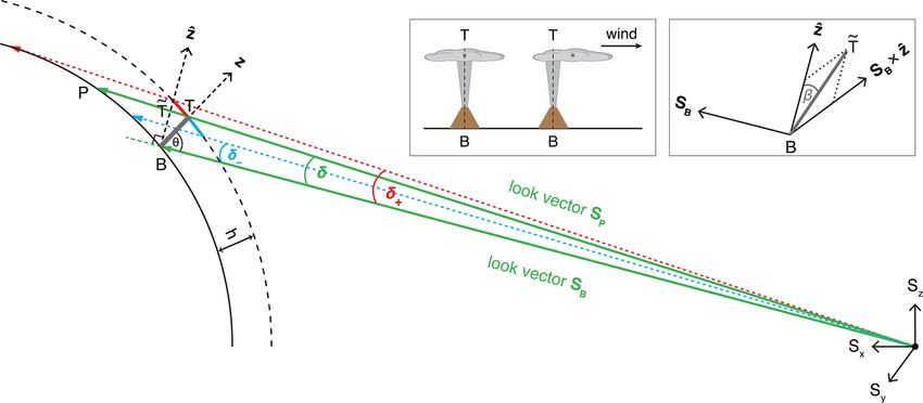
12192                                 Á. Horváth et al.: Geometric estimation of volcanic eruption column height – Part 1

Figure 2. Limb area between the 80◦ and 90◦ view zenith angle isolines of the GOES-16 (dotted magenta), GOES-17 (solid red), and
Himawari-8 (dashed blue) full disk. Triangles indicate volcanoes that erupted within the limb areas in the past 100 years.

   Note that a fixed grid image is in a map projection which      the volcanic eruption column and ash plume height. These
extremely distorts the shape and area of horizontal features      techniques will be used in Part 2 of the paper to validate
at the limb. For analyzing vertically oriented limb objects,      height estimates by the new method (Horváth et al., 2021).
however, it is the natural choice as it provides a fairly sharp      As an elementary model of a straight pillar of ash produced
side view with minimal foreshortening. Remapping the near-        by a strong eruption, consider a vertical column of height
limb portion of a fixed grid image into another projection        h with base B and top T protruding from the Earth ellip-
can give a considerably distorted view of vertical objects. For   soid, locally approximated by the tangent plane, as shown
example, the common equirectangular projection (also used         in Fig. 3a. We define a coordinate system with the origin
by NASA Worldview) introduces severe east–west stretch-           at B, x axis pointing north, and y axis pointing east. The
ing of higher-latitude mountains and eruption columns (see        sun-view geometry is described by the solar zenith and solar
Sect. 4).                                                         azimuth angles θ0 and φ0 and the satellite view zenith and
                                                                  view azimuth angles θ and φ (the azimuths correspond to
2.2    Limb volcanoes                                             the pixel-to-sun and pixel-to-sensor directions). The sensor-
                                                                  projected location of T in the satellite image is point P , the
We define an extended limb area in ABI and the very similar       shadow (or solar projection) of T is cast at point S, and the
AHI full disk images as the band of pixels with VZA > 80◦ .       vector from S to P is denoted D. The corresponding view
This criterion ensures that a near-vertical eruption column       and shadow geometry of a horizontally extended, dispersed
protruding from the Earth ellipsoid is observed at a close-       plume detached from the surface is illustrated in Fig. 3b, for
to-right angle. The limb areas for GOES-16, GOES-17, and          simplicity only for the case when the satellite is in the solar
Himawari-8 are shown in Fig. 2, which also plots the loca-        principal plane. Here the leading (farthest from the sun) edge
tion of volcanoes that erupted within these regions in the        of the plume can be taken as point T . The sun-view geom-
past 100 years. Historic eruption data were obtained from         etry angles, the sensor- and solar-projected locations of T ,
the Holocene Volcano List of the Global Volcanism Pro-            and the vector connecting them are known. But base point
gram (2013). The obliquely viewed volcanic subregions are         B, that is, the nadir-projected location of point T , is gener-
Iceland for GOES-16; the Kamchatka Peninsula, the Kuril           ally unknown. For the special case of a near-vertical column
Islands, the Mariana Islands, Papua New Guinea, southern          of ejecta, however, the base location can be approximated by
Chile, and the West Indies for GOES-17; and the Alaska            the surface (x,y) coordinates of the volcanic vent, which is
Peninsula, the southern Indian Ocean, and Antarctica for          available from geographical databases.
Himawari-8.

3     Geometric estimation of eruption column height              3.1   Method 1: height from sensor-projected length
      from one or two satellite views

Before describing the side view method in detail, we first        The above-ellipsoid height of column BT can be estimated
give a general overview of geometric techniques to retrieve       from its sensor-projected length in the x–y plane BP and the

Atmos. Chem. Phys., 21, 12189–12206, 2021                                         https://doi.org/10.5194/acp-21-12189-2021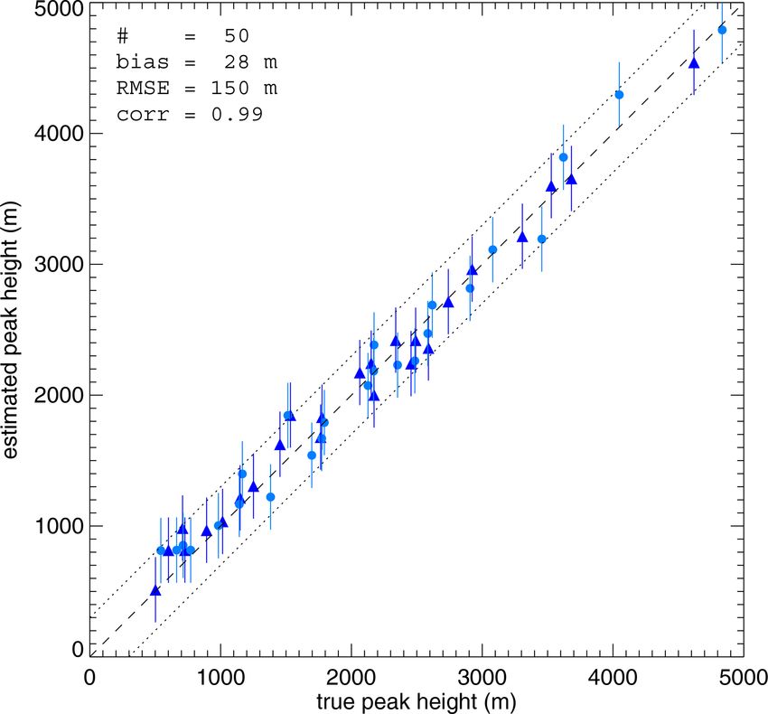
Á. Horváth et al.: Geometric estimation of volcanic eruption column height – Part 1                                                   12193

Figure 3. Sun-satellite-shadow geometry for (a) a narrow vertical eruption column under arbitrary viewing and illumination conditions and
(b) a horizontally expanded suspended ash layer in the solar principal plane of panel (a). In panel (b), the cyan line segment represents the
true (stick) shadow length, and the orange coloring indicates the area in the shadow of the ash layer.

view zenith angle θ simply as                                               The height estimate is formally less sensitive to errors in
                                                                         measured shadow length at large solar zenith angles around
      BP
h=         ,                                                (1)          sunrise or sunset. Determining the end of shadow location,
     tan θ                                                               however, can be particularly difficult at these times if the
assuming a flat Earth. Sensitivity to a given error in the               shadow falls near the day–night terminator. Another compli-
measured projected length decreases quickly with increas-                cation is that at certain sun-view geometries, the length of
ing view zenith angle. However, the GIFOV also increases                 the observed shadow differs from that of the true shadow –
rapidly at large θ . For example, a 1-pixel error in projected           “true” (stick) shadow length is defined by Eq. (2) as height
length at θ = 84◦ is ∼ 4 km, which translates to a height error          times the tangent of solar zenith angle. For the special case
of 420 m. In practice, it can be difficult to accurately deter-          of a narrow and tall vertical column, the potential difference
mine point P at very oblique view angles when using a tra-               between the observed and the true shadow lengths can only
ditional map projection due to potentially severe image dis-             be negative: when the sun and satellite are on the same side
tortions (e.g., east–west stretching in equirectangular projec-          of nadir (small relative azimuths), part of the true shadow
tion). For the highest plumes Earth’s curvature also has to be           might be obscured by the column itself. For most other sun-
accounted for.                                                           view geometries (medium-to-large relative azimuths), how-
                                                                         ever, the entire true shadow extending from the base of the
3.2    Method 2: height from true shadow length                          column is observed. In either case Eq. (2) can be used, be-
                                                                         cause the starting point of the shadow (the vent location)
In the same manner as described above, column height can                 is known, even when obscured, and, thus, the true shadow
also be estimated from the solar-projected column length                 length can be determined if the terminus of the shadow is
(i.e., true shadow) BS and the solar zenith angle θ0 as                  clearly observed.
       BS                                                                   For a horizontally extended ash layer detached from the
h=           .                                                  (2)      surface, on the other hand, the error in the observed shadow
      tan θ0
                                                                         length can be both negative and positive, and Eq. (2) is appli-
This method yields column height above the surface on                    cable to nadir satellite views only. The case of a suspended
which the shadow is cast. Equation (2) corresponds to the                ash layer under arbitrary viewing and illumination conditions
simplest case of a flat ocean or flat cloud surface; in the latter       is discussed in the next section.
case, the absolute height above the ellipsoid can be obtained
by adding the estimated cloud height. For shadows over land              3.3   Method 3: height from distance between plume
the calculations are more complex and require a digital ele-                   edge and shadow edge
vation model (DEM) to remove topography effects. A vol-
canic plume with a particularly bumpy top presents addi-                 The generalization of the stick shadow method to the more
tional difficulty, because the highest point (e.g., overshooting         common case of a horizontally expanded cloud or ash layer
top) might cast its shadow on the lower (and wider) parts of             was derived by Simpson et al. (2000a, b) and Prata and Grant
the plume rather than on the surface. In that case, the surface-         (2001). Here layer height is determined from the direction
measured shadow length leads to a height that underestimates             and length of vector D, which connects the terminus of the
the maximum plume height.                                                shadow (S) with the sensor-projected image location (P ) of

https://doi.org/10.5194/acp-21-12189-2021                                               Atmos. Chem. Phys., 21, 12189–12206, 2021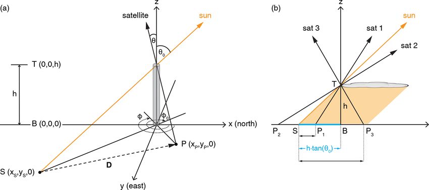
12194                                    Á. Horváth et al.: Geometric estimation of volcanic eruption column height – Part 1

the leading edge of the plume (T ). Vector D in this case is        the numerator being replaced by the apparent shadow length
the observed (apparent) shadow, whose length is generally           and tan θ0 in the denominator being replaced by a more com-
different from the true shadow length defined by Eq. (2), as        plicated formula, which depends on the view zenith and rel-
demonstrated in Fig. 3b for the principal plane. For example,       ative azimuth angles too.
if the satellite and the sun are on the same side of the nadir         Note that for a horizontal suspended ash layer only a single
line and θ < θ0 (satellite above the sun, sat 1 position), the      height estimate can be derived from the (edge) shadow using
observed shadow (P1 S) is foreshortened relative to the true        Eq. (8), which becomes Eq. (2) for nadir viewing. A vertical
shadow (BS), and if θ > θ0 (satellite below the sun, sat 2          column, however, represents a special case, for which two
position) no leading-edge shadow is observed due to obscu-          separate height estimates can be derived from the shadow,
ration by the plume. In contrast, if the satellite and the sun      using both Eqs. (2) and (8). This is so because for a column,
are on opposite sides of the nadir line (sat 3 position), the ap-   the surface projected location of top point T is known from
parent shadow (P3 S) is longer than the true shadow, because        three different directions: the satellite view (point P ), the so-
the satellite also observes the shadow cast under the leading       lar view (point S, the shadow terminus), and the effective
edge by other parts of the plume.                                   nadir view (base point B). The vector (parallax) between any
   For arbitrary viewing and illumination conditions, points        two of these surface projections can be used, in conjunction
P and S have the following horizontal coordinates on a flat         with the sun-view angles, to estimate the height: method 1 for
surface (Fig. 3a):                                                  BP (sensor projected length), method 2 for BS (true shadow
                                                                    length), and method 3 for P S (the apparent shadow, although
xP = h tan θ cos (φ − π )                                           this line segment is not in shadow for a column). For a sus-
yP = h tan θ sin (φ − π )                                           pended ash layer, however, the nadir-projected base point B
xS = h tan θ0 cos (φ0 − π )                                         is unknown, and thus only method 3 is applicable.
                                                                       In the practical implementation of Eq. (8), the satellite im-
yS = h tan θ0 sin (φ0 − π) .                                  (3)   age is first rotated so that one of its axes aligns with azimuth
Therefore, the components of vector D connecting S to P             φD and then the plume–shadow separation distance can be
are                                                                 easily calculated along an image row or column. The plume
                                                                    and shadow edges can be delineated visually by a human ob-
xD = hX                                                             server or more objectively by a wide variety of edge detection
yD = hY,                                                      (4)   algorithms (Canny, Roberts, Sobel, Prewitt, Laplacian, etc.).
                                                                    As before, a DEM is needed to remove topography effects
where                                                               when shadows over land are analyzed.

X = tan θ cos φ − tan θ0 cos φ0                                     3.4   Method 4: height from stereoscopy
Y = tan θ sin φ − tan θ0 sin φ0 .                             (5)
                                                                    The previous three methods estimate plume height from a
The direction (azimuth) and magnitude of D are respectively         single satellite image. This is possible in two special cases
                                                                  when an extra piece of information can be recovered from
               Y
φD = arctan                                             (6)         the image in addition to the sensor-projected plume top lo-
               X                                                    cation. One, for vertical eruption columns the location of the
and                                                                 base (i.e., the nadir-projected location of the top) can be ap-
       p                                                            proximated by that of the volcanic vent. Two, when shad-
|D| = h X 2 + Y 2 .                                           (7)   ows are visible they provide the projected location of a plume
                                                                    top/edge point from a second (the solar) perspective. There-
Direction φD is independent of h, as it is a function solely of     fore, these single-image methods can be considered as effec-
the sun-view geometry angles. Once the separation distance          tive “stereo” methods, because they use the surface locations
|D| between the plume edge and the shadow edge along az-            of a plume point projected from two different directions.
imuth φD is determined, the height of the plume edge can be            In the general case, column/plume height can be estimated
calculated from Eq. (7) as                                          by proper stereoscopy utilizing multiple views from at least
                                                                    two different directions (e.g., de Michele et al., 2019; Zakšek
         |D|                                                        et al., 2018). Note that the formulas derived in Sect. 3.3 can
h= √
        X2 + Y 2                                                    also be used as a simplified stereo algorithm, if the shadow
                            |D|                                     terminus location and the solar zenith/azimuth angles are re-
  =p                                                      ,   (8)   placed respectively by the sensor-projected plume location
        tan2 θ0 + tan2 θ − 2 tan θ0 tan θ cos (φ − φ0 )
                                                                    and the view zenith/azimuth angles corresponding to a sec-
where φ−φ0 is the relative azimuth angle. Equation (8) is the       ond satellite. In this case D is the parallax vector between the
generalization of Eq. (2), with the true shadow length (BS) in      two satellite projections. Applying the generalized shadow

Atmos. Chem. Phys., 21, 12189–12206, 2021                                            https://doi.org/10.5194/acp-21-12189-2021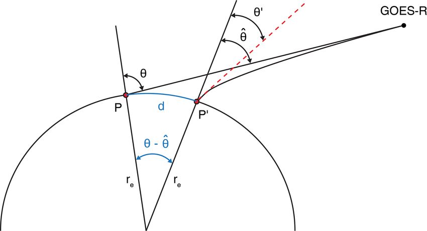
Á. Horváth et al.: Geometric estimation of volcanic eruption column height – Part 1                                         12195

method in stereo mode implies the assumptions that (i) the        the distance between the plume edge and the shadow edge
satellite images are perfectly time synchronized and (ii) the     along the azimuth φD . If the image is in a non-conformal
two look vectors, which connect the projected plume loca-         map projection, these angles are not preserved locally.
tions to the corresponding satellites, have an exact intersec-       The equirectangular projection (Plate-Carrée), used in
tion point. If the images are asynchronous, plume advection       NASA Worldview and also implicit in the gridded CEReS
between the acquisition times has to be corrected for. Fur-       AHI data, is a non-conformal projection that has a constant
thermore, look vectors never intersect in practice due to pixel   meridional scale factor of 1 but a parallel (zonal) scale factor
discretization and image navigation uncertainties. Therefore,     that increases with latitude φ as sec (ϕ). The non-isotropic
dedicated stereo algorithms use vector algebra to search for      scale factor leads to considerable east–west stretching and
the height that minimizes the distance between the passing        azimuth distortion at the latitudes of Kamchatka and the
look vectors rather than rely on the analytical solution de-      Kuril Islands. The magnitude of angular distortion depends
rived from view zenith and azimuth angles with the assump-        on azimuth and can easily be 10◦ . Angular distortion has to
tion of exact line intersection.                                  be considered, or a locally conformal map projection needs
   In Part 2 (Horváth et al., 2021), we use both the shadow-      to be used when applying methods 1–3.
stereo method and a dedicated stereo code for validation.
The analytical solution of method 3 is applied to plume top
features that could be visually identified in both GOES-17        4     Side view method
and Himawari-8 images. Limb imagery is generally unsuit-
                                                                  4.1    Measurement principle
able for automated stereo calculations due to the difficulty of
pattern matching between an extreme side view and a less          This method is essentially the same as method 1, but instead
oblique view. A human observer, however, can still identify       of calculating linear distances in a conventional map pro-
the same plume top feature even in such widely different          jection, it determines the angular extent of an eruption col-
views.                                                            umn from the ABI fixed grid image. Operating in the angular
   We also use a novel fully automated stereo code to re-         space of the fixed grid has the advantages of (i) working with
trieve plume heights of the 2019 Raikoke eruption. This           a more natural, less distorted view of a protruding column
“3D Winds” algorithm, which was originally developed              (e.g., no zonal stretching), (ii) the VIFOV being considerably
for meteorological clouds, combines geostationary imagery         smaller than the GIFOV, and (iii) no Earth curvature effects.
from GOES-16, GOES-17, or Himawari-8 with polar-orbiter           The geostationary side view geometry of the measurement is
imagery from the Multiangle Imaging SpectroRadiometer             sketched in Fig. 4. In the following we ignore atmospheric
(MISR) or Moderate Resolution Imaging Spectroradiome-             refraction effects, which will be shown to be largely negligi-
ter (MODIS) to derive not only plume height but also the          ble in Sect. 4.2.
horizontal plume advection vector (Carr et al., 2018, 2019;          The satellite coordinate system has its origin located at the
Horváth et al., 2020). The technique requires a triplet of con-   satellite’s center of mass. The x axis (Sx ) points from the
secutive geostationary full disk images and a single MISR         satellite to the center of the Earth, and the upward-pointing
or MODIS granule. Feature templates are taken from the            z axis (Sz ) is parallel to the line connecting the center of the
central repetition of the geostationary triplet and matched to    Earth with the North Pole. The y axis (Sy ) is aligned with
the other two repetitions 10 min before and after, providing      the equatorial axis and completes the right-handed coordi-
the primary source of plume velocity information. The geo-        nate system.
stationary feature template is then matched to the MISR or           The look vectors connecting the satellite to base B
MODIS granule which is observed from a different perspec-         and to the ellipsoid projected location of top
tive, providing the stereoscopic height information. The ap-                                                           T , which
                                                                  is P , are respectively       S B = S B,x B,y B,z and S P =
                                                                                                           , S   , S
parent shift in the pattern from each match, modeled pixel
                                                                   SP ,x , SP ,y , SP ,z . For convenience, Fig. 4 depicts an erup-
times, and satellite ephemerides feed the retrieval model to      tion column on the meridian of the sub-satellite point and
enable the simultaneous solution for a horizontal advection       thus plots the ellipsoidal cross section along the Sx –Sz plane.
vector and its geometric height.                                  In the general case, the shown cross section corresponds to
                                                                  the cutting plane defined by the Sx axis and look vector S B ,
3.5   Note on potential azimuth distortions in mapped             which is obtained by rotating the Sx –Sz plane around the Sx
      satellite images                                            axis by the geocentric colatitude. The image location of B is
                                                                  determined from the known geodetic latitude and longitude
At this point, it is worthwhile to note the possibility of an-    of the volcano. Calculation of the satellite-to-pixel look vec-
gular distortions in a map-projected satellite image, because     tor and the geodetic latitude and longitude of a given ABI
this caveat is usually ignored in geometric height retrievals.    image pixel is described in Appendix A.
Methods 1 and 2 require respectively the sensor-projected
column length along the view azimuth φ and the shadow
length along the solar azimuth φ0 , while method 3 requires

https://doi.org/10.5194/acp-21-12189-2021                                       Atmos. Chem. Phys., 21, 12189–12206, 2021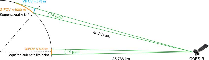
12196 Á. Horváth et al.: Geometric estimation of volcanic eruption column height – Part 1
Figure 4. Side view geometry of a vertical column located near the limb as imaged by a geostationary sensor.
The angle δ between the top and base look vectors can be – is a good choice for T (see the top middle inset in Fig. 4).
determined from the dot product of S B and S P as Under strong winds, a point near the windward plume edge
might be used instead. The approximate nature of locating
SB · SP the plume point with the smallest radial distance to the vent,
δ = acos . (9)
|S B | |S P | however, introduces an inevitable uncertainty in the height
If δ is expressed in radians, an estimate of column height h estimate.
can be obtained simply as In contrast, the tilt of the eruption column relative to Ẑ in
the Ẑ − S B × Ẑ plane can be corrected for (see the top right
ĥ = δ |S B | . (10) inset in Fig. 4). The sideways tilt angle β can be determined
from the dot product of Ẑ and vector V B T̃ connecting base
This estimate is the projection of the column height to the B to T̃ :
axis Ẑ, which is perpendicular to look vector S B and tilted
slightly from the local vertical axis Z by an angle of 90◦ − θ . Ẑ · V B T̃
The projection of T onto the Ẑ − S B × Ẑ plane by look vec- β = acos , (11)
tor S P is point T̃ . The foreshortening due to the slight rota- Ẑ V B T̃
tion from the exact limb (θ = 90◦ ) can be corrected by divid-
where
ing ĥ by cos(90◦ − θ ), which is an almost trivial correction
of 154 m/10 km at θ = 80◦ and 55 m/10 km at θ = 84◦ . Note Ẑ = S B − hsat + req − |V CB | tan 90◦ − θ , 0, 0 ,
that the angular distance between the geodetic zenith and the
V CB = S B − hsat + req , 0, 0 ,
geocentric zenith (or the angle of the vertical) equals the dif-
|S B |
ference between the geodetic latitude and the geocentric lat- V B T̃ = S P − SB . (12)
itude, which is ∼ 0.18◦ for Kamchatka. This is a negligible |S P |
difference for our purposes, and thus axis Z can be either the Here hsat = 35 786 023 m is the satellite (perspective point)
geodetic or the geocentric vertical. height above the ellipsoid, req = 6 378 137 m is the semi-
The horizontal expansion of the plume top in the radial di- major axis of the GRS80 ellipsoid, and vector V CB connects
rection, or equivalently the radial tilt of an eruption column the center of the ellipsoid to base B. The final height estimate
with no umbrella cloud, can however introduce substantial is then obtained as
biases. Expansion of the umbrella cloud towards the limb cos(β)
(away from the satellite), depicted by red in Fig. 4, leads to ĥf = ĥ . (13)
an overestimated angle δ+ between the base and top look cos (90◦ − θ )
vectors and positive height bias. Conversely, plume expan- In the actual implementation of the algorithm, we up-sample
sion away from the limb (towards the satellite), depicted by ABI images by a subpixel factor (SPF) of 2 using bilin-
blue in Fig. 4, leads to an underestimated δ− and negative ear interpolation. This follows the exact practice of the op-
height bias. To minimize such biases for an expanded um- erational ABI image navigation and registration assessment
brella cloud, one has to estimate the plume point closest to tool, which also refines ABI images to half a pixel resolu-
the vertical at the vent and use that as point T in the cal- tion (Tan et al., 2019). Here it is relevant to note that the na-
culations. If under weak winds the plume expansion is fairly tive spatial sampling by the ABI detectors (10.5–12.4 µrad) is
isotropic and advection is small, the center of the plume – de- finer than the pixel resolution (14 µrad) of the level 1B prod-
termined visually or by fitting a circle to the umbrella cloud uct (Kalluri et al., 2018). Strictly for visual clarity, images in
Atmos. Chem. Phys., 21, 12189–12206, 2021 https://doi.org/10.5194/acp-21-12189-2021Á. Horváth et al.: Geometric estimation of volcanic eruption column height – Part 1 12197
culation of the apparent horizontal displacement of the ob-
served point, i.e., the distance between P 0 and P , however,
the zenith angle difference θ − θ̂ is needed.
The calculations by Noerdlinger (1999) for “white light”
(0.46–0.53 µm), sea level, a surface temperature of 15 ◦ C,
and a refractive index at the surface of µ = 1.000290 yield a
linear displacement of 448 m at θ = 80◦ and a range of 1267–
4858 m at θ = 83◦ –86◦ typical for Kamchatka and the Kuril
Islands; these numbers could vary by ∼ 25 % depending on
weather. Using the Ciddor (1996) equation for the refractive
index – which is the current standard and is a function of
wavelength, temperature, pressure, humidity, and CO2 con-
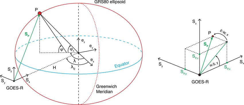
Figure 5. Terrestrial refraction geometry following No- tent – slightly reduces the surface refractive index at 0.64 µm
erdlinger (1999). The distant observer (GOES-R) views point
to µ = 1.000277 and the original Noerdlinger (1999) dis-
P 0 , which is displaced by distance d and registered in the satellite
image at point P . Noerdlinger (1999) provides analytical formulas
placement values by a few dozen to a few hundred meters.
that relate the known zenith angle θ of the unrefracted ray to θ̂ and Considering that the band 2 GIFOV (or ground sample dis-
θ 0 , from which the horizontal displacement along the surface can be tance) rapidly increases near the limb and reaches ∼ 4 km at
calculated using the local Earth curvature radius re (= 6 371 000 m θ = 84◦ , the horizontal displacement due to refraction could
in the spherical model). be a relatively modest 1–2-pixel shift at the surface.
More importantly, however, the horizontal displacement of
the surface base point does not affect our height estimates, as
subsequent figures are magnified further; however, all height long as ABI pointing and angular sampling are stable, be-
calculations are performed on data up-sampled with SPF = 2. cause the pixel location of B is fixed by the known geode-
tic latitude–longitude of the volcano rather than by search-
4.2 Refraction effects ing for the (potentially shifted) position of the volcano’s fea-
ture template within the full disk image. The height calcu-
The geometry of terrestrial refraction is sketched in Fig. 5. lation is only affected by a shift in the position of top T ,
For spaceborne observations, the known quantity is the un- because T has to be located in the image by visual means.
refracted view zenith angle of a pixel, which is the zenith The refractive displacement scales as (µ − 1.0), which in
angle at the intersection of the idealized (prolonged exoat- turn is approximately proportional to pressure. Therefore,
mospheric) ray with the Earth ellipsoid (point P ). An actual the linear displacement at 5 km altitude (∼ 500 hPa) is about
outgoing ray ascending through the atmosphere is refracted half of the surface value and less than a third of that at the
away from the zenith; hence, its zenith angle increases with tropopause. This amounts to a practically negligible subpixel
height as it slightly bends toward the satellite sensor. Conse- shift for plume tops above 5 km. For plume tops below 5 km,
quently, the apparent image position of the terrestrial source one might apply a general 1-pixel radial shift away from the
of the ray is displaced in the radial direction to a point with limb; such a first-order correction works well for the Kam-
a larger (unrefracted) view zenith angle, that is, closer to the chatka volcanic peaks we use in the next section to validate
limb (i.e., from point P 0 to point P ). A grazing ray traverses the height retrieval technique.
a substantial range in latitude and/or longitude and is sub- We note that refraction is not considered in the operational
ject to fluctuations in weather, which are complicated to han- ABI image navigation, because its effect has been deemed
dle properly. Most Earth remote sensing applications, how- marginal compared to the variation of measured geoloca-
ever, can rely on the analytical treatment of refraction by No- tion errors (Tan et al., 2019). We also note for completeness
erdlinger (1999), which was designed to derive corrections to that refraction changes the apparent solar zenith angle at low
geolocation algorithms. sun and thus also affects the shadow-based height estimation
This method assumes a spherical Earth and spherically methods through tan θ0 . In this case, the relevant quantity is
symmetric atmosphere and relates three different angles by the angle difference θ0 − θ 0 0 , which is ∼ 0.19◦ at θ0 = 84◦ ,
simple analytical formulas: the known zenith angle θ of the causing a relatively small ∼ 300 m/10 km underestimation.
unrefracted ray at surface point P , the zenith angle θ̂ of the
same unrefracted ray at the vertical of the true (refracted) 4.3 Validation using volcanic peaks
Earth intersection point P 0 , and the zenith angle θ 0 of the
refracted ray at surface point P 0 . (In the notation of No- Volcanic peaks in the Kuril Islands and Kamchatka provide
erdlinger (1999) these angles are respectively z0 , z, and z0 .) a large set of static targets for the validation of the side view
In general, θ > θ̂ > θ 0 . For the calculation of the bidirec- height estimation method. Figure 6 exemplifies the GOES-17
tional reflectance distribution function, the zenith angle dif- fixed grid view of central Kamchatka on two different days,
ference θ − θ 0 is the relevant refraction effect. For the cal- when several volcanic peaks were clearly visible. The im-
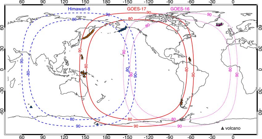
https://doi.org/10.5194/acp-21-12189-2021 Atmos. Chem. Phys., 21, 12189–12206, 202112198 Á. Horváth et al.: Geometric estimation of volcanic eruption column height – Part 1 Figure 6. GOES-17 band 2 fixed grid image of central Kamchatka on (a) 13 June 2020 at 23:00 UTC and (b) 21 December 2019 at 23:50 UTC with the most prominent volcanic peaks labeled. The images were magnified by a factor of 3, rotated clockwise by 31◦ to ensure a horizontal limb, and an inverted black–white gradient map was applied to panel (b) to mimic a shaded relief effect. ages demonstrate that viewing conditions, what astronomers base pixel and every single image pixel as described in call “seeing”, can vary significantly from day to day and even Sect. 4.1. In practice, this amounts to determining the inter- diurnally, because of changing turbulence, lighting, and hazi- section of a given pixel’s look vector and the plane that con- ness. Therefore, a given mountain peak can easily be identi- tains the base point and is perpendicular to the base pixel’s fied on certain days but not on others. look vector (i.e., the Ẑ − S B × Ẑ plane in Fig. 4). The visu- Figure 7 shows magnified views of three volcanoes of ally identified top pixel is located correctly between the 3 and increasing summit elevation: Alaid (2339 m), Kronotsky 4 km contour lines. (3528 m), and Kamen (4619 m). Here the base point (red di- The GOES-17 image in the traditional equirectangular amond) was fixed by the geodetic coordinates of the vent, projection is plotted in Fig. 8b. The mapped image is severely while the peak position (blue diamond) was visually deter- distorted compared to the natural fixed grid view, as it is mined and then corrected for refraction by applying a 1-pixel stretched in the parallel (east–west) direction by a factor inward radial shift; that is, the top pixel T used in the height of sec(ϕ = 54.75◦ ) = 1.73. This makes image interpretation calculations is the one located 1 pixel “below” the visual and the precise identification of the peak more difficult. The peak in the rotated images. Note that the distance between non-isotropic scale factor also leads to considerable azimuth the base and peak pixel increases with increasing summit el- distortions. Although the true GOES-17 view azimuth is evation. Figure 7c also highlights that identification of peaks φ = 113◦ , the mapped image of the volcano lies along the is often the easiest when the volcanoes peek through a lower apparent (distorted) azimuth of φ = 103◦ . The ellipsoid pro- level cloud layer. jected distance between the base and our best visual estimate Figure 8 demonstrates the height estimation through the peak location is ∼ 31 km, which yields a height of 3768 m us- example of Kronotsky. Using the marked base and top pix- ing Eq. (1) with a view zenith angle of θ = 83.07◦ . Although els, the side view method yields a height estimate of 3548 m, the height estimate is fairly decent in this particular case, the which is in excellent agreement with the true height of severe image distortions make height calculation from linear 3528 m. Figure 8a shows the fixed grid view with base- distances measured in a conventional map projection gener- relative isoheight lines drawn as visual aid. These contour ally inferior to the angular technique facilitated by the fixed lines were obtained by calculating the height between the grid side view. Atmos. Chem. Phys., 21, 12189–12206, 2021 https://doi.org/10.5194/acp-21-12189-2021
Á. Horváth et al.: Geometric estimation of volcanic eruption column height – Part 1                                                   12199

Figure 7. GOES-17 band 2 fixed grid image after 8× magnification of (a) Alaid (Atlasov Island, 2339 m) on 30 March 2020 at 00:00 UTC,
(b) Kronotsky (3528 m) on 13 June 2020 at 23:00 UTC, and (c) Kamen (4619 m) on 8 April 2020 at 19:00 UTC. The image pixel correspond-
ing to the geodetic latitude–longitude of the vent is marked by a red diamond. The visually identified peak with a 1-pixel radial refraction
correction applied is marked by a blue diamond. The images were rotated clockwise by the geodetic colatitude angle. In panel (c), the tops
of (left to right or south to north) Kamen, Ushkovsky (3891 m), Klyuchevskoy (4835 m), and Krestovsky (4048 m) are seen peeking through
the cloud layer.

Figure 8. GOES-17 band 2 image of Kronotsky (3528 m) on 13 June 2020 at 23:00 UTC in (a) fixed grid projection (8× magnification)
and (b) equirectangular (Plate-Carrée) projection. In panel (a), the red and blue diamonds mark the volcano base and peak, respectively, and
the horizontal lines are base-relative isoheights drawn at 1 km intervals (solid green: surface, cyan dotted: odd numbers, yellow dotted: even
numbers). In panel (b), the green quadrilateral bounds the area shown in panel (a), the red triangle indicates the volcano base, and the cyan
curve is the coastline. The true view azimuth (φ = 113◦ ), the apparent (distorted) azimuth (φ = 103◦ ), and the ellipsoid-projected distance
between the base and peak locations are also indicated.

   For a more comprehensive validation, we selected 50                   mits and is based on DEMs from the European Copernicus
mountain peaks ranging in elevation from 502 m (Mashkovt-                program, the United States Geological Survey (USGS), and
sev) to 4835 m (Klyuchevskoy). The geodetic latitude–                    the Japan Aerospace Exploration Agency (JAXA).
longitude and the elevation of a given peak can differ slightly             The name, geodetic latitude and longitude, true height, and
between databases (Global Volcanism Program, Google                      estimated height of the selected peaks, as well as the date
Earth, KVERT list of active volcanoes), due mainly to the use            and time of the GOES-17 images used, are listed in Table S1
of different reference ellipsoids (the exact choice of which,            in the Supplement. As previously discussed, the observing
however, is usually undocumented). For example, the eleva-               conditions show considerable temporal variation, but for a
tion of Kronotsky is 3482 m in the Global Volcanism Pro-                 static target one has the luxury of a large number of avail-
gram database and 3528 m in the KVERT list. In our work,                 able images from which to choose one that offers a good
we relied on PeakVisor (https://peakvisor.com, last access:              view of the peak. For a volcanic plume, one is limited to a
10 August 2021), which is one of the most advanced moun-                 few images around the eruption time; however, identifying a
tain identification and 3D maps tool (also available as a mo-            high-altitude plume top is also much easier, because reduced
bile app). Its peaks database has almost a million named sum-            atmospheric turbulence and the distinct color of the ejecta

https://doi.org/10.5194/acp-21-12189-2021                                                Atmos. Chem. Phys., 21, 12189–12206, 2021
12200                                     Á. Horváth et al.: Geometric estimation of volcanic eruption column height – Part 1

                                                                         other height retrieval methods, is given in Part 2 (Horváth
                                                                         et al., 2021). The Sheveluch volcano has three main ele-
                                                                         ments: Old Sheveluch with an elevation of 3307 m, the old
                                                                         caldera, and the active Young Sheveluch with a lava dome
                                                                         at 2589 m surrounded by peaks of about 2800 m elevation.
                                                                         A strong explosive eruption occurred on 8 April 2020 at
                                                                         19:10 UTC, slightly after sunrise, whose ash plume advected
                                                                         south-southeast from Young Sheveluch. The Kamchatka Vol-
                                                                         canic Eruption Response Team issued an orange-coded Vol-
                                                                         cano Observatory Notice for Aviation (VONA 2020-40,
                                                                         http://www.kscnet.ru/ivs/kvert/van/?n=2020-40, last access:
                                                                         10 August 2021), reporting a plume height of 9.5–10.0 km as
                                                                         determined by the basic satellite temperature method from
                                                                         Himawari-8 11 µm data.
                                                                            The GOES-17 fixed grid images capturing the eruption
                                                                         are presented in Fig. 10. Figure 10a shows the volcano at
                                                                         19:00 UTC before the eruption, with the volcanic peaks, es-
                                                                         pecially the more northerly Old Sheveluch, clearly recogniz-
Figure 9. Peak height estimated by the side view method versus
true peak height; two different colors and symbols are used only to
                                                                         able above a low-level stratus layer. Faraway peaks of the
help distinguish overlapping data points. The dashed line is the 1 : 1   Sredinny Mountain Range west of Sheveluch can also be
line, and the dotted lines mark ±2× RMSE about the 1 : 1 line. The       seen in the background. By the time of the next full disk
error bars on a data point represent the standard deviation of the       image acquired at 19:10 UTC and depicted in Fig. 10b, the
nine height estimates corresponding to the visually identified peak      eruption column reached its maximum altitude and devel-
location and its 8-pixel neighborhood.                                   oped a small umbrella cloud, which was advected slightly to
                                                                         the south-southeast by the prevailing upper-level winds. No-
                                                                         table features in this image are a portion of the long shadow
usually lead to good contrast against the background. The                cast by the ash column and the brighter sunlit near side (east-
height error estimates obtained below for volcanic peaks un-             ern edge) and the darker shadowed far side (western edge) of
der good “seeing”, nevertheless, represent a lower limit, be-            the umbrella cloud, brought out by the rising sun in the east
cause the (typically unknown) radial tilt of eruption columns            (θ0 = 86.0◦ , φ0 = 82.6◦ ).
introduces additional uncertainty in the retrievals.                        A simple technique commonly applied to aid change
   The scatter plot of estimated peak height versus true peak            detection in multitemporal imagery is the computation
height is given in Fig. 9 (remember, ABI images are up-                  of running-difference images. The normalized running-
sampled with SPF = 2). For each data point, we performed                 difference (RD) image at time t can be defined as
a sensitivity analysis by shifting the visually determined                                                  himaget i
peak location by ±1 pixel in either direction and calculating            imageRD,t = imaget − imaget−1                 ,           (14)
                                                                                                           himaget−1 i
heights for the central pixel and its 8-pixel neighborhood.
The standard deviation of these nine height values is then               where “image” is a 2D array of reflectances and h i indicates
used as an error bar. The root mean square error (RMSE)                  the mean of all pixels. The advantage of such a running-
computed for the 50 peaks corresponds to the unperturbed                 difference image, whose mean pixel value is ∼ 0, is that
best estimate peak locations. As shown, the overall bias is              static or quasi-static background features are removed, mak-
a negligible 28 m and the RMSE is 150 m. The error bar                   ing identification of dynamic features easier. The RD image
on individual retrievals is ∼ 250 m, with a maximum pos-                 calculated from the 19:10 and 19:00 UTC GOES-17 snap-
sible height discrepancy of ±400 m due to a 1-pixel uncer-               shots is plotted in Fig. 10c. Note how the plume and its
tainty in peak location; these numbers increase to ∼ 300 m               shadow are accentuated, while Old Sheveluch and the peaks
and ±500 m when ABI images are used without up-sampling                  of the Sredinny mountains are removed in this image. Simi-
(SPF = 1). We conclude from these results that in the absence            lar or more sophisticated image change detection algorithms
of significant radial tilt, ±500 m is a reasonable uncertainty           (Radke et al., 2005) could later be used for the automated
value for instantaneous height retrievals.                               detection of volcanic eruptions in side view imagery, where
                                                                         traditional methods based on brightness temperature differ-
4.4   Sheveluch eruption on 8 April 2020                                 ences might be problematic due to the extreme view geome-
                                                                         try (e.g., limb darkening or brightening effects).
As a final example in Part 1, we demonstrate the side view                  Finally, Fig. 10d presents the fixed grid view of the plume
method on the 8 April 2020 eruption of Sheveluch. A de-                  at 19:10 UTC with the base-relative isoheight lines drawn.
tailed analysis of this case, including a comparison with                The summit of Old Sheveluch is correctly located between

Atmos. Chem. Phys., 21, 12189–12206, 2021                                                https://doi.org/10.5194/acp-21-12189-2021
Á. Horváth et al.: Geometric estimation of volcanic eruption column height – Part 1 12201
Figure 10. GOES-17 band 2 fixed grid image (8× magnification) of Young and Old Sheveluch (2589 and 3307 m, respectively) on
8 April 2020 at (a) 19:00 UTC, (b) 19:10 UTC, and (c) 19:10 UTC running-difference image, as well as (d) 19:10 UTC with base-relative
isoheight lines drawn at 1 km intervals. The images were rotated clockwise by the geodetic colatitude angle. The red diamond marks the base
of the active Young Sheveluch, and the blue diamond indicates our best visual estimate plume top position above the vent.
the 3 and 4 km contour lines. Our best estimate plume top using data from the ABI instrument, which offers the highest-
position directly above the vent is marked by the blue dia- resolution visible imagery and most accurate georegistration
mond, which was visually determined considering the expan- among current-generation geostationary imagers. The pub-
sion and slight advection of the umbrella cloud and which licly available ABI level 1B data distributed by NOAA also
lies halfway between the far-side and near-side edges. The contain all the information required for the calculations.
selected top pixel leads to a plume height estimate of ∼ 8 km. Thanks to its purely geometric nature, the technique avoids
Note that the radial expansion of the plume at an approxi- the pitfalls of the traditional brightness temperature method;
mately constant altitude results in height biases as sketched however, it is mainly applicable to strong eruptions with
in Fig. 4. The darker far-side edge of the umbrella, which is nearly vertical columns, and its coverage is limited to day-
located behind the plane of the isoheights, appears at an al- time point estimates in the immediate vicinity of the vent.
titude of ∼ 9 km, while the brighter near-side edge, which is Initial validation of the technique on mountain peaks in Kam-
located in front of the isoheights’ plane, appears at ∼ 7 km. chatka and the Kuril Islands indicates that ±500 m is a rea-
In contrast, the latitudinal (left–right) expansion of the plume sonable preliminary uncertainty value for height estimates of
has little effect on the height estimates. The side view plume near-vertical eruption columns; this uncertainty compares fa-
height of ∼ 8 km is 1.5–2.0 km lower than the height from vorably with the 2–4 km uncertainty typical of state-of-the-
the temperature method, and, based on the discussion above, art radiometric methods. The radial expansion of the volcanic
we think it is closer to the true plume altitude. This dis- umbrella cloud or the radial tilt of a weak eruption column
crepancy, caused by well-known retrieval biases near the under strong wind shear, however, introduces additional er-
tropopause temperature inversion, is further investigated in rors that need further characterization. In Part 2 of the paper,
Part 2 (Horváth et al., 2021). we apply the technique to seven recent volcanic eruptions
observed by GOES-17 in Kamchatka, the Kuril Islands, and
Papua New Guinea, including the 2019 Raikoke eruption,
5 Summary and compare the side view plume height estimates with those
from the IR temperature method, stereoscopy, and ground-
We presented a simple geometric technique that exploits the
based video camera and quadcopter images.
generally unused near-limb portion of geostationary fixed
grid images to estimate the height of a volcanic eruption col-
umn. Such oblique angle observations provide an almost or-
thogonal side view of a vertical column protruding from the
Earth ellipsoid and allow height calculation by measuring the
angular extent of the column. We demonstrated the technique
https://doi.org/10.5194/acp-21-12189-2021 Atmos. Chem. Phys., 21, 12189–12206, 2021You can also read