Fine-scale vertical structure of sound-scattering layers over an east border upwelling system and its relationship to pelagic habitat ...
←
→
Page content transcription
If your browser does not render page correctly, please read the page content below
Ocean Sci., 16, 65–81, 2020
https://doi.org/10.5194/os-16-65-2020
© Author(s) 2020. This work is distributed under
the Creative Commons Attribution 4.0 License.

Fine-scale vertical structure of sound-scattering layers over an east
border upwelling system and its relationship to pelagic
habitat characteristics
Ndague Diogoul1,2,6 , Patrice Brehmer2,3,6 , Yannick Perrot3 , Maik Tiedemann4 , Abou Thiam1 ,
Salaheddine El Ayoubi5 , Anne Mouget3 , Chloé Migayrou3 , Oumar Sadio2 , and Abdoulaye Sarré6
1 University  Cheikh Anta Diop UCAD, Institute of Environmental Science (ISE), BP 5005, Dakar, Senegal
2 IRD,  Univ. Brest, CNRS, Ifremer, LEMAR, Campus UCAD-IRD de Hann, Dakar, Senegal
3 IRD, Univ. Brest, CNRS, Ifremer, LEMAR, DR Ouest, Plouzané, France
4 Institute of Marine Research IMR, Pelagic Fish, P.O. Box 1870 Nordnes, 5817 Bergen, Norway
5 Institut National de Recherche Halieutique INRH, Agadir, Morocco
6 Institut Sénégalais de Recherches agricoles ISRA, Centre de Recherches Océanographiques de Dakar-Thiaroye (CRODT),

BP 2221 Dakar, Senegal

Correspondence: Ndague Diogoul (diogoulndague@yahoo.fr)

Received: 12 March 2019 – Discussion started: 8 April 2019
Revised: 20 November 2019 – Accepted: 25 November 2019 – Published: 13 January 2020

Abstract. Understanding the relationship between sound-          vertical migration boundary. The results increase the under-
scattering layers (SSLs) and pelagic habitat characteristics     standing of the spatial organization of mid-trophic species
is a substantial step to apprehend ecosystem dynamics. SSLs      and migration patterns of zooplankton and micronekton, and
are detected on echo sounders representing aggregated ma-        they will also improve dispersal models for organisms in up-
rine pelagic organisms. In this study, SSL characteristics of    welling regions.
zooplankton and micronekton were identified during an up-
welling event in two contrasting areas of the Senegalese con-
tinental shelf. Here a cold upwelling-influenced inshore area
was sharply separated by a strong thermal boundary from a
deeper, warmer, stratified offshore area. Mean SSL thickness     1   Introduction
and SSL vertical depth increased with the shelf depth. The
thickest and deepest SSLs were observed in the offshore part     Aggregations of marine pelagic organisms in ocean water can
of the shelf. Hence, zooplankton and micronekton seem to         be observed acoustically as sound-scattering layers (SSLs)
occur more frequently in stratified water conditions rather      (Evans and Hopkins, 1981; Cascão et al., 2017). The SSLs
than in fresh upwelled water. Diel vertical and horizontal mi-   represent a concentrated layer of marine organisms such as
grations of SSLs were observed in the study area. Diel period    zooplankton aggregates and nekton that occur at specific
and physicochemical water characteristics influenced SSL         depths (Benoit-Bird and Au, 2004). Nevertheless, the SSL is
depth and SSL thickness. Although chlorophyll-a concen-          not a biological classification, and animals making up SSLs
tration insignificantly affected SSL characteristics, the peak   include various species, with correspondingly different bio-
of chlorophyll a was always located above or in the mid-         logical, physiological, and ecological needs. The SSLs are
dle of the SSLs, regularly matching with the peak of SSL         dynamic, active, and have a particular behavior as a function
biomass. Such observations indicate trophic relationships,       of their community structure, causing changes in their verti-
suggesting SSLs to be mainly composed of phytoplanktiv-          cal distribution, size, and shape over time and space (Gómez-
orous zooplankton and micronekton. Despite local hypoxia,        Gutiérrez et al., 1999). Zooplanktonic and micronektonic
below 30 m depth, distribution patterns of SSLs indicate no      components are fundamental to ecosystem functioning, par-

Published by Copernicus Publications on behalf of the European Geosciences Union.
66             N. Diogoul et al.: Sound-scattering layers structure and its relationship to pelagic habitat characteristics

ticularly in productive upwelling areas (e.g., off the south      in zooplankton and micronekton. Many zooplankton groups
coast of Senegal).                                                are encountered over the Senegalese coastal shelf: Cope-
   Zooplanktonic and micronektonic species provide the            pods, amphipods, annelids, appendicularians, chaetognaths,
main trophic link between primary producers and higher            cirrhipeds, cladocerans, Decapoda, echinoderms, euphausi-
trophic levels. A large amount of energy passes through zoo-      ids, gasteropods, jellyfish, Mysidacea, ostracods, pelagic
plankton and micronekton (Steele et al., 2007). Knowledge         foraminifera, Protozoa, pteropods, and Spumellaria. Cope-
of the vertical structure of SSLs allows us to understand their   pod is the most dominant group with a total abundance rang-
role in ecosystems, information that can be used to monitor       ing from 50 % to 90 % (Anonymous, 2013; Ndour et al.,
major environmental change and variability. Most zooplank-        2018; Touré, 1971). Previous studies (Ndour et al., 2018;
ton and micronektonic taxa undergo diel vertical migration        Tiedemann and Brehmer, 2017) on ichthyoplankton showed
(DVM), meaning that they reside in deep waters during the         that Sparidae (∼ 50 %) was predominant, followed by fewer
day and migrate toward the surface at night to feed (Bianchi      Engraulidae (∼ 8 %) and Soleidae (∼ 7 %), while smaller
et al., 2013; Lehodey et al., 2015). DVM behaviors are in-        proportions of Clupeidae and Carangidae (∼ 4 % each) as
fluenced by environmental cues (e.g., light, nutrients, and       well as Myctophidae and Sciaenidae (∼ 2 % each) were
temperature) and predator–prey interactions (Clark and Levy,      found. Physical variability in the Senegalese coastal shelf
1988; Lampert, 1989). Thus, DVMs represent an essential bi-       (Capet et al., 2016; Ndoye et al., 2017) can impact ma-
ological process in the ocean, one that also regulates the bio-   rine pelagic organisms at the individual and community level
logical carbon pump (Hidaka et al., 2001). Zooplankton and        (Urmy and Horne, 2016). Such an impact can be direct via
micronekton are also known to undergo diel horizontal mi-         advection or indirect via phytoplankton production fertil-
gration (DHM), moving them to within 1 km of the shoreline        ized by upwelled nutrients. Indeed, changes in physicochem-
each night into shallower waters (Benoit-Bird et al., 2001).      ical water properties and biological activities induced by up-
DHM, like DVM, which often occur concurrently, helps or-          welling plays a structuring role on the distribution of SSLs.
ganisms to find food and avoid predators (White, 1998).           SSL position is often reported below the thermocline, sug-
   The distribution of SSLs is influenced by a variety of en-     gesting that temperature controls the SSL’s vertical distribu-
vironmental factors (Aoki and Inagaki, 1992; Baussant et          tion (Aoki and Inagaki, 1992; Baussant et al., 1992; Boersch-
al., 1992; Dekshenieks et al., 2001; Marchal et al., 1993).       Supan et al., 2017; Marchal et al., 1993). Bottom depth has
Changes in the structure and density of SSLs is associated        been identified as an additional factor structuring the vertical
with frontal zones (Aoki and Inagaki, 1992; Baussant et           distribution of SSLs (Gausset and Turrel, 2001). For exam-
al., 1992; Boersch-Supan et al., 2017; Coyle and Cooney,          ple, the thickness and depth of an SSL on continental shelves
1993). Oceanic fronts are relatively narrow zones of en-          tend to increase with an increase in water depth (Torgersen
hanced horizontal gradients of physical, chemical, and bio-       et al., 1997), similar to patterns observed in the deep sea
logical properties (temperature, salinity, nutrients, plankton    (Berge et al., 2014; Boersch-Supan et al., 2017). In deep-
communities, etc.) that separate broader areas of different       sea areas and over shelves, the maximum density of SSLs
vertical structure (stratification) (Belkin et al., 2009). Up-    are often correlated with maximum chlorophyll-a concen-
welling fronts occur in many well-studied systems, includ-        trations (Berge et al., 2014; Dekshenieks et al., 2001; Hol-
ing the upwelling off southern Senegal, south of Cap-Vert         liday et al., 2010). Dissolved oxygen concentrations (above
peninsula known as the “Petite Côte” (14.6–13.5◦ N, 16.9–         1 mL L−1 , i.e., 44.661 mmol m−3 ) can also predict the lower
17.6◦ W). Senegalese coasts are characterized by a seasonal       boundary of SSL density, e.g., in eastern boundary upwelling
upwelling (in winter and late spring), mainly driven by wind      systems (EBUSs), like the Peruvian coastal upwelling system
variability, topography, and density stratification (Estrade      (Bertrand et al., 2010) and the California coastal upwelling
et al., 2008). During the upwelling season, northerly trade       system (Netburn and Koslow, 2015).
winds induce a strong upwelling core south of Dakar (Ndoye           In this study, we use acoustic tools (Simmonds and
et al., 2014; Roy, 1998). The upwelling core is located over      MacLennan, 2005a) to examine the fine-scale vertical struc-
the shelf, and SST (sea surface temperature) is lowest on         ture of SSLs (i.e., their depth in the water column, thickness,
the coastal side of the shelf break, increasing in both off-      and density) (Bertrand et al., 2013; Perrot et al., 2018). We
shore and coastal directions. Local bottom relief combined        use fine spatiotemporal resolution of acoustic data to inves-
with the wind-induced upwelling establishes a typical up-         tigate how the pelagic environment influences SSLs in the
welling that appears as a cold-water tongue. This cold-water      EBUS off Senegal during an upwelling event. Our objective
tongue separates the nutrient-poor warm offshore cell with a      was to model variations in SSLs structure relative to physic-
cold nutrient-rich coastal cell functioning as a retention zone   ochemical characteristics of water masses and their locations
(Roy, 1998; Tiedemann and Brehmer, 2017). The Petite Côte         on the shelf.
in the Senegalese coastal shelf is a nursery area for fish and
is the main area in which juveniles of numerous species, par-
ticularly small pelagic species, concentrate (Diankha et al.,
2018; Thiaw et al., 2017). This area is also known to be rich

Ocean Sci., 16, 65–81, 2020                                                                    www.ocean-sci.net/16/65/2020/
N. Diogoul et al.: Sound-scattering layers structure and its relationship to pelagic habitat characteristics 67
2 Materials and methods
2.1 SSLs acoustics sensing and environmental data
We performed a hydroacoustic survey along the “Petite
Côte”, south of Cap-Vert peninsula off Senegal (14.6–
13.5◦ N, 16.9–17.6◦ W). The survey was conducted with the
research vessel Antea of the French National Research In-
stitute of Sustainable Development (IRD France) during the
upwelling season from 6 to 18 March 2013. The Petite Côte
is a nursery area for fish and is the main area in which juve-
niles of numerous species (particularly small pelagic species)
concentrate (Diankha et al., 2018; Thiaw et al., 2017). Strong
upwelling occurs during spring, which contributes to high
primary productivity, thus providing an ideal nursery area
for commercially important fish species (Tiedemann and
Brehmer, 2017).
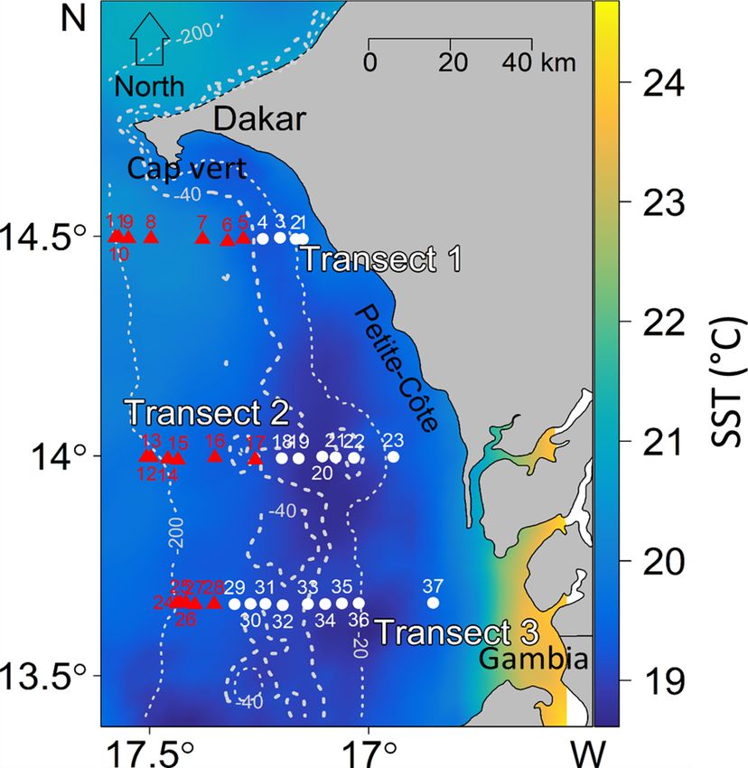
We collected hydroacoustic data along three transects (T1 Figure 1. Location of the survey area off the southern Senegalese
(North), T2 (intermediary), and T3 (south)) in 18 nautical (West African) coast. The hydroacoustic survey was conducted with
miles (nmi) perpendicular to the coast (Fig. 1). Hydroacous- FRV Antea (IRD) from Dakar (Cap-Vert peninsula) to the northern
border of Gambia. CTD probes collected data at stations along three
tic data were continuously recorded (day and night) using
transects perpendicular to the coast (T1 to T3). Sea surface temper-
a Simrad EK60 echo sounder (38, 70, 120, and 200 kHz), atures (SST, ◦ C) were averaged over the 3 d of CTD sampling from
set at 20 log R time-varied gain function (where R is the the 6 to 8 March 2013. Stations of Group 1 (white circles) were
range in meters) and using a pulse length of 1.0 ms. In this located in the inshore zone, whereas stations of Group 2 (red trian-
study, we used the acoustic monofrequency approach (us- gles) were situated further offshore. The dashed white lines repre-
ing 38 kHz, one of the most current frequencies used in fish- sent bathymetry (in meters).
eries surveys) to study the spatiotemporal SSL structure. The
38 kHz frequency offers the advantages of depth penetra-
tion, covering the whole vertical range of SSLs. The mul- rection, we extracted the SSLs that were below the mean
tifrequency echogram was used to identify the main scat- acoustic volume backscattering strength (Sv in dB) thresh-
terers of SSLs and to justify the SSLs extraction thresh- old of −75 dB (i.e., values below −75 dB were excluded
old (see below). Transducers were calibrated following the from the analysis). Cascão et al. (2017) and Saunders et
procedures recommended in Foote et al. (1987). Consider- al. (2013) excluded marine pelagic organisms that backscat-
ing the aft draught of the vessel, the acoustic near field, tered at −70 dB, a threshold based on the aggregative be-
and the presence of acoustic parasites (including air bub- havior of marine pelagic organisms. The SSL extraction
bles) in the upper part of the water column, we have ap- method is based on a threshold of −75 dB and a MAT-
plied an offset of 10 m (acoustic data above 10 m have been LAB algorithm used in Matecho named “contourf.m” (https:
deleted). Echoes along the three transects were integrated at //ch.mathworks.com/help/matlab/ref/contourf.html, last ac-
a spatial resolution of 0.1 nmi × 1 m depth. We estimated the cess: 12 January 2019), which appear relevant to extract the
SSL acoustic density by calculating the nautical area scat- main SSL at 38 kHz (Fig. S2). This process performs a seg-
tering coefficient (NASC or sA ), which represents the rela- mentation of the echo integration from the given threshold
tive biomass of acoustic targets. We assumed that the com- on echo levels to extract (by calculation of isolines accord-
position of the scattering layers and the resulting scatter- ing to the selected Sv threshold) the attached echo groups that
ing properties of organisms in the SSLs are homogeneous formed the SSLs and their associated contours. Based on this
within each layer we identified (sensu MacLennan et al., contour, a set of descriptors are estimated, e.g., up and down
2002). We analyzed integrated echoes using the in-house depths of SSL and thickness. In our study, the backscattering
tool “Matecho” (Perrot et al., 2018). Matecho is an inte- was due to zooplankton and micronekton, as well as small
grative processing software that allows us to manually cor- pelagic fish. The inshore area is known to be rich in copepod
rect echograms (e.g., by correcting bottom depths, removing and fish larva (Ndour et al., 2018; Tiedemann and Brehmer,
empty pings, removing echogram interferences, and reduc- 2017); however, a low sample number was collected in the
ing background noise). For echo-integration accuracy, Mat- coastal inshore water due to safety reasons, i.e., the research
echo computes a quality factor (QC) (Fig. S1 in the Supple- vessel investigated areas of > 20 m bottom depth.
ment) for each echo-integration cell, which is the number We collected hydrographic data using a calibrated Sea-
of integrated samples divided by the total number of sam- Bird SBE 19plus conductivity, temperature, and depth
ples in one echo-integration cell. After each echogram cor- (CTD) probe. The CTD specifications for temperature were
www.ocean-sci.net/16/65/2020/ Ocean Sci., 16, 65–81, 2020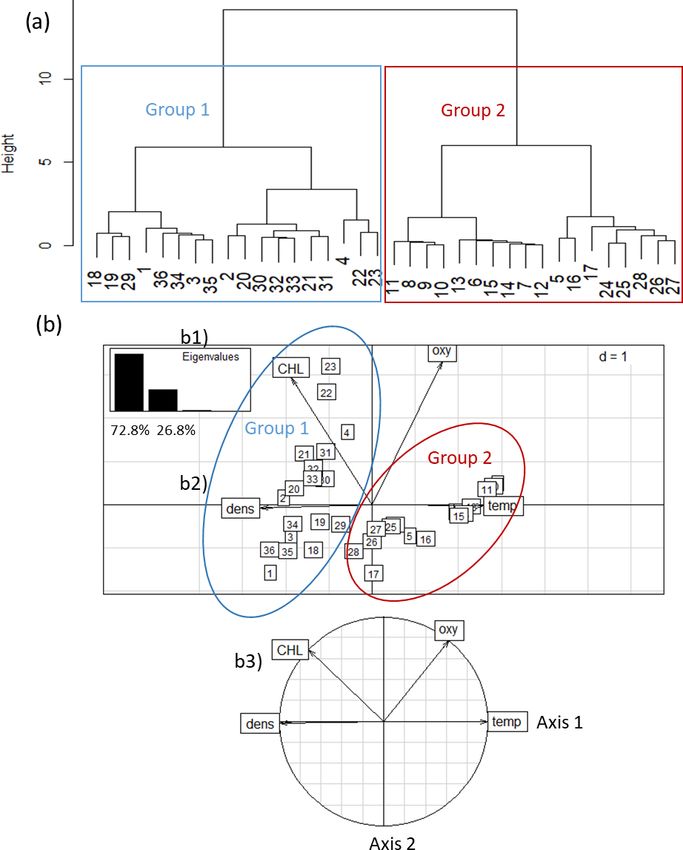
68                N. Diogoul et al.: Sound-scattering layers structure and its relationship to pelagic habitat characteristics

±5.10−3 ◦ C accuracy and 1.10−4 ◦ C precision; for conduc-                   The ComparEchoProfil displayed the profile for Sv in dB
tivity, they were ±5.10−4 S m−1 accuracy and 5.10−5 S m−1                    over an ESU of 0.1 nmi around each CTD station. The pro-
precision; for pressure, they were ±0.1 % of full-scale range                gram also allowed us to display acoustic profiles for physico-
accuracy and 2.10−3 % precision of full-scale range pre-                     chemical parameters (temperature, CHL (chlorophyll), den-
cision. The CTD was equipped with sensors for fluores-                       sity, and DO) associated with SV profiles (Fig. 2). The output
cence (±2.10−3 µg L−1 accuracy, and ±2.10−4 µg L−1 pre-                      included meta-information (station ID, station date, station
cision) (a measure of chlorophyll-a concentration, a proxy                   time, latitude and longitude, diel phase (day, night), and bot-
for phytoplankton biomass), and dissolved oxygen sensor                      tom depth), all of which we associated with SSL descriptors
(DO, mmol m−3 , Sea-Bird SBE 43, 2 % saturation for accu-                    (SSL thickness, maximum SSL depth, Sv , and sA ) based on
racy and 0.2 % saturation for precision). The CTD has been                   classic fish school descriptors (Brehmer et al., 2007, 2019)
calibrated before the survey. During the survey, data deliv-                 and physicochemical parameters associated with each SSL.
ered by the SBE 43 for DO have been corrected by Win-                           We applied hierarchical cluster analyses (HCAs) to dis-
kler titrations. From 6 to 8 March 2013, we conducted CTD                    criminate between water masses of inshore and offshore sta-
casts along three transects at 36 stations. At each station,                 tions over the continental shelf based on CTD data collected
sensors measured water temperature (◦ C), depth (m), fluo-                   at 10 m depth. HCA was based on Euclidean distance and
rescence (µg L−1 ), water density (here sigma-theta, kg m−3 ),               Ward’s aggregation method (Ward, 1963). We used principal
and DO. Global High Resolution Sea Surface Temperature                       component analysis (PCA) (Chessel et al., 2013) on the same
(GHRSST) data were extracted from daily outputs by the Re-                   dataset to determine similarities between CTD stations rela-
gional Ocean Modeling System group at NASA’s Jet Propul-                     tive to environmental parameters. Physicochemical parame-
sion Laboratory (JPL OurOcean Project, 2010). Daily SST                      ters were standardized a priori because they were measured
data (GHRSST Level 4 G1SST Global Foundation Sea Sur-                        with different metrics.
face Temperature Analysis) were averaged for the 3 d of sur-                    Inshore–offshore variability of morphometric (thickness,
veying using SeaDAS software version 7.2 (https://seadas.                    depth) and acoustic characteristics (sA ) of the SSLs are in-
gsfc.nasa.gov/, last access: 10 November 2018) and interpo-                  vestigated in the discriminated groups considering bottom
lated on maps using R software (R Core Team, 2016). Cubic                    depth and diel period. Diel transition periods are removed
spline interpolations of gridded data were used within the R                 from analyses to avoid SSL density change biases due to diel
package Akima (Akima et al., 2016).                                          vertical migrations. Transition periods are defined using sun
                                                                             altitude, i.e., around sunset and sunrise corresponding to a
2.2   Data analysis                                                          sun altitude between ±18◦ (Lehodey et al., 2015). Morpho-
                                                                             metric and acoustic characteristics of the SSLs are also com-
After extracting SSLs with Matecho, we developed an ad                       pared between the inshore area versus offshore area and be-
hoc MATLAB extension of Matecho named “Layer” (S1 in                         tween day and night using Student’s t test whose application
the Supplement). We obtained SSL thickness, minimum and                      conditions have been verified (normal distribution and vari-
maximum SSL depths (Dmin and Dmax , respectively), and                       ance equality).
an echo-integrated echogram from Matecho output files to                        Echogram vs. profile coupling figures (Fig. 2) resulting
provide it to another MATLAB program “ComparEchoPro-                         from the ComparEchoProfil were analyzed to determine the
fil” (S2). ComparEchoProfil allows the user to fit in time and               relation between environmental parameters and SSLs. AN-
depth echo-integrated echograms to the associated CTD ver-                   COVA tests (analysis of covariance) (Wilcox, 2017) were
tical profiles. We used the equation below to calculate thick-               implemented for SSL characteristics (thickness, depth, and
ness:                                                                        density) in each discriminated area (inshore and offshore).
                                                                             These models were set to predict each descriptor, i.e., thick-
Thickness = Dmax − Dmin                                                (1)   ness, depth, and sA as a function of temperature, density, DO,
                                                                             CHL, local depth, and diel period. The ANCOVA models
Mean nautical area backscattering coefficient (sA , NASC)
                                                                             were developed on averaged data over station. The selection
and mean acoustic volume backscattering strength (Sv in dB)
                                                                             of the best models was performed using stepwise procedures.
profiles were based on the average of three ESUs (small-scale
                                                                             Stepwise selection was based on minimizing the Akaike in-
elementary sampling units): the ESU nearest to the CTD po-
                                                                             formation criterion (AIC) (Akaike, 1974). The relative im-
sition (ESUctd ) as well as previous and following in corre-
                                                                             portance of each variable in total deviance explained was
spondence with CTD depths (dn )
                                                                             determined from the “relaimpo” R package (Tonidandel and
             i=ESU                                                           LeBreton, 2011). Validity assumptions of the models were
                Xctd +1
sA (dn ) =                 sA (i, dn ) /3,                             (2)   then assessed by checking for normality of distributed er-
             i=ESUctd −1                                                     rors and homogeneity of residuals (Figs. S3 to S5). For the
                             i=ESU
                                                                 !           ANCOVA, SSL density (sA ) was log10 transformed for nor-
                                Xctd +1
Sv (dn ) = 10 × log10                         (Sv (i,dn )/10)
                                             10                 /3 .   (3)   mality assumption. For all statistical tests, the significance
                             i=ESUctd −1                                     threshold used was 0.05.

Ocean Sci., 16, 65–81, 2020                                                                               www.ocean-sci.net/16/65/2020/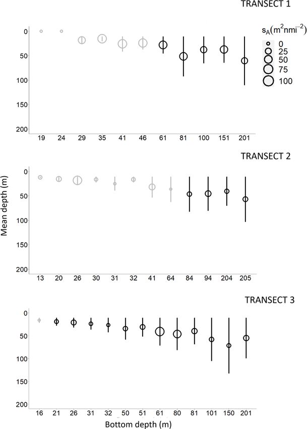
N. Diogoul et al.: Sound-scattering layers structure and its relationship to pelagic habitat characteristics 69
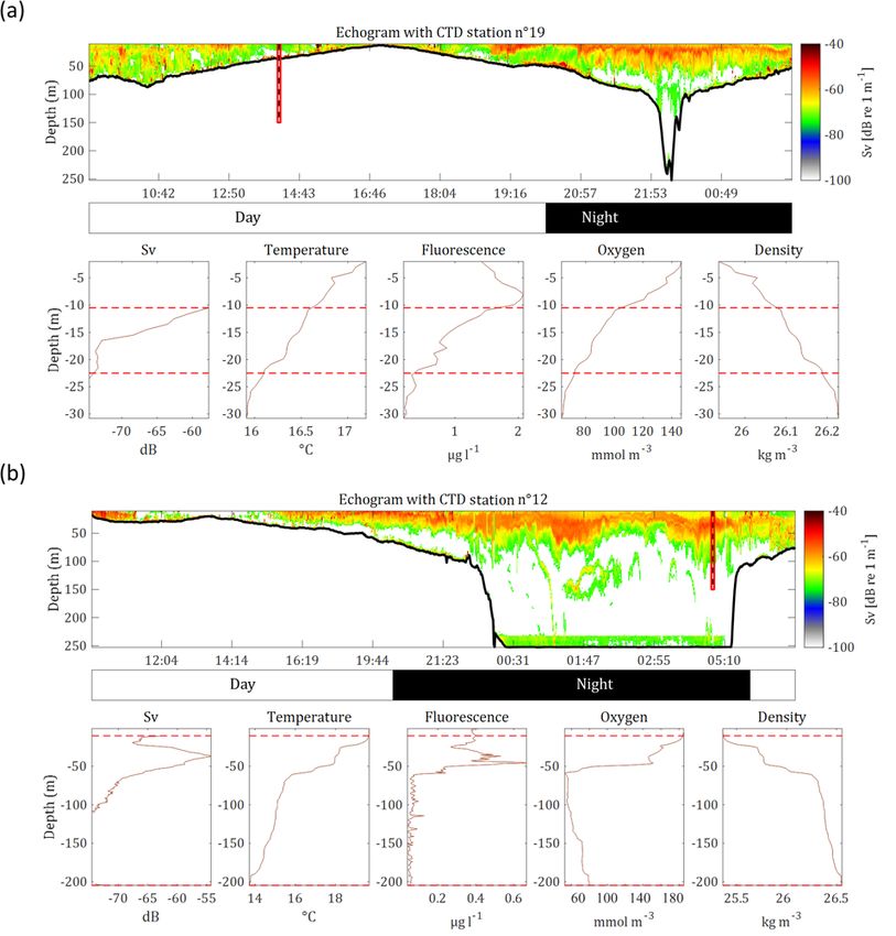
Figure 2. Echograms and associated vertical acoustic profiles as well as physicochemical parameters (CTD data) for two example stations:
(a) station 19 in the inshore area and (b) station 12 in the offshore area. For both (a) and (b), top panels are echogram data collected along the
transect, i.e., 1000 ESU (elementary sampling unit) of 0.1 nmi, whereas the bottom panels depict acoustic and environmental data (depicted
by the vertical red line in top panels). Environmental data for the sound-scattering layer (SSL) were collected at the stations at the locations
depicted by dotted vertical lines. Data represent mean conditions for the station collected within an area of 0.1 nmi around the station:
acoustic volume backscattering strength (Sv ) SSL, temperature profile SSL, CHL profile SSL, oxygen profile SSL, and density profile SSL.
The horizontal dashed lines in all profiles represent the SSL thickness, i.e., the upper and lower SSL limits.
We used R software (R Core Team, 2016) for statistical 3 Results
analyses and to map data. We used the R package “Cluster”
(Maechler et al., 2014) for HCA of CTD data, the R pack- 3.1 Characterization of two water masses over the shelf
age “maps” (Brownrigg, 2017) to map stations, the package
“ade4” (Chessel et al., 2013) to run a PCA, and the pack-
The HCA differentiated two groups of stations (Fig. 3a):
age “oce” (Kelley, 2015) to display vertical section plots of
Group 1 (G1) stations (n = 18) comprised four stations along
physicochemical parameters.
transect T1, six stations along transect T2, and eight stations
along transect T3. The stations of G1 were located closest to
www.ocean-sci.net/16/65/2020/ Ocean Sci., 16, 65–81, 2020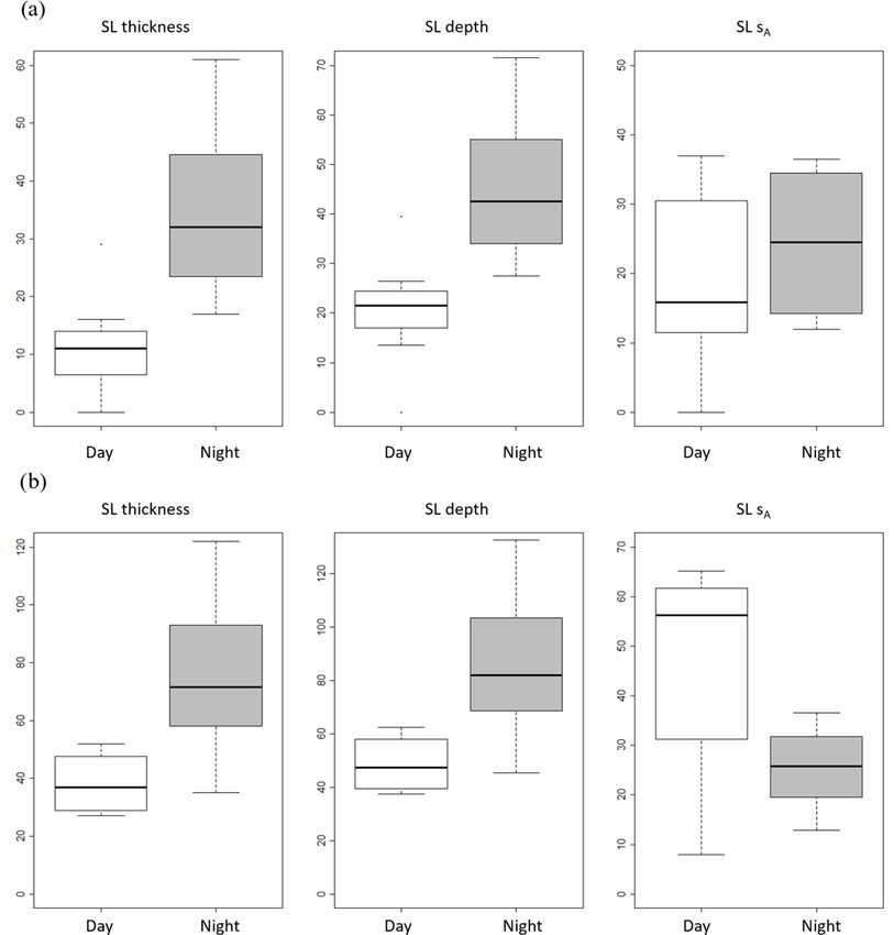
70               N. Diogoul et al.: Sound-scattering layers structure and its relationship to pelagic habitat characteristics

Figure 3. Discrimination of 36 CTD stations off the Senegalese coast: (1) two groups of stations were discriminated based on temperature
(temp), chlorophyll a (CHL), dissolved oxygen (oxy), and density (dens). (2) Principal component analysis of environmental parameters
for all 36 stations. (a) Eigenvalue diagram; (b) factor plane; (c) correlation circle. Group 1 represents stations located in the inshore area
(n = 18); Group 2 represents stations located in the offshore area (n = 18).

the coast (inshore area, from 13 to 61 m bottom depth, which             26.8 %. On axis 1 of the PCA plot, temperature was highly
encompassed the core of the upwelling (based on data for sea             correlated with density. On axis 2, temperature and DO were
surface temperature) (Fig. 1). Group 2 (G2) stations (n = 18)            opposed to CHL. The distribution of these variables is related
comprised seven stations along transect R1, six stations along           to the station groupings: G1 (inshore area) was characterized
transect R2, and five stations along transect R3. These sta-             by a dense and CHL-rich water mass, whereas G2 (offshore
tions were located furthest from shore (offshore area), from             area) was characterized by a warm and slightly oxygenated
41 to 205 m bottom depth, which corresponds to the outer                 surface water mass.
border of the upwelling zone. Considering the bathymetry,                   Satellite measurements of SST distributions of the study
we note an overlay of the two areas discriminated between                area indicated the same split of stations into two groups
41 and 61 m.                                                             (Fig. S6). The inshore area was characterized by low SST
   PCA identified the same two distinct water masses that                values (18–19 ◦ C), indicating a recently upwelled water
were clustered in HCA (Fig. 3). Axis 1 of the PCA eigenval-              mass, whereas an older water mass with higher SST values
ues explained 72.8 % of the inertia, whereas axis 2 explained            (20–21 ◦ C) prevailed offshore.

Ocean Sci., 16, 65–81, 2020                                                                              www.ocean-sci.net/16/65/2020/
N. Diogoul et al.: Sound-scattering layers structure and its relationship to pelagic habitat characteristics 71
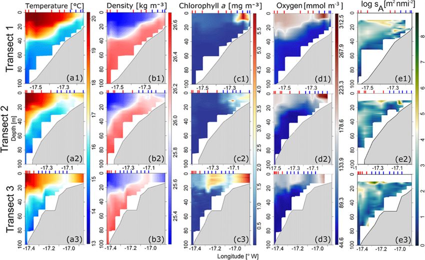
Figure 4. Contour plots of (a) temperature, (b) density, (c) chlorophyll-a concentration, (d) dissolved oxygen, and (e) square rooted nautical
area scattering coefficient (sA ) in the three transects (T1, T2, T3; see Fig. 1) with positions of vertical probe stations CTD in the inshore area
(vertical line in blue (G1)) and the offshore area (vertical line in red (G2)).
At transect T1, a marked frontal zone appeared isolat- concentration decreased from the surface to bottom in both
ing two water masses between the 20 and 40 m isobaths areas.
(Fig. 4a1), which separated warm surface waters from deep,
cold, upwelled water masses. At transects T2 and T3, the up- 3.2 Variability in vertical structure of SSLs
welling appeared as a cold-water tongue isolating a warm
water band at the coast (Fig. 4a2, a3). At T3, this cold-water 3.2.1 Spatial variability according to water mass
tongue was expanding toward the inshore area as well as characteristics
to the offshore area (Fig. 4a3). Surface water masses of the
inshore area were slightly denser than water masses in the Thickness and depth of the SSLs varied according to bottom
offshore area with approximately 26 and 25 kg m−3 , respec- depth in the inshore area and the offshore area. In the inshore
tively. For CHL, elevated concentrations were exclusively area, on the northern transect T1, no SSLs were observed at
observed in the inshore area at transects T1 and T2. CHL was coastal stations shallower than 29 m bottom depth (stations
significantly higher in the inshore area than the offshore area 1 and 2) (Fig. 5a). In offshore stations, starting at 41 m bot-
with concentrations of 3.0–5.0 mg m−3 in the inshore area to tom depth, the SSLs were observed in all stations and tran-
0.3–2.0 mg m−3 in the offshore area (Fig. 4c). At T3, the ele- sects (Fig. 5b), and their thickness and depth increased with
vated CHL concentrations were observed in both inshore and bottom depth. SSL thickness and SSL depth differed signif-
offshore areas close to the upwelling front. CHL was higher icantly between the inshore area and the offshore area: the
in the upper part of the water column (0–20 m), decreasing SSLs were thicker and deeper in the offshore area than in
with depth in both areas. Higher DO concentrations were the inshore area (Fig. 6) (p value = 0.001 for both thickness
observed towards both sides of the upwelling core. At T1, and depth). An increase of SSL was observed with increasing
the upwelling front was at the most coastal part, separating bottom depths in the inshore area and the offshore area. The
the inshore area from the less oxygenated offshore area with sA comparison between the inshore area and the offshore area
DO concentrations of 223–312 and 178–223 mmol m−3 , re- (Fig. 6) was not significantly different (p value = 0.833).
spectively. At T2 and T3, the core moved towards the off-
shore, separating the inshore area (DO concentrations of 3.2.2 Diel migration
178–223 mmol m−3 ), slightly more oxygenated than the off-
shore area (DO concentrations of 89–178 mmol m−3 ). DO The diel period had a significant effect on SSL thickness
(p value < 0.001) and SSL depth (p value < 0.001), which
www.ocean-sci.net/16/65/2020/ Ocean Sci., 16, 65–81, 202072 N. Diogoul et al.: Sound-scattering layers structure and its relationship to pelagic habitat characteristics
3.2.3 Vertical dimension of SSLs related to
physicochemical profile
In both areas, SSLs were partially or completely located
in areas of strong vertical gradients of temperature (ther-
mocline), density (pycnocline), and DO (oxycline) (Fig. 2).
When a strong temperature gradient was observed, usually
also associated with the vertical position of the oxycline and
a pycnocline, a peak of CHL was often observed and matched
with the volume backscattering strength (Sv ) peak (Fig. 2a).
This observation is well illustrated in CTD stations 12, 13,
16, and 25 (Fig. S8). In the inshore area the peak of CHL
concentration was always located above the SSLs (Fig. 2a),
whereas in the offshore area, the peak of CHL concentra-
tion was either above the SSLs or in the middle of the SSLs
(Fig. 2b). The thickest SSLs were observed in the offshore
area where temperature, density, and oxygen gradients were
strong.
3.2.4 Behavior of the SSLs relative to pelagic habitat
characteristics
In the inshore area (G1)
In the inshore area (G1), the ANCOVA model indicated a
strong effect of bottom depth and diel period on both SSL
thickness and depth. For SSL thickness, the model (Ta-
bles 1, S1 in the Supplement) explained 87 % of the vari-
ance (R 2 = 0.869, p value = 0.001). Bottom depth explained
56 % of SSL thickness, while the diel period effect accounted
Figure 5. Sound-scattering layer (SSL) mean depths (empty cir- for 31 %. The model of SSL depth (Tables 2, S2) was like
cle) according to their bottom depth, with their associated thickness those of SSL thickness; i.e., the model included bottom depth
(line, in meters) and SSL mean nautical area scattering coefficient
and diel period explaining 80 % of the variance (R 2 = 0.805,
(NASC or sA in m2 nmi−2 ), along transect 1 (south), transect 2
(intermediary), and transect 3 (north) during nighttime (black) and
p value = 0.001). Bottom depth showed the largest effect on
daytime (gray) sampling periods. SSLs explaining 51 % of SSL depth, while the diel period
effect was estimated at 30 %. For SSL acoustic density, i.e.,
log (sA ) (Tables 3, S3), the model explained 40 % of the vari-
were found higher during both the night in the inshore area ance (R 2 = 0.398, p value= 0.022), indicating a single effect
and the offshore area (Fig. 6). In the inshore area, during of bottom depth on log (sA ) (p value = 0.020). The bottom
daytime, the mean depth and thickness of SSL were 19 and depth was the only variable significant in the model and ex-
11 m, respectively, while during nighttime the mean depth plained 33 % of SSL acoustic density. Temperature was in-
and thickness were 46 and 35 m, respectively. In the offshore significant in the model.
area, SSLs were found at a mean depth and thickness of 49 The ANCOVA models to predict SSL thickness and SSL
and 38 m, respectively, during daytime, while during night- depth can be expressed as
time SSL depth and thickness were 86 and 75 m, respectively. SSLthickness = −11.865 + (0.916 × Bd ) + (11.492 × Dp ),
Mean sA (Fig. 6) of SSLs also varied between day and night
SSLdepth = −4.223 + (0.954 × Bd ) + (12.864 × Dp ),
but were not significantly different (p value = 0.890). In the
inshore area, the mean sA was 24 m2 nmi−2 during the day with Bd being bottom depth in meters and Dp being diel pe-
and 44 m2 nmi−2 during the night. In the offshore area, the riod at night.
mean sA was 46 m2 nmi−2 during daytime and 25 m2 nmi−2
during nighttime. Mean Sv distribution of SSLs (Fig. S7) also In the offshore area (G2)
showed a diel variation with mean Sv higher at night than
during the day. For offshore stations, the model showed a significant effect
of diel period, temperature, water density, and DO on both
thickness and depth of SSLs with similar results. Both mod-
els, SSL thickness (Tables 1, S1), and SSL depth (Tables 2,
Ocean Sci., 16, 65–81, 2020 www.ocean-sci.net/16/65/2020/N. Diogoul et al.: Sound-scattering layers structure and its relationship to pelagic habitat characteristics 73
Figure 6. Box plot (minimum, maximum, and median) of sound-scattering layers (SSLs) mean depth (m), thickness (m), and relative biomass
(sA in m2 nmi−2 ) grouped by diel period (day and night) for (a) inshore area and (b) offshore area over the Senegalese continental shelf.
S2) included bottom depth, diel period, temperature, density, 4 Discussion
and DO explaining 85 % of variance (R 2 = 0.855, p value
= 0.001). Bottom depth and diel period accounted for 28 % 4.1 Characterization of water masses along the Petite
and 28 %, respectively. Other significant variables were wa- Côte
ter temperature, density, and DO, which support 11 %, 10 %,
and 7 %, respectively. For SSL density or log(sA ) (Tables 3,
Upwelling is a key process for the functioning of the coastal
S3), none of the predictor variables had a significant effect.
ecosystem of Senegal and Mauritania (Capet et al., 2016;
The ANCOVA models to predict SSL thickness and SSL
Estrade et al., 2008; Rebert, 1983). By characterizing the
depth can be expressed as
physicochemical parameters of the Petite Côte, we were able
to discriminate two water masses: an inshore area and the
SSLthickness = 56030 + (0.21 × Bd ) + (27.35 × Dp ) offshore area, both of which could also be distinguished with
+ (−383.80 × T ) − (1898 × D) − (1.76 × O2 ), SST satellite data.
SSLdepth = 56040 + (0.21 × Bd ) + (27.35 × Dp ) Analyzing the spatial structure of SST helped to under-
stand the upwelling dynamics along the Petite Côte. The SST
+ (−383.80 × T ) − (1898 × D) − (1.76 × O2 ), pattern, measured at the time of our survey, was in line with
prior studies. During the upwelling season (in winter and
with Bd being bottom depth in meters, Dp being diel pe- late spring), a tongue of cold water over the shelf isolates
riod at night, T being water temperature in degrees Celcius a coastal band of warm water from the offshore area, and
(◦ C), D being water density (kg m−3 ), and O2 being oxygen there is a surface separation associated with the upwelling
(mmol m−3 ). source over the shelf and convergence nearshore. The spa-
www.ocean-sci.net/16/65/2020/ Ocean Sci., 16, 65–81, 202074 N. Diogoul et al.: Sound-scattering layers structure and its relationship to pelagic habitat characteristics
Table 1. Result of ANCOVA models between thickness of sound-scattering layers (SSLs) and environmental parameters (temperature,
density, dissolved oxygen, chlorophyll a, diel period, and bottom depth) in the inshore area (G1) and the offshore area (G2). G1: multiple
R 2 is 0.869, adjusted R 2 is 0.8515, and p value < 0.001; G2: multiple R 2 is 0.8557, adjusted R 2 is 0.7956, and p value < 0.001; significant
p values in bold.
Variable Significance Explained deviance ( %) Total explained
variance ( %)
Inshore Offshore Inshore Offshore Inshore Offshore
(G1) (G2) (G1) (G2) (G1) (G2)
Bottom depth 0.001 0.005 55.86 28.05
Diel period (night) 0.007 0.008 31.02 28.33
Temperature 0.007 11.29 86.9 85.57
Density 0.008 10.35
Oxygen 0.007 7.53
Table 2. Result of ANCOVA models between depth of sound-scattering layers (SSLs) and environmental parameters (temperature, density,
dissolved oxygen, chlorophyll a, diel period, and bottom depth) in the inshore area (G1) and the offshore area (G2). G1: multiple R 2 is
0.8056, adjusted R 2 is 0.7797, and p value is 0.001; G2: multiple R 2 is 0.8557, adjusted R 2 is 0.7956, and p value is 0.000; significant
p values in bold.
Variable Significance Explained deviance ( %) Total explained
variance ( %)
Inshore Offshore Inshore Offshore Inshore Offshore
(G1) (G2) (G1) (G2) (G1) (G2)
Bottom depth 0.001 0.005 55.86 28.05
Diel period (night) 0.021 0.008 31.02 28.33
Temperature 0.007 11.29 80.56 85.57
Density 0.008 10.35
Oxygen 0.007 7.53
tial difference of CHL concentration between the inshore crease due to biological remineralization of dissolved organic
area and the offshore area is the result of upwelled water matter (Emerson et al., 2008; Machu et al., 2019). These
carrying nutrients to the coast, which is separated by water low-oxygen bottom waters are transported to the inner shelf
mass fronts. Nutrient-rich water, supplied to the sunlit sur- during upwelling-favorable wind events. Moreover, temporal
face layer by wind-driven upwelling, stimulates the growth stability of the upwelling core is also noticeable over periods
of phytoplankton that ultimately fuel diverse and productive of several days to weeks, and export from the shelf to the
marine ecosystems (Jacox et al., 2018). There is a link be- open ocean is retarded (Capet et al., 2016). Thus, in such fa-
tween the accumulation of biological material and the loca- vorable conditions of continuous food supply, photosynthe-
tion of the coastal band of warm water. This coastal band sis may foster an enrichment of DO in the inshore. This is in
between coast and the upwelling core has been regarded to line with high CHL levels observed towards both sides of the
function as a retention area in which nutrient particles are upwelling core, particularly in the inshore area.
trapped (Demarcq and Faure, 2000; Roy, 1998). The nutrient
utilization is optimized by retentive physical mechanisms in 4.2 Spatial variation of the SSLs off the Petite Côte of
the coastal area, which enhances microbial remineralization Senegal
of particulate organic matter and zooplankton excretion and
then regenerates production through ammonium consump- We measured a longitudinal gradient of the thickness of the
tion (Auger et al., 2016). This causes an increase in primary SSLs over the continental shelf. The SSLs were concentrated
production and results in a surplus of phytoplankton biomass in a narrow band in the inshore area, whereas the SSLs were
in inshore areas. Low DO concentrations observed in the up- wider in the offshore zone. The absence or weakness of SSLs
welling core separating more oxygenated water masses have in the inshore area (in contrast to the more stratified water
been reported in previous studies (Capet et al., 2016; Teis- column in the offshore area) may have been due to turbu-
son, 1983) over the Petite Côte. Once a water mass becomes lence in the water column (Sengupta et al., 2017), coupled
isolated from the atmosphere, its oxygen content starts to de- with a well-mixed surface layer. In the inshore area, it is
Ocean Sci., 16, 65–81, 2020 www.ocean-sci.net/16/65/2020/N. Diogoul et al.: Sound-scattering layers structure and its relationship to pelagic habitat characteristics 75
likely that turbulence and the probable low residence time along our study area. Previous studies reported that DVM of
of marine pelagic organisms advected from outside this area plankton may increase coastal retention in the inshore area
and both inhibited SSL formation. Indeed, in such upwelling (Brochier et al., 2018; Mbaye et al., 2015; Rojas and Lan-
systems, in addition to the retention mechanism that has daeta, 2014). Diel variation was also observed for SSL acous-
been recognized by several authors (Arístegui et al., 2009; tic density, which showed opposite patterns in the two areas,
Capet et al., 2016; Mbaye et al., 2015; Roy, 1998), there i.e., higher up in the water column during night than day in
is also an offshore Ekman transport mechanism (Arístegui the inshore area and higher up during days than at night in
et al., 2009; Estrade et al., 2008) that contributes to cross- the offshore area. Tiedemann and Brehmer (2017) observed
shore exchanges. Otherwise, different animals can respond that all fish larvae in the offshore area, except Trachurus tra-
very differently to different physical forcing. Many authors churus, exhibited a DVM type II, and their observations are
have stressed that SSLs need stable hydrological conditions in accordance with the DVM pattern of SSL acoustic density
to form (Aoki and Inagaki, 1992; Baussant et al., 1992; Mar- reported in our study. Another possible explanation of this
chal et al., 1993). As an example, in Monterey Bay (Califor- observed diel variation is the horizontal migration. DHMs
nia), Urmy and Horne (2016) observed a decline in acous- are known as nocturnal horizontal migration of both plankton
tic backscatter intensity in the upper part of the water col- and consumers into shallow and inshore waters (Benoit-Bird
umn immediately following an upwelling event. In a more et al., 2001; Benoit-Bird and Au, 2006). DHMs have been
recent study, Benoit-Bird et al. (2019) found that when up- observed in marine copepods (Suh and Yu, 1996) which rep-
welling was strong both krill and anchovies were found in resent the main zooplankton group in the study area (Ndour
small, discrete aggregations, while during upwelling relax- et al., 2018; Rodrigues et al., 2017). It is hypothesized that
ation and reversals forage biomass was more diffusely dis- these inshore–offshore migrations are a strategy for avoiding
tributed. Therefore, we assume that the increase of SSL visual predators (White, 1998), and they result in increased
thickness with depth from inshore to offshore off Senegal is access to food resources relative to simple vertical migra-
caused by upwelled waters that disrupt the vertical stability tion (Benoit-Bird et al., 2008). Otherwise, DVM of marine
of the water column. Therefore, although the SSLs are first pelagic organisms may not be the only factor causing diel
constrained by the bottom depth (i.e., room available), we backscatter variations.
assume that the increase of SSL thickness with depth from
inshore to offshore off Senegal is caused by upwelled waters i. The acoustic target strength can be strongly dependent
that disrupt the vertical stability of the water column. on the aspect at which a target is insonified. Target
strengths of zooplankton and micronekton can vary by
4.3 Diel temporal variation of SSLs several orders of magnitude between extreme tilt angles,
i.e., horizontal vs. head up or head down (Benoit-Bird
In our study area, the diel period consistently exhibited pro- and Au, 2004; Yasuma et al., 2003). Target strength
nounced effects on SSL thickness and depth. Deeper night- is not independent of depth, as migrations through the
time SSLs have a greater thickness than daytime SSLs. The hydrostatic depth gradient can alter, e.g., swim blad-
diel difference in thickness and depth is due to the well- der volume (Fässler et al., 2009). This can bias target
known DVM patterns performed by many marine species. strengths, in particular near the resonance frequency,
DVM is a behavioral mechanism usually characterized by an leading to artificial increases of backscatter at a particu-
ascent during nighttime for feeding and a descent to avoid lar depth (Davison et al., 2015; Godø et al., 2009; Kloser
predation by visual predators during daytime known as type et al., 2002).
I (Bianchi et al., 2013; Haney, 1988; Lehodey et al., 2015).
ii. In the inshore area the CTD sampling was mainly
Some planktonic and micronektonic organisms have been re-
achieved during the daytime, which may have biased
ported to exhibit reverse DVM (type II), i.e., ascending in the
the observed DVM type I.
morning and descending in the evening or early night, which
is the opposite pattern generally observed with vertically mi- iii. Otherwise, plankton such as fish larvae are able to per-
grating animals (Cushing, 1951; Ohman et al., 1983). The form a DVM type II by ascending in the upper 10 m of
main SSL scatters much more strongly at 38 kHz than at 70 the water column at night, i.e., in the echo sounder off-
or 120 kHz (Fig. 2); the backscattering response is probably set.
dominated by animals with swim bladders such as fish lar-
vae and small fish (Simmonds and MacLennan, 2005a). In- 4.4 Effect of environmental parameters on SSLs
deed, the Petite Côte is a nursery area for fish and is the main
area in which juveniles of numerous species concentrate (Di- 4.4.1 SSLs related to physicochemical parameters in
ankha et al., 2018; Thiaw et al., 2017). Moreover, Tiedemann the vertical dimension
and Brehmer (2017) have reported fish larvae (Sardinella au-
rita, Engraulis encrasicolus, Trachurus trachurus, Trachurus Previous studies have shown that hydrographic structures of
trecae, Microchirus ocellatus, and Hygophum macrochi) all the water column influence SSL vertical structure (Balino
www.ocean-sci.net/16/65/2020/ Ocean Sci., 16, 65–81, 202076 N. Diogoul et al.: Sound-scattering layers structure and its relationship to pelagic habitat characteristics
Table 3. Result of ANCOVA models between sound-scattering-layer (SSL) density (log(sA )) and environmental parameters (temperature,
density, dissolved oxygen, chlorophyll a, diel period, and bottom depth) in the inshore area (G1) and the offshore area (G2). G1: multiple R 2
is 0.398, adjusted R 2 is 0.3178, and p value is 0.022; G2: multiple R 2 is 0.3448, adjusted R 2 is −0.01258, and p value is 0.490; significant
p values in bold.
Variable Significance Explained deviance ( %) Total explained
variance ( %)
Inshore Offshore Inshore Offshore Inshore Offshore
(G1) (G2) (G1) (G2) (G1) (G2)
Bottom depth 0.008 0.357 33.06 7.56
Temperature 0.119 0.273 6.73 5.17
Diel period (night) 0.007 0.546 7.22 39.8 34.48
Density 0.008 0.250 5.56
Oxygen 0.007 0.166 5.19
and Aksnes, 1993; Berge et al., 2014; Gausset and Turrel, by trophic relationships between phytoplankton, zooplank-
2001). In our case study the results show that vertical dis- ton, and micronekton. It is understood that zooplanktivorous
tribution of SSLs was linked to strong vertical gradients of micronekton migrates upward in the water column to forage
temperature, DO, and water density (Fig. 2). The peak of on mesozooplankton while the mesozooplankton is migrat-
Sv was sometimes very close to the strong gradient of wa- ing toward the surface to graze upon the phytoplankton. This
ter temperature, density, CHL, and DO (Fig. S8). The depth trophic relationship may explain the link in vertical position
of SSLs has been reported to be related to the thermocline of the SSLs with the phytoplankton peak reported in this
(Marchal et al., 1993; Yoon et al., 2007). In more stratified study.
areas, SSL vertical distribution was limited by a strong ther-
mocline and when thermocline was not well marked (low 4.4.2 Behavior of SSLs relative to pelagic habitat
gradient) SSLs occupied the entire water column (Lee et al., characteristics
2013). Olla and Davis (1990) and Rojas and Landaeta (2014)
suggested that the thermocline is a physical barrier that acts In the inshore area, where SSLs were sparsely present (or
above or below in the vertical distribution of some fish larvae, sometimes non-existent) bottom depth and diel period were
while other studies (Gray and Kingsford, 2003; Tiedemann the main environmental parameters influencing the vertical
and Brehmer, 2017) showed no effect of a thermocline on distribution (thickness and depth) of the SSLs. Bottom depth
vertical larval fish distributions. In this study, the SSL was has been shown to regulate the vertical distribution of SSLs
correlated to temperature in the offshore stratified area, but in the water column (Donaldson, 1967; Gausset and Turrel,
it did not act as a physical barrier limiting vertical distribu- 2001; Torgersen et al., 1997). In our study, all stations indi-
tion. Previous studies (Bertrand et al., 2010; Bianchi et al., cated a single SSL, while in deep water more thick and deep
2013; Netburn and Koslow, 2015) have suggested that verti- SSLs are often partitioned into multiple layers (Ariza et al.,
cal distributions of SSL organisms are limited by mid-water 2016; Balino and Aksnes, 1993; Cascão et al., 2017; Gaus-
DO concentrations which constrain SSL depth. These au- set and Turrel, 2001). Diel period is the second most impor-
thors found a relationship between SSL depths and hypoxia. tant parameter acting on SSL thickness and depth through
However, in our study, we found correlations between SSLs the DVM phenomenon. In well-mixed water masses, tem-
(depth, thickness) and DO as expected, but the vertical distri- perature, density, and oxygen had no effect on the SSLs. The
bution of SSLs was not constrained by DO. SSLs were also insignificant effect of temperature, oxygen, and water density
observed in some hypoxic stations (DO < 1.42 mL L−1 , i.e., on the SSLs in the inshore area is explained by the presence
63.42 mmol m−3 ); consequently, DO was not a limiting fac- of less marked and superficial clines because of the newly
tor for SSLs organisms. Fish larvae respond to oxygen gradi- upwelled water. As stated above, SSLs probably need stable
ents by moving upwards or laterally (Breitburg, 2002, 1994). conditions to occur.
Vertical movement of fish larvae may also be related to the In the offshore area, where vertical gradients were marked,
avoidance of predators, which are limited to well-oxygenated the main parameters structuring SSL thickness and depth
layers. The high phytoplankton concentration found in this were bottom depth and diel period but also water temper-
study, particularly in the inshore area, may be interpreted as ature, density, and DO. DVM behaviors are influenced by
a potential food source for fish larvae, which are able to per- environmental cues (e.g., light, nutrients, and temperature)
form DVM towards the surface. The vertical position of SSLs and predator–prey interactions (Clark and Levy, 1988; Lam-
compared to the CHL concentration peak can be explained pert, 1989). Relative changes in light intensity are identified
as the most important proximate stimuli driving DVM, in-
Ocean Sci., 16, 65–81, 2020 www.ocean-sci.net/16/65/2020/N. Diogoul et al.: Sound-scattering layers structure and its relationship to pelagic habitat characteristics 77
cluding the amplitude of the migration as well as the timing shown that the MLD can be tracked acoustically at high hor-
of the up- and downward movement (Meester, 2009). SSL izontal and vertical resolutions. The method was shown to be
vertical distribution is also known to be a function of temper- highly accurate when the MLD is well defined and biological
ature (Bertrand et al., 2010; Hazen and Johnston, 2010; Net- scattering does not dominate the acoustic returns. However,
burn and Koslow, 2015). Overnight, depths of the SSLs are in our study area, biological scattering dominated the acous-
strongly correlated to the depth of thermal and density gradi- tic records and due to the upwelling acoustic methods were
ents (Boersch-Supan et al., 2017; Cascão et al., 2017; Mar- not appropriate to determine MLD.
chal et al., 1993). In the offshore area, the results suggest that
DO also influences SSL depth and SSL thickness. In well-
oxygenated continental shelf waters, DO influences SSLs 5 Conclusions
but does not limit their vertical distribution. Some previous
work in French Polynesia (Bertrand et al., 2000), and in the Using our echogram vs. profile coupling approach, we were
southern California current ecosystem (Netburn and Koslow, able to examine fine-scale processes affecting SSL distribu-
2015), showed that the oxygen minimum zone (OMZ) acts tions. SSLs were influenced by turbulence level in the up-
like a barrier to SSLs in their vertical distribution. Bianchi et welling, which led to an offshore advection of SSL organ-
al. (2013) suggest that distribution of the open-ocean OMZ isms. SSL distributions were mainly structured by bottom
may modulate the depth of migration at the large scale so that depth, diel period, and the level of vertical stratification in
organisms within SSLs migrate to shallower waters in low- water column. SSL acoustic density variation suggested dif-
oxygen regions and to deeper waters in well-oxygenated wa- ferent diel migrations: a normal and reverse DVM, and/or a
ters. For both areas, CHL concentration was the only predic- DHM. Such an observation should be considered in mod-
tor that was not included in any of the final models. However, eling exercises to better understand DVM implications in
by coupling echogram and profile data (Fig. 2), we can argue ecosystem functioning. Further investigations should inte-
that a relation between CHL and SSLs exists even if it was grate small-scale turbulence measurements to better describe
not significant in the models, because CHL and SSL biomass the fine-scale spatiotemporal variability of SSLs and their re-
peaks matched, i.e., always located above or in the middle of lationship to the pelagic environment. Information on SSL
the SSLs. Moreover, a simple linear model between CHL and species composition and morphological characteristics will
SSL structure (depth and thickness) was significant in the in- provide an accurate description of their fine-scale relation-
shore area, suggesting that the effect of CHL on full models ships in the pelagic habitat.
was masked by autocorrelation between predictive variables.
Fish larvae vertical distributions have been related to the
distribution of their prey and predator, and it has been ar- Code availability. “Matecho” is an open-source tool available at
https://svn.mpl.ird.fr/echopen/MATECHO/ (last access: 15 Febru-
gued that the presence and position of the thermocline is an
ary 2019) (login: userecho, password: echopen). Other MATLAB
important feature in their vertical distribution (Haney, 1988;
codes used in this work are “Layer” and “ComparEchoProfil” and
Röpke, 1993). Other studies have shown that the thermocline are shared in the Supplement sections S1 and S2 of this paper. “Mat-
has only a limited role in the vertical distribution patterns echo” (Perrot et al., 2018) is an Open-Source Tool available at:
of fish larvae (Gray, 1996; Gray and Kingsford, 2003). In- https://svn.mpl.ird.fr/echopen/MATECHO/ (login: userecho, pass-
deed, in coastal areas, where the structure of the water col- word: echopen).
umn is less regular than in the open sea, the vertical distribu-
tion of fish larvae depends on the physics of the water col-
umn (Sánchez-Velasco et al., 2007) but also on the behav- Sample availability. The public cannot access our data because
ior of each species (Fortier and Harris, 1989). According to they belong to the partners who funded the oceanographic cruise.
Sánchez-Velasco et al. (2007), the vertical distribution of fish
larvae is closely related to the changes in the water column
structure, with most fish larvae concentrated in the stratum of Supplement. The supplement related to this article is available on-
maximum stability. Therefore, the vertical stratification level line at: https://doi.org/10.5194/os-16-65-2020-supplement.
in water column is strongly related to vertical distribution of
these organisms.
Furthermore, the vertical distribution of SSLs can be in- Author contributions. ND set the methodology, analyzed data, and
redacted the paper and the review. PB was cruise leader on the
fluenced by mixed layer depth (MLD). The MLD is one of
ECOAO sea survey, defined the sampling design, collected the data,
the primary factors affecting the vertical distribution of zoo-
defined the methodology, supervised the work and the review, and
plankton. Lee et al. (2018) have shown that the weighted took charge of the acquisition of the financial support for the project
mean depths of SSLs exhibit a strong linear relationship with leading to this publication. MT helped with data processing and
the MLD, meaning that the MLD could be a significant en- analyses, paper redaction, and the review. YP developed the “Mate-
vironmental factor controlling the habitat depth of marine cho” software tool and MATLAB code and contributed to the redac-
pelagic organisms. A recent study (Stranne et al., 2018) has tion and data collection. AS, AT, and SEA contributed to the PhD
www.ocean-sci.net/16/65/2020/ Ocean Sci., 16, 65–81, 202078 N. Diogoul et al.: Sound-scattering layers structure and its relationship to pelagic habitat characteristics
supervision of ND. AM and CM helped with statistical analyses and in the Canary Current upwelling, Prog. Oceanogr., 83, 33–48,
OS performed the early PCA on CTD data. https://doi.org/10.1016/j.pocean.2009.07.031, 2009.
Ariza, A., Landeira, J. M., Escánez, A., Wienerroither, R., Aguilar
de Soto, N., Røstad, A., Kaartvedt, S., and Hernández-León,
Competing interests. The authors declare that they have no conflict S.: Vertical distribution, composition and migratory patterns of
of interest. acoustic scattering layers in the Canary Islands, J. Mar. Syst.,
157, 82–91, https://doi.org/10.1016/j.jmarsys.2016.01.004,
2016.
Acknowledgements. Results of this paper were discussed during in- Auger, P.-A., Gorgues, T., Machu, E., Aumont, O., and Brehmer,
ternational conferences (ICAWA) in Dakar (2016) and in Mindelo P.: What drives the spatial variability of primary productiv-
(2017). We thank the participants for helpful comments made dur- ity and matter fluxes in the north-west African upwelling sys-
ing these conferences. We are thankful to the AWA project (Ecosys- tem? A modelling approach, Biogeosciences, 13, 6419–6440,
tem Approach to Management of Fisheries and Marine Environ- https://doi.org/10.5194/bg-13-6419-2016, 2016.
ment in West African Waters), funded by IRD and the BMBF (grant Balino, B. and Aksnes, D.: Winter distribution and migration of the
01DG12073E), and the PREFACE project (Enhancing Prediction sound scattering layers, zooplankton and micronekton in Mas-
of Tropical Atlantic Climate and its Impacts), and the TriAtlas fjorden, western Norway, Mar. Ecol. Prog. Ser., 102, 35–50,
project, as well as all IRD – ISRA/CRODT – Genavir staff for help- https://doi.org/10.3354/meps102035, 1993.
ing us at sea during the survey (https://doi.org/10.17600/13110030, Baussant, T., Ibanez, F., Dallot, S. and Etienne, M.: Diurnal
Brehmer, 2017). We thank Gildas Roudaut, Fabrice Roubaud, mesoscale patterns of 50-khz scattering layers across the lig-
François Baurand, and the US Imago (IRD) for data collec- urian sea front (NW mediterranean-sea), Oceanol. Acta, 15, 3–
tion aboard FRV Antea (IRD), the Gnavir crew of Antea, Do- 12, 1992.
minique Dagorne (IRD) curating satellite products, as well as the Belkin, I. M., Cornillon, P. C., and Sherman, K.: Fronts in
personal of ISRA/CRODT (Senegal), IRD DR-Ouest (France) and Large Marine Ecosystems, Prog. Oceanogr., 81, 223–236,
INRH (Morocco) for their administrative help during Ndague Dio- https://doi.org/10.1016/j.pocean.2009.04.015, 2009.
goul PhD stays in Morocco financed by OWSD (Organization Benoit-Bird, K., Au, W., E. Brainard, R., and Lammers, M.: Diel
for Women in Sciences for the Developing World). We thank horizontal migration of the Hawaiian mesopelagic boundary
Heino Fock (TI, Germany), as well as the anonymous referee, for community observed acoustically, Mar. Ecol. Prog. Ser., 217, 1–
their helpful comments on this paper, which significantly improved 14, https://doi.org/10.3354/meps217001, 2001.
the paper quality. Benoit-Bird, K. J. and Au, W. W. L.: Diel migration dynamics of an
island-associated sound-scattering layer, Deep-Sea Res. Pt. I, 51,
707–719, https://doi.org/10.1016/j.dsr.2004.01.004, 2004.
Benoit-Bird, K. J. and Au, W. W. L.: Extreme diel hor-
Financial support. This research has been supported by the IRD-
izontal migrations by a tropical nearshore resident mi-
BMBF (grant no. 01DG12073E).
cronekton community, Mar. Ecol. Prog. Ser., 319, 1–14,
https://doi.org/10.3354/meps319001, 2006.
Benoit-Bird, K. J., Zirbel, M. J., and McManus, M. A.: Diel varia-
Review statement. This paper was edited by Mario Hoppema and tion of zooplankton distributions in Hawaiian waters favors hori-
reviewed by Heino Fock and one anonymous referee. zontal diel migration by midwater micronekton, Mar. Ecol. Prog.
Ser., 367, 109–123, https://doi.org/10.3354/meps07571, 2008.
Benoit-Bird, K. J., Waluk, C. M., and Ryan, J. P.: Forage Species
Swarm in Response to Coastal Upwelling, Geophys. Res. Lett.,
References 46, 1537–1546, https://doi.org/10.1029/2018GL081603, 2019.
Berge, J., Cottier, F., Varpe, O., Renaud, P. E., Falk-Petersen,
Akaike, H.: A new look at the statistical model iden- S., Kwasniewski, S., Griffiths, C., Soreide, J. E., Johnsen, G.,
tification, IEEE T. Autom. Contr., 19, 716–723, Aubert, A., Bjaerke, O., Hovinen, J., Jung-Madsen, S., Tveit, M.,
https://doi.org/10.1109/TAC.1974.1100705, 1974. and Majaneva, S.: Arctic complexity: a case study on diel verti-
Akima, H., Gebhardt, A., Petzold, T., and Maechler, M.: akima: cal migration of zooplankton, J. Plankton Res., 36, 1279–1297,
Interpolation of Irregularly and Regularly Spaced Data, avail- https://doi.org/10.1093/plankt/fbu059, 2014.
able at: https://CRAN.R-project.org/package=akima (last access: Bertrand, A., Misselis, C., Josse, E., and Bach, P.: Caractéri-
8 July 2018), 2016. sation hydrologique et acoustique de l’habitat pélagique en
Anonymous: Rapport des travaux de recherches scientifiques à bord Polynésie française?: conséquences sur les distributions horizon-
du navire “ATLANTIDA” réalisés dans la Zone Economique Ex- tale et verticale des thonidés, in: Les espaces de l’Halieutique,
clusive (ZEE) du Sénégal (Décembre 2012), Rap. Scient., Atlant- Actes du quatrième Forum Halieumétrique, edited by: Gas-
Niro, Russie, 2013. cuel, D., Biseau, A., Bez, N., and Chavance, P., 55–74, Paris,
Aoki, I. and Inagaki, T.: Acoustic observations of fish schools and available at: http://horizon.documentation.ird.fr/exl-doc/pleins_
scattering layers in a Kuroshio warm-core ring and its environs, textes/divers09-03/010024490.pdf, (last access: 20 Novem-
Fish. Oceanogr., 1, 137–142, 1992. ber 2019), 2000.
Arístegui, J., Barton, E. D., Álvarez-Salgado, X. A., Santos, A. M. Bertrand, A., Ballón, M., and Chaigneau, A.: Acoustic Ob-
P., Figueiras, F. G., Kifani, S., Hernández-León, S., Mason, E., servation of Living Organisms Reveals the Upper Limit
Machú, E., and Demarcq, H.: Sub-regional ecosystem variability
Ocean Sci., 16, 65–81, 2020 www.ocean-sci.net/16/65/2020/You can also read