Depth Uncertainty in Neural Networks
←
→
Page content transcription
If your browser does not render page correctly, please read the page content below
Depth Uncertainty in Neural Networks

                                                             Javier Antorán∗                    James Urquhart Allingham∗
                                                          University of Cambridge                 University of Cambridge
                                                            ja666@cam.ac.uk                          jua23@cam.ac.uk
arXiv:2006.08437v1 [stat.ML] 15 Jun 2020

                                                                          José Miguel Hernández-Lobato
                                                                               University of Cambridge
                                                                                 Microsoft Research
                                                                              The Alan Turing Institute
                                                                                 jmh233@cam.ac.uk

                                                                                       Abstract
                                                       Existing methods for estimating uncertainty in deep learning tend to require
                                                       multiple forward passes, making them unsuitable for applications where
                                                       computational resources are limited. To solve this, we perform probabilistic
                                                       reasoning over the depth of neural networks. Different depths correspond to
                                                       subnetworks which share weights and whose predictions are combined via
                                                       marginalisation, yielding model uncertainty. By exploiting the sequential
                                                       structure of feed-forward networks, we are able to both evaluate our training
                                                       objective and make predictions with a single forward pass. We validate
                                                       our approach on real-world regression and image classification tasks. Our
                                                       approach provides uncertainty calibration, robustness to dataset shift, and
                                                       accuracies competitive with more computationally expensive baselines.

                                           1       Introduction
                                           Despite the widespread adoption of deep learning, building models that provide robust
                                           uncertainty estimates remains a challenge. This is especially important for real-world
                                           applications, where we cannot expect the distribution of observations to be the same as that
                                           of the training data. Deep models tend to be pathologically overconfident, even when their
                                           predictions are incorrect (Amodei et al., 2016; Nguyen et al., 2015). If AI systems would
                                           reliably identify cases in which they expect to underperform, and request human intervention,
                                           they could more safely be deployed in medical scenarios (Filos et al., 2019) or self-driving
                                           vehicles (Fridman et al., 2019), for example.
                                           In response, a rapidly growing subfield has emerged seeking to build uncertainty aware
                                           neural networks (Hernández-Lobato and Adams, 2015; Gal and Ghahramani, 2016; Laksh-
                                           minarayanan et al., 2017). Regrettably, these methods rarely make the leap from research
                                           to production due to a series of shortcomings. 1) Implementation Complexity: they can be
                                           technically complicated and sensitive to hyperparameter choice. 2) Computational cost: they
                                           can take orders of magnitude longer to converge than regular networks or require training
                                           multiple networks. At test time, averaging the predictions from multiple models is often
                                           required. 3) Weak performance: they rely on crude approximations to achieve scalability,
                                           often resulting in limited or unreliable uncertainty estimates (Foong et al., 2019a).
                                           In this work, we introduce Depth Uncertainty Networks (DUNs), a probabilistic model that
                                           treats the depth of a Neural Network (NN) as a random variable over which to perform
                                               ∗
                                                   equal contribution

                                           Preprint. Under review.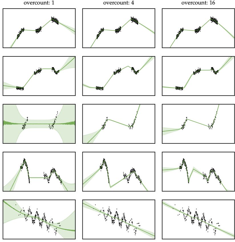
x   f0   ŷ0
x   f0   f1    ŷ1
x   f0   f1    f2    ŷ2
x   f0   f1    f2    f3    ŷ3
x   f0   f1    f2    f3    f4    ŷ4

Figure 1: A DUN is composed of subnetworks of increasing depth (left, colors denote
layers with shared parameters). These correspond to increasingly complex functions (centre,
colors denote depth at which predictions are made). Marginalising over depth yields model
uncertainty through disagreement of these functions (right, error bars denote 1 std. dev.).

inference. In contrast to more typical weight-space approaches for Bayesian inference in NNs,
ours reflects a lack of knowledge about how deep our network should be. We treat network
weights as learnable hyperparameters. In DUNs, marginalising over depth is equivalent to
performing Bayesian Model Averaging (BMA) over an ensemble of progressively deeper NNs.
As shown in Figure 1, DUNs exploit the overparametrisation of a single deep network to
generate diverse explanations of the data. The key advantages of DUNs are:

     1. Implementation simplicity: requiring only minor additions to vanilla deep learning
        code, and no changes to the hyperparameters or training regime.
     2. Cheap deployment: computing exact predictive posteriors with a single forward pass.
     3. Calibrated uncertainty: our experiments show that DUNs are competitive with strong
        baselines in terms of predictive performance, Out-of-distribution (OOD) detection
        and robustness to corruptions.

2   Related Work
Traditionally, Bayesians tackle overconfidence in deep networks by treating their weights
as random variables. Through marginalisation, uncertainty in weight-space is translated to
predictions. Alas, the weight posterior in Bayesian Neural Networks (BNNs) is intractable.
Hamiltonian Monte Carlo (Neal, 1995) remains the gold standard for inference in BNNs but
is limited in scalability. The Laplace approximation (MacKay, 1992; Ritter et al., 2018),
Variational Inference (VI) (Hinton and van Camp, 1993; Graves, 2011; Blundell et al., 2015)
and expectation propagation (Hernández-Lobato and Adams, 2015) have all been proposed
as alternatives. More recent methods are scalable to large models (Khan et al., 2018; Osawa
et al., 2019; Dusenberry et al., 2020). Gal and Ghahramani (2016) re-interpret dropout as
VI, dubbing it MC Dropout. Other stochastic regularisation techniques can also be viewed in
this light (Gal, 2016; Kingma et al., 2015; Teye et al., 2018). These can be seamlessly applied
to vanilla networks. Regrettably, most of the above approaches rely on factorised, often
Gaussian, approximations resulting in pathological overconfidence (Foong et al., 2019a).
It is not clear how to place reasonable priors over network weights (Wenzel et al., 2020). DUNs
avoid this issue by targeting depth. BNN inference can also be performed directly in function
space (Sun et al., 2019; Hafner et al., 2018; Ma et al., 2019; Wang et al., 2019). However,
this requires crude approximations to the KL divergence between stochastic processes. The
equivalence between infinitely wide NNs and Gaussian processes (GPs) (Neal, 1995; Matthews
et al., 2018; Garriga-Alonso et al., 2019) can be used to perform exact inference in BNNs.
Unfortunately, exact GP inference scales poorly in dataset size.
Deep ensembles is a non-Bayesian method for uncertainty estimation in NNs that trains
multiple independent networks and aggregates their predictions (Lakshminarayanan et al.,
2017). Ensembling provides very strong results but is limited by its computational cost.
Huang et al. (2017), Garipov et al. (2018), and Maddox et al. (2019) reduce the cost of
training an ensemble by leveraging different weight configurations found in a single SGD
trajectory. However, this comes at the cost of reduced predictive performance (Ashukha
et al., 2020). Similarly to deep ensembles, DUNs combine the predictions from a set of deep
models. However, this set stems from treating depth as a random variable. Unlike ensembles,

                                              2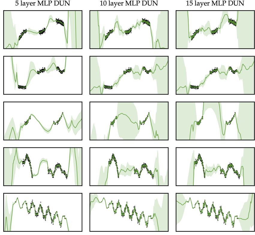
x     f0
       (n)
       x                                 f1
               β                                  f2
                                                            f3                                        fD+1   ŷi

 θ     (n)
       y       d                                                        f4

           N                                                                               fD

Figure 2: Left: graphical model under consideration. Right: computational model. Each
layer’s activations are passed through the output block, producing per-depth predictions.

BMA assumes the existence of a single correct model (Minka, 2000). In DUNs, uncertainty
arises due to a lack of knowledge about how deep the correct model is. It is worth noting
that deep ensembles can also be interpreted as approximate BMA (Wilson, 2020).
All of the above methods, except DUNs, require multiple forward passes to produce uncer-
tainty estimates. This is problematic in low-latency settings or those in which computational
resources are limited. Postels et al. (2019) use error propagation to approximate the dropout
predictive posterior with a single forward pass. Although efficient, this approach shares
pathologies with MC Dropout. van Amersfoort et al. (2020) combine deep RBF networks
with a Jacobian regularisation term to deterministically detect OOD points. Nalisnick et al.
(2019c) and Meinke and Hein (2020) use generative models to detect OOD data without
multiple predictor evaluations. Unfortunately, deep generative models can be unreliable for
OOD detection (Nalisnick et al., 2019b) and simpler alternatives might struggle to scale.
There is a rich literature on probabilistic inference for NN structure selection, starting with
the Automatic Relevance Detection prior (MacKay et al., 1994). Since then, a number of
approaches have been introduced (Ghosh et al., 2019; Dikov and Bayer, 2019; Lawrence, 2002).
Perhaps the closest to our work is the Automatic Depth Determination prior (Nalisnick et al.,
2019a). Huang et al. (2016) stochastically drop layers as a ResNet training regularisation
approach. Conversely, DUNs perform marginalisation over architectures, translating depth
uncertainty into uncertainty over a broad range of functional complexities.

3     Depth Uncertainty Networks

Consider a dataset D = {x(n) , y(n) }N n=1 and a neural network composed of an input block
f0 (·), D intermediate blocks {fi (·)}D
                                      i=1 , and an output block fD+1 (·). Each block is a group
of one or more stacked linear and non-linear operations. The activations at depth i ∈ [0, D],
ai , are obtained recursively as ai = fi (ai−1 ), a0 = f0 (x).
A forward pass through the network is an iterative process, where each successive block fi (·)
refines the previous block’s activation. Predictions can be made at each step of this procedure
by applying the output block to each intermediate block’s activations: ŷi = fD+1 (ai ). This
computational model is displayed in Figure 2. It can be implemented by changing 8 lines in
a vanilla PyTorch NN, as shown in Appendix H. Recall, from Figure 1, that we can leverage
the disagreement among intermediate blocks’ predictions to quantify model uncertainty.

3.1   Probabilistic Model: Depth as a Random Variable

We place a categorical prior over network depth pβ (d) = Cat(d|{βi }D
                                                                    i=0 ). Referring to net-
work weights as θ, we parametrise the likelihood for each depth using the corresponding
subnetwork’s output: p(y|x, d=i; θ) = p(y|fD+1 (ai ; θ)). A graphical model is shown in
Figure 2. For a given weight configuration, the likelihood for every depth, and thus our
model’s Marginal Log Likelihood (MLL):
                                       D                   N
                                                                                                !
                                       X                   Y
                   log p(D; θ) = log          pβ (d=i) ·         p(y   (n)
                                                                             |x   (n)
                                                                                        , d=i; θ) ,                (1)
                                       i=0                 n=1

                                                       3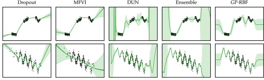
can be obtained with a single forward pass over the training set by exploiting the sequential
nature of feed-forward NNs. The posterior over depth, p(d|D; θ)=p(D|d; θ)pβ (d)/p(D; θ) is
a categorical distribution that tells us about how well each subnetwork explains the data.
A key advantage of deep neural networks lies in their capacity for automatic feature extraction
and representation learning. For instance, Zeiler and Fergus (2014) demonstrate that CNNs
detect successively more abstract features in deeper layers. Similarly, Frosst et al. (2019) find
that maximising the entanglement of different class representations in intermediate layers
yields better generalisation. Given these results, using all of our network’s intermediate
blocks for prediction might be suboptimal. Instead, we infer whether each block should be
used to learn representations or perform predictions, which we can leverage for ensembling, by
treating network depth as a random variable. As shown in Figure 3, subnetworks too shallow
to explain the data are assigned low posterior probability; they perform feature extraction.

3.2   Inference in DUNs
We consider learning network weights by directly maximising (1) with respect to θ, using
backpropagation and the log-sum-exp trick. In Appendix B, we show that the gradients of
(1) reaching each subnetwork are weighted by the corresponding depth’s posterior mass. This
leads to local optima where all but one subnetworks’ gradients vanish. The posterior collapses
to a delta function over an arbitrary depth, leaving us with a deterministic NN. When working
with large datasets, one might indeed expect the true posterior over depth to be a delta.
However, because modern NNs are underspecified even for large datasets, multiple depths
should be able to explain the data simultaneously (shown in Figure 3 and Appendix B).
We can avoid the above pathology by decoupling the optimisation of network weights θ from
the posterior distribution. In latent variable models, the Expectation Maximisation (EM) al-
gorithm (Bishop, 2006) allows us to optimise the MLL by iteratively computing p(d|D; θ) and
then updating θ. We propose to use stochastic gradient variational inference as an alternative
more amenable to NN optimisation. We introduce a surrogate categorical distribution over
depth qα (d) = Cat(d|{αi }Di=0 ). In Appendix A, we derive the following lower bound on (1):
                                 N
                                 X            h                        i
       log p(D; θ) ≥ L(α, θ) =         Eqα (d) log p(y(n) |x(n) , d; θ) − KL(qα (d) k pβ (d)).   (2)
                                 n=1

This Evidence Lower BOund (ELBO) allows us to optimise the variational parameters α and
network weights θ simultaneously using gradients. Because both our variational and true
posteriors are categorical, (2) is convex with respect to α. At the optima, qα (d) = p(d|D; θ)
and the bound is tight. Thus, we perform exact rather than approximate inference.
Eqα (d) [log p(y|x, d; θ)] can be computed from the activations at every depth. Consequently,
both terms in (2) can be evaluated exactly, with only a single forward pass. This removes
the need for high variance Monte Carlo gradient estimators, often required by VI methods
for NNs. When using mini-batches of size B, we stochastically estimate the ELBO in (2) as
                              B D                                  D
                          N XX                                X              αi
              L(α, θ) ≈              log p(y |x , d=i; θ) · αi −
                                            (n) (n)
                                                                        αi log      .    (3)
                          B n=1 i=0                               i=0
                                                                               βi
Predictions for new data x∗ are made by marginalising depth with the variational posterior:
                                             D
                                             X
                        p(y∗ |x∗ , D; θ) =         p(y∗ |x∗ , d=i; θ)qα (d=i).                   (4)
                                             i=0

4     Experiments
First, we compare the MLL and VI training approaches for DUNs. We then evaluate DUNs on
toy-regression, real-world regression, and image classification tasks. As baselines, we provide
results for vanilla NNs (denoted as ‘SGD’), MC Dropout (Gal and Ghahramani, 2016), and
deep ensembles (Lakshminarayanan et al., 2017), arguably the strongest approach for uncer-
tainty estimation in deep learning (Ashukha et al., 2020; Snoek et al., 2019). For regression

                                                    4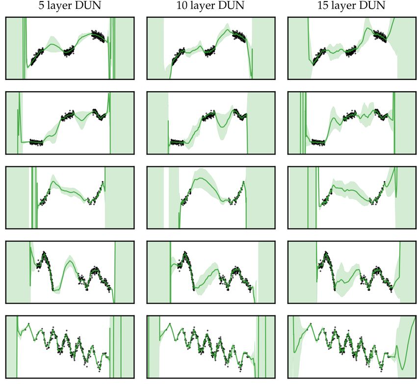
MLL Objective VI Objective
1500
MLL
1000
ELBO
nats
500
0
−500
probabilities 100 p ( d =0)
p ( d =1)
10−1
p ( d =2)
10−2 p ( d =3)
p ( d =4)
10−3 p ( d =5)
0 1000 2000 3000 4000 0 1000 2000 3000 4000
epochs epochs
Figure 3: Top row: progression of MLL and ELBO during training. Bottom: progression of
all six depth posterior probabilities. The left column corresponds to optimising the MLL
directly and the right to VI. For the latter, variational posterior probabilities q(d) are shown.
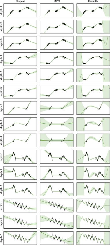
Figure 4: Top row: toy dataset from Izmailov et al. (2019). Bottom: Wiggle dataset. Black
dots denote data points. Error bars represent standard deviation among mean predictions.
tasks, we also include Gaussian Mean Field VI (MFVI) (Blundell et al., 2015) with the local
reparametrisation trick (Kingma et al., 2015). We study all methods in terms of accuracy, un-
certainty quantification, and robustness to corrupted or OOD data. We place a uniform prior
over DUN depth. See Appendix C, Appendix D, and Appendix E for detailed descriptions of
the techniques we use to compute, and evaluate uncertainty estimates, and our experimental
setup, respectively. Code is available at https://github.com/cambridge-mlg/DUN.
4.1 Comparing MLL and VI training
Figure 3 compares the optimisation of a 5 hidden layer fully connected DUN on the concrete
dataset using estimates of the MLL (1) and ELBO (3). The former approach converges to a
local optima where all but one depth’s probabilities go to 0. With VI, the surrogate posterior
converges slower than the network weights. This allows θ to reach a configuration where
multiple depths can be used for prediction. Towards the end of training, the variational gap
vanishes. The surrogate distribution approaches the true posterior without collapsing to a
delta. The MLL values obtained with VI are larger than those obtained with (1), i.e. our
proposed approach finds better explanations for the data. In Appendix B, we optimise (1)
after reaching a local optima with VI (3). This does not cause posterior collapse, showing
that MLL optimisation’s poor performance is due to a propensity for poor local optima.
4.2 Toy Datasets
We consider two synthetic 1D datasets, shown in Figure 4. We use 3 hidden layer, 100
hidden unit, fully connected networks with residual connections for our baselines. DUNs
use the same architecture but with 15 hidden layers. GPs use the RBF kernel. We found
these configurations to work well empirically. In Appendix F.1, we perform experiments with
5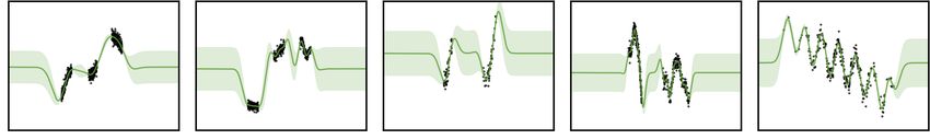
rank ↓ boston concrete energy kin8nm naval power protein wine yacht
−0.9
5 −2.25 −2.8 −1.0
1.25 5.5 −2.6
4 −2.50 −2.9 −1.0
1.20 −2.7 −1.0 −1.5
5.0 −2.7
−3.0
LL
3 −2.75
1.15
−3.1 −1.5 4.5 −1.1 −2.0
−2.8 −2.8
2 −3.00 1.10
−3.2 4.0
−3.25 −2.0 1.05 −2.9 −2.5
1 −1.2
−3.3 −2.9
3.5
4.0 1.75 0.085 0.006
5 6.0 4.5
4.25 0.68 2.5
1.50
4 3.5 5.5 0.080
RMSE
0.004 4.00 0.66 2.0
1.25 4.0
3 0.075
3.0 5.0 1.00 3.75 0.64 1.5
2 0.002
0.75 0.070 3.50 3.5 1.0
4.5 0.62
1 2.5
0.50
0.065 3.25 0.60 0.5
0.14 0.08 0.30 0.10
5 0.05 0.10
0.25 0.4
0.12 0.06 0.25
0.08
4 0.06 0.20 0.04 0.08
0.10 0.20 0.3
TCE
3 0.15 0.04 0.06
0.08 0.15 0.03 0.06
0.04 0.2
2 0.06 0.10 0.04
0.10 0.02 0.04
0.02 0.1
0.04 0.05
1 0.05 0.02
0.02 0.02
0.01
5 0.20
0.06 0.06 0.15 0.04
0.100
0.03 0.15
batch time
4 0.15
0.2 0.075 0.03
0.04 0.04 0.10
0.02 0.10
3 0.10
0.050 0.02
0.1
0.01 0.02 0.02 0.05 0.05
2 0.05 0.025 0.01
1 0.00 0.00 0.00 0.00 0.00 0.00 0.0 0.000 0.00
DUN Dropout Ensemble MFVI SGD
Figure 5: Quartiles for results on UCI regression datasets across standard splits. Average
ranks are computed across datasets. For LL, higher is better. Otherwise, lower is better.
different toy datasets, architectures and hyperparameters. DUNs’ performance increases
with depth but often 5 layers are sufficient to produce reasonable uncertainty estimates.
The first dataset, which is taken from Izmailov et al. (2019), contains three disjoint clusters
of data. Both MFVI and Dropout present error bars that are similar in the data dense and
in-between regions. MFVI underfits slightly, not capturing smoothness in the data. DUNs
perform most similarly to Ensembles. They are both able to fit the data well and express in-
between uncertainty. Their error bars become large very quickly in the extrapolation regime.
Our second dataset consists of 300 samples from y= sin(πx)+0.2 cos(4πx)−0.3x+, where
∼ N (0, 0.25) and x ∼ N (5, 2.5). We dub it “Wiggle”. Dropout struggles to fit this
faster varying function outside of the data-dense regions. MFVI fails completely. DUNs and
Ensembles both fit the data well and provide error bars that grow as the data becomes sparse.
4.3 Tabular Regression
We evaluate all methods on UCI regression datasets using standard (Hernández-Lobato and
Adams, 2015) and gap splits (Foong et al., 2019b). We also use the large-scale non-stationary
flight delay dataset, preprocessed by Hensman et al. (2013). Following Deisenroth and Ng
(2015), we train on the first 2M data points and test on the subsequent 100k. We select all
hyperparameters, including NN depth, using Bayesian optimisation with HyperBand (Falkner
et al., 2018). See Appendix E.2 for details. We evaluate methods with Root Mean Squared
Error (RMSE), Log Likelihood (LL) and Tail Calibration Error (TCE). The latter measures
the calibration of the 10% and 90% confidence intervals, and is described in Appendix D.
UCI standard split results are found in Figure 5. For each dataset and metric, we rank
methods from 1 to 5 based on mean performance. We report mean ranks and standard
deviations. Dropout obtains the best mean rank in terms of RMSE, followed closely
by Ensembles. DUNs are third, significantly ahead of MFVI and SGD. Even so, DUNs
outperform Dropout and Ensembles in terms of TCE, i.e. DUNs more reliably assign large
6
Table 1: Results obtained on the flights dataset (2M). Mean and standard deviation values
are computed across 5 independent training runs.
           Metric      DUN         Dropout         Ensemble     MFVI          SGD
           LL        −4.95±0.01   −4.95±0.02    −4.95±0.01    −5.02±0.05   −4.97±0.01
           RMSE      34.69±0.28   34.28±0.11    34.32±0.13    36.72±1.84   34.61±0.19
           TCE        .087±.009    .096±.017     .090±.008    .068±.014     .084±.010
           Time       .026±.001    .016±.001     .031±.001     .547±.003   .002±.000

error bars to points on which they make incorrect predictions. Consequently, in terms of
LL, a metric which considers both uncertainty and accuracy, DUNs perform competitively
(the LL rank distributions for all three methods overlap almost completely). MFVI provides
the best calibrated uncertainty estimates. Despite this, its mean predictions are inaccurate,
as evidenced by it being last in terms of RMSE. This leads to MFVI’s LL rank only being
better than SGD’s. Results for gap splits, designed to evaluate methods’ capacity to express
in-between uncertainty, are given in Appendix F.2. Here, DUNs outperform Dropout in
terms of LL rank. However, they are both outperformed by MFVI and ensembles.
The flights dataset is known for strong covariate shift between its train and test sets, which
are sampled from contiguous time periods. LL values are strongly dependent on calibrated
uncertainty. As shown in Table 1, DUNs’ RMSE is similar to that of SGD, with Dropout
and Ensembles performing best. Again, DUNs present superior uncertainty calibration. This
allows them to achieve the best LL, tied with Ensembles and Dropout. We speculate that
DUNs’ calibration stems from being able to perform exact inference, albeit in depth space.
In terms of prediction time, DUNs clearly outrank Dropout, Ensembles, and MFVI on UCI.
Due to depth, or maximum depth D for DUNs, being chosen with Bayesian optimisation,
methods’ batch times vary across datasets. DUNs are often deeper because the quality of
their uncertainty estimates improves with additional explanations of the data. As a result,
SGD clearly outranks DUNs. On flights, increased depth causes DUNs’ prediction time to
lie in between Dropout’s and Ensembles’.

4.4      Image Classification

We train ResNet-50 (He et al., 2016) using all methods under consideration. This model
is composed of an input convolutional block, 16 residual blocks and a linear layer. For
DUNs, our prior over depth is uniform over the first 13 residual blocks. The last 3 residual
blocks and linear layer form the output block, providing the flexibility to make predictions
from activations at multiple resolutions. We use 1 × 1 convolutions to adapt the number
of channels between earlier blocks and the output block. We use default PyTorch training
hyperparameters2 for all methods. We set per-dataset LR schedules. We use 5 element
ensembles, as suggested by Snoek et al. (2019), and 10 dropout samples. Figure 6 contains
results for all experiments described below. Mean values and standard deviations are
computed across 5 independent training runs. Full details are given in Appendix E.3.

Rotated MNIST Following Snoek et al. (2019), we train all methods on MNIST and
evaluate their predictive distributions on increasingly rotated digits. Although all methods
perform well on the original test-set, their accuracy degrades quickly for rotations larger than
30°. Here, DUNs differentiate themselves by being the least overconfident. We hypothesize
that predictions based on features at diverse resolutions allow for increased disagreement.

Corrupted CIFAR Again following Snoek et al. (2019), we train models on CIFAR10
and evaluate them on data subject to 16 different corruptions with 5 levels of intensity
each (Hendrycks and Dietterich, 2019). Here, Ensembles significantly outperform all single
network methods in terms of error and LL at all corruption levels. DUNs perform similarly
to SGD and Dropout on the uncorrupted data. Despite only requiring a single forward pass
for predictions, LL values reveal DUNs to be second most robust to corruption.
   2
       https://github.com/pytorch/examples/blob/master/imagenet/main.py

                                               7
Rotated MNIST Corruption Robustness
0.4
error
0.5
0.2
0.0
0
−0.5
−2
−1.0
LL
−4 −1.5
−2.0
−6
−2.5
0 30 60 90 120 150 180 0 1 2 3 4 5
rotation (◦ ) corruption
OOD Rejection Compute Time
1.0 15 20
−1.6 10
7
5
0.8 −1.8
accuracy
3
DUN
−2.0
LL
2 Ensemble
0.6
−2.2 10 15 20 Dropout
5 7
23 SGD
0.4 −2.4 1 DUN (exact)
0 25 50 75 100 0.0 0.5 1.0 1.5 2.0 2.5 3.0
% rejected time (s)
Figure 6: Top left: error and LL for MNIST at varying degrees of rotation. Top right:
error and LL for CIFAR10 at varying corruption severities. Bottom left: CIFAR10-SVHN
rejection-classification plot. The black line denotes the theoretical maximum performance; all
in-distribution samples are correctly classified and OOD samples are rejected first. Bottom
right: Pareto frontiers showing LL for corrupted CIFAR10 (severity 5) vs batch prediction
time. Batch size is 256, split over 2 Nvidia P100 GPUs. Annotations show ensemble elements
and Dropout samples. Note that a single element ensemble is equivalent to SGD.
OOD Rejection We simulate a realistic OOD rejection scenario (Filos et al., 2019) by
jointly evaluating our models on an in-distribution and an OOD test set. We allow our
methods to reject increasing proportions of the data based on predictive entropy before
classifying the rest. All predictions on OOD samples are treated as incorrect. Following
Nalisnick et al. (2019b), we use CIFAR10 and SVHN as in and out of distribution datasets.
Ensembles perform best. In their standard configuration, DUNs show underconfidence. They
are incapable of separating very uncertain in-distribution inputs from OOD points. We re-run
DUNs using the exact posterior over depth p(d|D; θ) in (4), instead of qα (d). The exact
posterior is computed while setting batch-norm to test mode. This resolves underconfidence,
outperforming dropout and coming within error of ensembles. We don’t find exact posteriors
to improve performance in any other experiments. Hence we abstain from using them, as
they require an additional evaluation of the train set.
Compute Time We compare methods’ performance on corrupted CIFAR10 (severity 5)
as a function of computational budget. The LL obtained by a DUN matches that of a ∼1.8
element ensemble. A single DUN forward pass is ∼1.02 times slower than a vanilla network’s.
On average, DUNs’ computational budget matches that of ∼0.47 ensemble elements or ∼0.94
dropout samples. These values are smaller than one due to overhead such as ensemble element
loading. Thus, making predictions with DUNs is 10× faster than with five element ensembles.
5 Discussion and Future Work
We have re-cast NN depth as a random variable, as opposed to a fixed parameter. This
treatment allows us to optimise weights as model hyperparameters, preserving much of the
8simplicity of non-Bayesian NNs. Critically, both the model evidence and predictive posterior
for DUNs can be evaluated with a single forward pass. Our experiments show that DUNs
produce well calibrated uncertainty estimates, performing well relative to their computational
budget on uncertainty-aware tasks. They scale to modern architectures and large datasets.
In DUNs, network weights have dual roles: fitting the data well and expressing diverse
predictive functions at each depth. In future work, we would like to develop optimisation
schemes that better ensure both roles are fulfilled. We would also like to investigate the
effects of DUN depth on uncertainty estimation, allowing for more principled model selection.
Broader Impact
We have introduced a general method for training neural networks to capture model uncer-
tainty. These models are fairly flexible and can be applied to a large number of applications,
including potentially malicious ones. Perhaps, our method could have the largest impact on
critical decision making applications, where reliable uncertainty estimates are as important
as the predictions themselves. Financial default prediction and medical diagnosis would be
examples of these.
We hope that this work will contribute to increased usage of uncertainty aware deep learning
methods in production. DUNs are trained with default hyperparameters and easy to make
converge to reasonable solutions. The computational cost of inference in DUNs is similar to
that of vanilla NNs. This makes DUNs especially well suited for applications with real-time
requirements or low computational resources, such as self driving cars or sensor fusion on
embedded devices. More generally, DUNs make leveraging uncertainty estimates in deep
learning more accessible for researchers or practitioners who lack extravagant computational
resources.
Despite the above, a hypothetical failure of our method, e.g. providing miscalibrated
uncertainty estimates, could have large negative consequences. This is particularly the case
for critical decision making applications, such as medical diagnosis.
Acknowledgments and Disclosure of Funding
We would like to thank Eric Nalisnick and John Bronskill for helpful discussions. We
also thank Pablo Morales-Álvarez, Stephan Gouws, Ulrich Paquet, Devin Taylor, Shakir
Mohamed, Avishkar Bhoopchand and Taliesin Beynon for giving us feedback on this work.
Finally, we thank Marc Deisenroth and Balaji Lakshminarayanan for helping us acquire the
flights dataset and Andrew Foong for providing us with the UCI gap datasets.
JA acknowledges support from Microsoft Research, through its PhD Scholarship Programme,
and from the EPSRC. JUA acknowledges funding from the EPSRC and the Michael E. Fisher
Studentship in Machine Learning. This work has been performed using resources provided by
the Cambridge Tier-2 system operated by the University of Cambridge Research Computing
Service (http://www.hpc.cam.ac.uk) funded by EPSRC Tier-2 capital grant EP/P020259/1.
References
Dario Amodei, Chris Olah, Jacob Steinhardt, Paul Christiano, John Schulman, and Dan Mané.
Concrete problems in AI safety. arXiv preprint arXiv:1606.06565, 2016.
Javier Antorán, James Urquhart Allingham, and José Miguel Hernández-Lobato. Variational depth
search in resnets, 2020.
Arsenii Ashukha, Alexander Lyzhov, Dmitry Molchanov, and Dmitry Vetrov. Pitfalls of in-domain
uncertainty estimation and ensembling in deep learning. In International Conference on Learning
Representations, 2020. URL https://openreview.net/forum?id=BJxI5gHKDr.
Christopher M. Bishop. Pattern Recognition and Machine Learning (Information Science and
Statistics). Springer-Verlag, Berlin, Heidelberg, 2006. ISBN 0387310738.
9Charles Blundell, Julien Cornebise, Koray Kavukcuoglu, and Daan Wierstra. Weight uncertainty in
neural networks. In Proceedings of the 32nd International Conference on International Conference
on Machine Learning - Volume 37, ICML’15, page 1613–1622. JMLR.org, 2015.
Tarin Clanuwat, Mikel Bober-Irizar, Asanobu Kitamoto, Alex Lamb, Kazuaki Yamamoto, and David
Ha. Deep learning for classical japanese literature, 2018.
Marc Deisenroth and Jun Wei Ng. Distributed gaussian processes. In International Conference on
Machine Learning, pages 1481–1490, 2015.
Georgi Dikov and Justin Bayer. Bayesian learning of neural network architectures. In The 22nd
International Conference on Artificial Intelligence and Statistics, pages 730–738, 2019.
Kevin Dowd. Backtesting Market Risk Models, chapter 15, pages 321–349. John Wiley & Sons, Ltd,
2013. ISBN 9781118673485. doi: 10.1002/9781118673485.ch15. URL https://onlinelibrary.
wiley.com/doi/abs/10.1002/9781118673485.ch15.
Michael W. Dusenberry, Ghassen Jerfel, Yeming Wen, Yi an Ma, Jasper Snoek, Katherine Heller,
Balaji Lakshminarayanan, and Dustin Tran. Efficient and scalable bayesian neural nets with
rank-1 factors, 2020.
Stefan Falkner, Aaron Klein, and Frank Hutter. BOHB: Robust and efficient hyperparameter
optimization at scale. In Jennifer Dy and Andreas Krause, editors, Proceedings of the 35th
International Conference on Machine Learning, volume 80 of Proceedings of Machine Learning
Research, pages 1437–1446, Stockholmsmässan, Stockholm Sweden, 10–15 Jul 2018. PMLR. URL
http://proceedings.mlr.press/v80/falkner18a.html.
Angelos Filos, Sebastian Farquhar, Aidan N. Gomez, Tim G. J. Rudner, Zachary Kenton, Lewis
Smith, Milad Alizadeh, Arnoud de Kroon, and Yarin Gal. Benchmarking bayesian deep learning
with diabetic retinopathy diagnosis. https://github.com/OATML/bdl-benchmarks, 2019.
Andrew Y. K. Foong, David R. Burt, Yingzhen Li, and Richard E. Turner. Pathologies of factorised
gaussian and mc dropout posteriors in bayesian neural networks. arXiv preprint arXiv:1909.00719,
2019a.
Andrew Y. K. Foong, Yingzhen Li, José Miguel Hernández-Lobato, and Richard E. Turner. ’in-
between’ uncertainty in bayesian neural networks, 2019b.
Lex Fridman, Li Ding, Benedikt Jenik, and Bryan Reimer. Arguing machines: Human supervision
of black box ai systems that make life-critical decisions. In Proceedings of the IEEE Conference
on Computer Vision and Pattern Recognition Workshops, pages 0–0, 2019.
Nicholas Frosst, Nicolas Papernot, and Geoffrey Hinton. Analyzing and improving representations
with the soft nearest neighbor loss. In International Conference on Machine Learning, pages
2012–2020, 2019.
Yarin Gal. Uncertainty in Deep Learning. PhD thesis, University of Cambridge, 2016.
Yarin Gal and Zoubin Ghahramani. Dropout as a bayesian approximation: Representing model
uncertainty in deep learning. In international conference on machine learning, pages 1050–1059,
2016.
Jacob Gardner, Geoff Pleiss, Kilian Q Weinberger, David Bindel, and Andrew G Wilson. Gpytorch:
Blackbox matrix-matrix gaussian process inference with gpu acceleration. In S. Bengio, H. Wallach,
H. Larochelle, K. Grauman, N. Cesa-Bianchi, and R. Garnett, editors, Advances in Neural
Information Processing Systems 31, pages 7576–7586. Curran Associates, Inc., 2018.
Timur Garipov, Pavel Izmailov, Dmitrii Podoprikhin, Dmitry P Vetrov, and Andrew G Wilson.
Loss surfaces, mode connectivity, and fast ensembling of dnns. In Advances in Neural Information
Processing Systems, pages 8789–8798, 2018.
Adrià Garriga-Alonso, Carl Edward Rasmussen, and Laurence Aitchison. Deep convolutional
networks as shallow gaussian processes. In International Conference on Learning Representations,
2019. URL https://openreview.net/forum?id=Bklfsi0cKm.
Soumya Ghosh, Jiayu Yao, and Finale Doshi-Velez. Model selection in bayesian neural networks via
horseshoe priors. Journal of Machine Learning Research, 20(182):1–46, 2019.
10Tilmann Gneiting and Adrian E Raftery. Strictly proper scoring rules, prediction, and estimation.
Journal of the American statistical Association, 102(477):359–378, 2007.
Priya Goyal, Piotr Dollár, Ross Girshick, Pieter Noordhuis, Lukasz Wesolowski, Aapo Kyrola,
Andrew Tulloch, Yangqing Jia, and Kaiming He. Accurate, large minibatch sgd: Training
imagenet in 1 hour. arXiv preprint arXiv:1706.02677, 2017.
Alex Graves. Practical variational inference for neural networks. In J. Shawe-Taylor, R. S. Zemel,
P. L. Bartlett, F. Pereira, and K. Q. Weinberger, editors, Advances in Neural Information
Processing Systems 24, pages 2348–2356. Curran Associates, Inc., 2011. URL http://papers.
nips.cc/paper/4329-practical-variational-inference-for-neural-networks.pdf.
Danijar Hafner, Dustin Tran, Timothy Lillicrap, Alex Irpan, and James Davidson. Reliable
uncertainty estimates in deep neural networks using noise contrastive priors. 2018.
K. He, X. Zhang, S. Ren, and J. Sun. Deep residual learning for image recognition. In 2016 IEEE
Conference on Computer Vision and Pattern Recognition (CVPR), pages 770–778, 2016.
Kaiming He, Xiangyu Zhang, Shaoqing Ren, and Jian Sun. Delving deep into rectifiers: Surpassing
human-level performance on imagenet classification. In Proceedings of the 2015 IEEE International
Conference on Computer Vision (ICCV), ICCV ’15, page 1026–1034, USA, 2015. IEEE Computer
Society. ISBN 9781467383912. doi: 10.1109/ICCV.2015.123. URL https://doi.org/10.1109/
ICCV.2015.123.
Kaiming He, Xiangyu Zhang, Shaoqing Ren, and Jian Sun. Identity mappings in deep residual
networks. In European conference on computer vision, pages 630–645. Springer, 2016.
Dan Hendrycks and Thomas Dietterich. Benchmarking neural network robustness to common
corruptions and perturbations. In International Conference on Learning Representations, 2019.
URL https://openreview.net/forum?id=HJz6tiCqYm.
James Hensman, Nicolò Fusi, and Neil D. Lawrence. Gaussian processes for big data. In Proceedings
of the Twenty-Ninth Conference on Uncertainty in Artificial Intelligence, UAI’13, page 282–290,
Arlington, Virginia, USA, 2013. AUAI Press.
José Miguel Hernández-Lobato and Ryan Adams. Probabilistic backpropagation for scalable learning
of bayesian neural networks. In International Conference on Machine Learning, pages 1861–1869,
2015.
Geoffrey E. Hinton and Drew van Camp. Keeping the neural networks simple by minimizing the
description length of the weights. In Proceedings of the Sixth Annual Conference on Computational
Learning Theory, COLT ’93, page 5–13, New York, NY, USA, 1993. Association for Computing
Machinery. ISBN 0897916115. doi: 10.1145/168304.168306. URL https://doi.org/10.1145/
168304.168306.
Gao Huang, Yu Sun, Zhuang Liu, Daniel Sedra, and Kilian Q Weinberger. Deep networks with
stochastic depth. In European conference on computer vision, pages 646–661. Springer, 2016.
Gao Huang, Yixuan Li, Geoff Pleiss, Zhuang Liu, John E Hopcroft, and Kilian Q Weinberger. Snap-
shot ensembles: Train 1, get M for free. In International Conference on Learning Representations,
2017. URL https://openreview.net/forum?id=BJYwwY9ll.
Sergey Ioffe and Christian Szegedy. Batch normalization: Accelerating deep network training by
reducing internal covariate shift. In ICML, pages 448–456, 2015. URL http://proceedings.mlr.
press/v37/ioffe15.html.
Pavel Izmailov, Wesley J Maddox, Polina Kirichenko, Timur Garipov, Dmitry Vetrov, and An-
drew Gordon Wilson. Subspace inference for bayesian deep learning. In 35th Conference on
Uncertainty in Artificial Intelligence, UAI 2019, 2019.
Valen E Johnson and David Rossell. Bayesian model selection in high-dimensional settings. Journal
of the American Statistical Association, 107(498):649–660, 2012.
Mohammad Khan, Didrik Nielsen, Voot Tangkaratt, Wu Lin, Yarin Gal, and Akash Srivastava. Fast
and scalable bayesian deep learning by weight-perturbation in adam. In International Conference
on Machine Learning, pages 2611–2620, 2018.
11Durk P Kingma, Tim Salimans, and Max Welling. Variational dropout and the local
reparameterization trick. In C. Cortes, N. D. Lawrence, D. D. Lee, M. Sugiyama,
and R. Garnett, editors, Advances in Neural Information Processing Systems 28,
pages 2575–2583. Curran Associates, Inc., 2015. URL http://papers.nips.cc/paper/
5666-variational-dropout-and-the-local-reparameterization-trick.pdf.
Alex Krizhevsky et al. Learning multiple layers of features from tiny images. 2009.
Paul H. Kupiec. Techniques for verifying the accuracy of risk measurement models. The Journal
of Derivatives, 3(2):73–84, 1995. ISSN 1074-1240. doi: 10.3905/jod.1995.407942. URL https:
//jod.pm-research.com/content/3/2/73.
Balaji Lakshminarayanan, Alexander Pritzel, and Charles Blundell. Simple and scalable predictive
uncertainty estimation using deep ensembles. In Advances in neural information processing
systems, pages 6402–6413, 2017.
Neil D Lawrence. Note relevance determination. In Neural Nets WIRN Vietri-01, pages 128–133.
Springer, 2002.
Yann LeCun, Corinna Cortes, and CJ Burges. Mnist handwritten digit database. ATT Labs [Online].
Available: http://yann. lecun. com/exdb/mnist, 2, 2010.
Lisha Li, Kevin Jamieson, Giulia DeSalvo, Afshin Rostamizadeh, and Ameet Talwalkar. Hyperband:
A novel bandit-based approach to hyperparameter optimization. Journal of Machine Learning
Research, 18(185):1–52, 2018. URL http://jmlr.org/papers/v18/16-558.html.
Chao Ma, Yingzhen Li, and Jose Miguel Hernandez-Lobato. Variational implicit processes. In
Kamalika Chaudhuri and Ruslan Salakhutdinov, editors, Proceedings of the 36th International
Conference on Machine Learning, volume 97 of Proceedings of Machine Learning Research, pages
4222–4233, Long Beach, California, USA, 09–15 Jun 2019. PMLR. URL http://proceedings.
mlr.press/v97/ma19b.html.
David JC MacKay. A practical bayesian framework for backpropagation networks. Neural computa-
tion, 4(3):448–472, 1992.
David JC MacKay et al. Bayesian nonlinear modeling for the prediction competition. ASHRAE
transactions, 100(2):1053–1062, 1994.
Wesley J Maddox, Pavel Izmailov, Timur Garipov, Dmitry P Vetrov, and Andrew Gordon Wilson.
A simple baseline for bayesian uncertainty in deep learning. In Advances in Neural Information
Processing Systems, pages 13132–13143, 2019.
Alexander G de G Matthews, Mark Rowland, Jiri Hron, Richard E Turner, and Zoubin Ghahramani.
Gaussian process behaviour in wide deep neural networks. In International Conference on Learning
Representations, volume 4, 2018.
Alexander Meinke and Matthias Hein. Towards neural networks that provably know when they
don’t know. In International Conference on Learning Representations, 2020. URL https:
//openreview.net/forum?id=ByxGkySKwH.
Tom Minka. Bayesian model averaging is not model combination. July
2000. URL https://www.microsoft.com/en-us/research/publication/
bayesian-model-averaging-not-model-combination/.
Eric Nalisnick, Jose Miguel Hernandez-Lobato, and Padhraic Smyth. Dropout as a structured
shrinkage prior. In International Conference on Machine Learning, pages 4712–4722, 2019a.
Eric Nalisnick, Akihiro Matsukawa, Yee Whye Teh, Dilan Gorur, and Balaji Lakshminarayanan. Do
deep generative models know what they don’t know? In International Conference on Learning
Representations, 2019b. URL https://openreview.net/forum?id=H1xwNhCcYm.
Eric Nalisnick, Akihiro Matsukawa, Yee Whye Teh, Dilan Görür, and Balaji Lakshminarayanan.
Hybrid models with deep and invertible features. In ICML, pages 4723–4732, 2019c. URL
http://proceedings.mlr.press/v97/nalisnick19b.html.
Radford M Neal. Bayesian Learning for Neural Networks. PhD thesis, University of Toronto, 1995.
Yuval Netzer, Tao Wang, Adam Coates, Alessandro Bissacco, Bo Wu, and Andrew Y Ng. Reading
digits in natural images with unsupervised feature learning. 2011.
12A. Nguyen, J. Yosinski, and J. Clune. Deep neural networks are easily fooled: High confidence
predictions for unrecognizable images. In 2015 IEEE Conference on Computer Vision and Pattern
Recognition (CVPR), pages 427–436, 2015.
Jeremy Nixon, Mike Dusenberry, Linchuan Zhang, Ghassen Jerfel, and Dustin Tran. Measuring
calibration in deep learning. arXiv preprint arXiv:1904.01685, 2019.
Kazuki Osawa, Siddharth Swaroop, Mohammad Emtiyaz E Khan, Anirudh Jain, Runa Eschenhagen,
Richard E Turner, and Rio Yokota. Practical deep learning with bayesian principles. In Advances
in Neural Information Processing Systems, pages 4289–4301, 2019.
Adam Paszke, Sam Gross, Francisco Massa, Adam Lerer, James Bradbury, Gregory Chanan,
Trevor Killeen, Zeming Lin, Natalia Gimelshein, Luca Antiga, Alban Desmaison, Andreas Kopf,
Edward Yang, Zachary DeVito, Martin Raison, Alykhan Tejani, Sasank Chilamkurthy, Benoit
Steiner, Lu Fang, Junjie Bai, and Soumith Chintala. Pytorch: An imperative style, high-
performance deep learning library. In H. Wallach, H. Larochelle, A. Beygelzimer, F. d'Alché-
Buc, E. Fox, and R. Garnett, editors, Advances in Neural Information Processing Systems
32, pages 8024–8035. Curran Associates, Inc., 2019. URL http://papers.neurips.cc/paper/
9015-pytorch-an-imperative-style-high-performance-deep-learning-library.pdf.
Janis Postels, Francesco Ferroni, Huseyin Coskun, Nassir Navab, and Federico Tombari. Sampling-
free epistemic uncertainty estimation using approximated variance propagation. In Proceedings of
the IEEE International Conference on Computer Vision, pages 2931–2940, 2019.
Hippolyt Ritter, Aleksandar Botev, and David Barber. A scalable laplace approximation for neural
networks. In 6th International Conference on Learning Representations, ICLR 2018-Conference
Track Proceedings, volume 6. International Conference on Representation Learning, 2018.
David Rossell, Donatello Telesca, and Valen E Johnson. High-dimensional bayesian classifiers using
non-local priors. In Statistical Models for Data Analysis, pages 305–313. Springer, 2013.
Jasper Snoek, Hugo Larochelle, and Ryan P Adams. Practical bayesian optimization of machine
learning algorithms. In Advances in neural information processing systems, pages 2951–2959,
2012.
Jasper Snoek, Yaniv Ovadia, Emily Fertig, Balaji Lakshminarayanan, Sebastian Nowozin, D Sculley,
Joshua Dillon, Jie Ren, and Zachary Nado. Can you trust your model’s uncertainty? evaluating
predictive uncertainty under dataset shift. In Advances in Neural Information Processing Systems,
pages 13969–13980, 2019.
Shengyang Sun, Guodong Zhang, Jiaxin Shi, and Roger Grosse. Functional variational bayesian
neural networks. In International Conference on Learning Representations, 2019. URL https:
//openreview.net/forum?id=rkxacs0qY7.
Mattias Teye, Hossein Azizpour, and Kevin Smith. Bayesian uncertainty estimation for batch
normalized deep networks. In International Conference on Learning Representations, 2018. URL
https://openreview.net/forum?id=BJlrSmbAZ.
Brian Trippe and Richard Turner. Overpruning in variational bayesian neural networks, 2018.
Joost van Amersfoort, Lewis Smith, Yee Whye Teh, and Yarin Gal. Simple and scalable epis-
temic uncertainty estimation using a single deep deterministic neural network. arXiv preprint
arXiv:2003.02037, 2020.
Ziyu Wang, Tongzheng Ren, Jun Zhu, and Bo Zhang. Function space particle optimization for
bayesian neural networks. In International Conference on Learning Representations, 2019. URL
https://openreview.net/forum?id=BkgtDsCcKQ.
Florian Wenzel, Kevin Roth, Bastiaan S. Veeling, Jakub Świątkowski, Linh Tran, Stephan Mandt,
Jasper Snoek, Tim Salimans, Rodolphe Jenatton, and Sebastian Nowozin. How good is the bayes
posterior in deep neural networks really?, 2020.
Andrew Gordon Wilson. The case for Bayesian deep learning. arXiv preprint arXiv:2001.10995,
2020.
Han Xiao, Kashif Rasul, and Roland Vollgraf. Fashion-mnist: a novel image dataset for benchmarking
machine learning algorithms. 2017.
13Sergey Zagoruyko and Nikos Komodakis. Wide residual networks. In Edwin R. Hancock Richard
C. Wilson and William A. P. Smith, editors, Proceedings of the British Machine Vision Conference
(BMVC), pages 87.1–87.12. BMVA Press, September 2016. ISBN 1-901725-59-6. doi: 10.5244/C.
30.87. URL https://dx.doi.org/10.5244/C.30.87.
Matthew D Zeiler and Rob Fergus. Visualizing and understanding convolutional networks. In
European conference on computer vision, pages 818–833. Springer, 2014.
14Appendix
This appendix is formatted as follows:
• We derive the lower bound used to train DUNs in Appendix A.
• We analyse the proposed MLE (1) and VI (2) objectives in Appendix B.
• We discuss how to compute uncertainty estimates with all methods under considera-
tion in Appendix C.
• We discuss approaches to evaluate the quality of uncertainty estimates in Appendix
D.
• We detail the experimental setup used for training and evaluation in Appendix E.
• We provide additional experimental results in Appendix F.
• We discuss the application of DUNs to neural architecture search in Appendix G.
• We show how standard PyTorch NNs can be adapted into DUNs in Appendix H.
• We provide some negative results in Appendix I.
A Derivation of (2) and link to the EM algorithm
Referring to D={X, Y} with X = {x(n) }N n=1 , and Y = {y }n=1 , we show that (2) is a
(n) N
lower bound on log p(D; θ) = log p(Y|X; θ):
KL(qα (d) k p(d|D; θ)) = Eqα (d) [log qα (d) − log p(d|D)]
p(Y|X, d; θ) p(d)
= Eqα (d) log qα (d) − log
p(Y|X; θ)
= Eqα (d) [log qα (d) − log p(Y|X, d; θ) − log p(d) + log p(Y|X; θ)]
= Eqα (d) [− log p(Y|X, d; θ)] + KL(qα (d) k p(d)) + log p(Y|X; θ)
= −L(α, θ) + log p(Y|X; θ). (5)
Using the non-negativity of the KL divergence, we can see that: L(α, θ) ≤ log p(Y|X; θ).
We now discuss the link to the EM algorithm introduced in Section 3.2. Recall that, in our
model, network depth d acts as the latent variable and network weights θ are parameters.
For a given setting of network weights θ k , at optimisation step k, we can apply Bayes rule
to perform the E step, obtaining the exact posterior over d:
QN
p(d=j) · n=1 p(y(n) |x(n) , d=j; θ k )
αjk+1 = p(d=j|D; θ k ) = PD QN (6)
(n) |x(n) , d=i; θ k )
i=0 p(d=i) · n=1 p(y
The posterior depth probabilities can now be used to marginalise this latent variable and
perform maximum likelihood estimation of network parameters. This is the M step:
"N #
Y
θ k+1
= arg max Ep(d|D;θk ) p(y |x , d; θ )
(n) (n) k
θ n=1
D
X N
Y
= arg max p(d=i|D; θ k ) p(y(n) |x(n) , d=i; θ k ) (7)
θ i=0 n=1
The E step (6) requires calculating the likelihood of the complete training dataset. The M
step requires optimising the weights of the NN. Both operations are expensive when dealing
with large networks and big data. The EM algorithm is not practical in this case, as requires
performing both steps multiple times. We sidestep this issue through the introduction of
an approximate posterior q(d), parametrised by α, and a variational lower bound on the
marginal log-likelihood (5). The corresponding variational E step is given by:
PN
αk+1 = arg max n=1 Eqα (d) log p(y(n) |x(n) , d; θ k ) − KL(qα(k) (d) k pβ (d)) (8)
α
15Because our variational family contains the exact posterior distribution – they are both
categorical – the ELBO is tight at the optima with respect to the variational parameters
α. Solving (8) recovers α such that qαk+1 (d) = p(d|D; θ k ). This step can be performed with
stochastic gradient optimisation.
We can now combine the variational E step (8) and M step (7) updates, recovering (2), where
α and θ are updated simultaneously through gradient steps:
PN
L(α, θ) = n=1 Eqα (d) log p(y(n) |x(n) , d; θ) − KL(qα (d) k p(d))
This objective is amenable to minibatching. The variational posterior tracks the true
posterior during gradient updates. Thus, (2), allows us to optimise a lower bound on the
data’s marginal log-likelihood which is unbiased in the limit.
B Comparing VI and MLL Training Objectives
In this section, we further compare the MLL (1) and VI (3) training objectives presented in
Section 3.2. Our probabilistic model is atypical in that it can have millions of hyperparameters,
NN weights, while having a single latent variable, depth. For moderate to large datasets,
the posterior distribution over depth is determined almost completely by the setting of the
network weights. The success of DUNs is largely dependent on being able to optimise these
hyperparameters well. Even so, our probabilistic model tells us nothing about how to do
this. We investigate the gradients of both objectives with respect to the hyperparameters.
For MLL:
∂ ∂
log p(D; θ) = logsumexpd (log p(D|d; θ) + log p(d))
∂θ ∂θ
D
X p(D|d=i; θ)p(d=i) ∂
= PD log p(D|d=i; θ)
i=0 j=0 p(D|d=j; θ)p(d=j)
∂θ
D
X ∂
= p(d=i|D; θ) log p(D|d=i; θ)
i=0
∂θ
∂
= Ep(d|D;θ) [ log p(D|d; θ)] (9)
∂θ
The gradient of the marginal log-likelihood is equivalent to expectation, under the posterior
over depth, of the gradient of the log-likelihood conditioned on depth. The weights of the
subnetwork which is able to best explain the data at initialisation will receive larger gradients.
This will result in this depth fitting the data even better and receiving larger gradients
in successive iterations while the gradients for subnetworks of different depths vanish, i.e.
the rich get richer. We conjecture that the MLL objective is prone to hard-to-escape local
optima, at which a single depth is used. This can be especially problematic if the initial
posterior distribution has its maximum over shallow depths, as this will reduce the capacity
of the NN.
On the other hand, VI decouples the likelihood at each depth from the approximate posterior
during optimisation:
D
∂ X ∂
L(θ, α) = qα (d=i) log p(D|d=i; θ)
∂θ i=0
∂θ
∂ ∂ ∂
L(θ, α) = log p(D|d=i; θ) qα (d=i) −(log qα (d=i) − log p(d=i) + 1) qα (d=i)
∂αi ∂α ∂αi
| {z i }
I
(10)
For moderate to large datasets, when updating the variational parameters α, the data
dependent term (I) of the ELBO’s gradient will dominate. However, the gradients that reach
the variational parameters are scaled by the log-likelihood at each depth. In contrast, in (9),
the likelihood at each depth scales the gradients directly. We conjecture that, with VI, α
160
MLL
−5000 ELBO
nats
−10000
−15000
100 p ( d =0)
probabilities
p ( d =1)
10−1 p ( d =2)
10−2 p ( d =3)
p ( d =4)
10−3 p ( d =5)
0 20 40 60 80 0 20 40 60 80 100
epochs epochs
Figure 7: Top row: progression of the MLL and ELBO during training of ResNet-50 DUNs on
the Fashion dataset. Bottom: progression of depth posterior probabilities. The left column
corresponds to MLL optimisation and the right to VI. For the latter, approximate posterior
probabilities are shown. We perform an additional 10 epochs of “finetunning” on the VI
DUN with the MLL objective. These are separated by the vertical black line. True posterior
probabilities are shown for these 10 epochs. The posterior over depth, ELBO and MLL
values shown are not stochastic estimates. They are computed using the full training set.
will converge slower than the true posterior does when optimising the MLL directly. This
allows network weights to reach to solutions that explain the data well at multiple depths.
We test the above hypothesis by training a ResNet-50 DUN on the Fashion-MNIST dataset,
as shown in Figure 7. We treat the first 7 residual blocks of the model as the DUNs input
block and the last 3 as the output block. This leaves us with the need to infer a distribution
over 5 depths (7-12). Both the MLL and VI training schemes run for 90 epochs, with
scheduling described in Appendix E.3. We then fine-tune the DUN that was trained with VI
for 10 additional epochs using the MLL objective. Both training schemes obtain very similar
MLL values. The dataset under consideration is much larger than the one in Section 4.1,
but the dimensionality of the latent variable stays the same. Hence, the variational gap is
small relative to the MLL. Nevertheless, unlike with the MLL objective, VI training results
in posteriors that avoid placing all of their mass on a single depth setting.
−100
MLL
ELBO
−200
nats
−300
−400
100
p ( d =0)
probabilities
p ( d =1)
10−1
p ( d =2)
p ( d =3)
10−2 p ( d =4)
p ( d =5)
10−3
80 85 90 95 100
epochs
Figure 8: Zoomed-in view of the last 20 epochs of Figure 7. The vertical black line denotes the
switch from VI training to MLL optimisation. Probabilities to the left of the line correspond
to the variational posterior q. The ones to the right of the line correspond to the exact
posterior. In some steps of training, the ELBO appears to be larger than the MLL due to
numerical error.
17You can also read


