WP/20/138 The Real Effects of Mobile Money: Evidence from a Large-Scale Fintech Expansion - International Monetary Fund
←
→
Page content transcription
If your browser does not render page correctly, please read the page content below
WP/20/138

The Real Effects of Mobile Money: Evidence from a Large-
                                Scale Fintech Expansion

                                               by Manasa Patnam and Weijia Yao

IMF Working Papers describe research in progress by the author(s) and are published
to elicit comments and to encourage debate. The views expressed in IMF Working Papers
are those of the author(s) and do not necessarily represent the views of the IMF, its
Executive Board, or IMF management.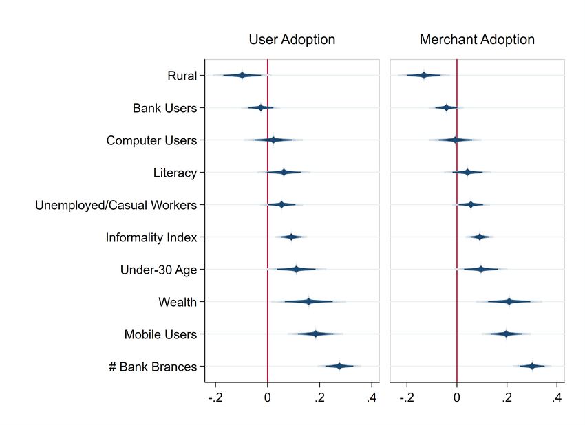
© 2020 International Monetary Fund                                                                   WP/20/138

                                          IMF Working Paper

                               Strategy, Policy and Review Department

    The Real Effects of Mobile Money: Evidence from a Large-Scale Fintech Expansion 1

                           Prepared by Manasa Patnam and Weijia Yao

                             Authorized for distribution by Vikram Haksar

                                                  July 2020

    Disclaimer: This document was prepared before COVID-19 became a global pandemic and
    resulted in unprecedented economic strains. It, therefore, does not reflect the implications of these
    developments and related policy priorities. We direct you to the IMF Covid-19 page that includes
    staff recommendations with regard to the COVID-19 global outbreak.

    IMF Working Papers describe research in progress by the author(s) and are published to
    elicit comments and to encourage debate. The views expressed in IMF Working Papers are
    those of the author(s) and do not necessarily represent the views of the IMF, its Executive Board,
    or IMF management.

                                                  Abstract

Mobile money services have rapidly expanded across emerging and developing economies and
enabled new ways through which households and firms can conduct payments, save and send
remittances. We explore how mobile money use can impact economic outcomes in India using
granular data on transactions from Paytm, one of the largest mobile money service provider in India
with over 400 million users. We exploit the period around the demonetization policy, which
prompted a surge in mobile money adoption, and analyze how mobile money affects traditional risk-
sharing arrangements. Our main finding is that mobile money use increases the resilience to shocks
by dampening the impact of rainfall shocks on nightlights-based economic activity and household
consumption. We complement these findings by conducting a firm survey around a phased targeting
intervention which incentivized firms to adopt the mobile payment technology. Our results suggest
that firms adopting mobile payments improved their sales after six-months of use, compared to other
firms. We also elicit firms’ subjective expectations on future sales and find mobile payment adoption
to be associated with lower subjective uncertainty and greater sales optimism.

JEL Classification Numbers: G20, G21, L25, L96, L86, O16, O33.

Author’s E-Mail Addresses: mpatnam@imf.org; wyao@imf.org

1
 The authors would like to thank Vikram Haksar, Tamim Bayoumi, Fabian Valencia, Gita Gopinath, Dong He,
Ranil Salgado, Alfonso Garcia Mora, Harish Natarajan, Andrea Presbitero, Purva Khera, Tomas Dutra Schmidt
and seminar participants at the IMF and World Bank. We also thank Katsiaryna Svirydzenka for many helpful
discussions during the early stages of this work. This work relied on the excellent co-operation with Paytm who
collected and provided the data for analysis. All errors and omissions are our own.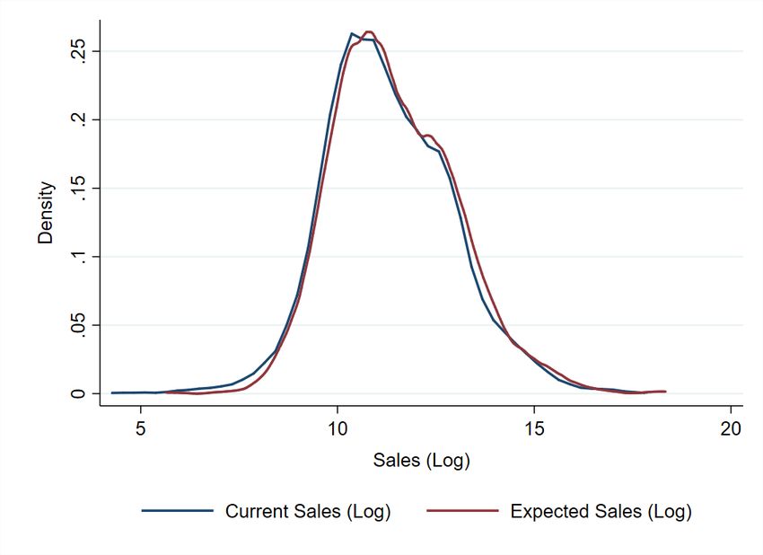
2

                                             Contents                                                                               Page

I.    Introduction . . . . . . . . . . . . . . . . . . . . . . . . . . . . . . . . . . . . . .                                           3
II.   Data on Transactions and Firm Survey . . . . . . . . . . . . . . . . . . . . . . . . 8
      A. Transaction level data . . . . . . . . . . . . . . . . . . . . . . . . . . . . . . 8
      B. Firm Survey around Intervention for Technology Adoption . . . . . . . . . . . 10
III. Empirical Strategy . . . . . . . . . . . . . . . . . . . . . . . . . . . . . . . . . . . 12
     A. Risk-Sharing Specification . . . . . . . . . . . . . . . . . . . . . . . . . . . . 12
     B. Effects of Mobile Payments Technology on Firms . . . . . . . . . . . . . . . 15
IV.   Results . . . . . . . . . . . . . . . . . . . . . .   .   .   .   .   .   .   .   .   .   .   .   .   .   .   .   .   .   .   .   16
      A. Who Uses Mobile Money? . . . . . . . . .           .   .   .   .   .   .   .   .   .   .   .   .   .   .   .   .   .   .   .   16
      B. Effects of Mobile Money on Risk-Sharing            .   .   .   .   .   .   .   .   .   .   .   .   .   .   .   .   .   .   .   18
      C. Effects of Mobile Money on Firm Sales . .          .   .   .   .   .   .   .   .   .   .   .   .   .   .   .   .   .   .   .   24
V.    Conclusion . . . . . . . . . . . . . . . . . . . . . . . . . . . . . . . . . . . . . . 30
References . . . . . . . . . . . . . . . . . . . . . . . . . . . . . . . . . . . . . . . . . . 32
3
I. I NTRODUCTION
Despite increased access to finance, the effective use of financial services remains low in In-
dia1 . The World Bank Global Findex Database (2017) 2 reports that only 20 percent of adults
in India save with a financial institution. Even within the population possessing a bank ac-
count, nearly half (48.5 percent) of the accounts remain inactive3 , making India the country
with the highest inactivity rate in the world in the 2017 survey. Moreover, only about 39 per-
cent of the survey respondents reported sending or receiving domestic remittances using a
financial institution. The bulk of remittance transfer are conducted with cash, either person-
ally or using the network of relatives and friends (Demirguc-Kunt and others, 2018).
Mobile money and digital wallets offer an innovative technological solution to fill the finan-
cial infrastructure gap and alleviate frictions related to the limited use of formal financial
services. This is because, the use of mobile money allows consumers to perform financial
transactions in a relatively inexpensive and reliable way (Jack and Suri, 2014), eliminating
spatial and temporal barriers, and can be used as a storage mechanism by both the banked and
unbanked (Morawczynski and Pickens, 2009). In India, Paytm has been the largest mobile
money payments firm since 2010, serving over 400 million users and 14 million businesses as
of 2019 (BusinessWorld, 2019).
In this paper, we examine the economic impact from the two distinct use cases of mobile
money, using large-scale data on monthly mobile money transactions of a little under half a
billion users in India. First, does it improve the resilience to economic shocks by enabling a
cheaper and more efficient way to save and transfer money? Second, can the adoption of this
relatively costless payment technology help increase the sales of micro and small enterprises
by reducing the frictions and costs associated with other payment methods. To investigate
these questions, we use data from one of the largest mobile money provider in India, Paytm,
and exploit (i) a policy episode which, by reducing the use of cash, suddenly increased the
nation-wide adoption of mobile money and (ii) the sequencing of a phased targeted interven-
tion that provided firms with an incentives to adopt the technology. In examining these ques-
tions, we aim to provide evidence on whether fintech innovations can have economy-wide
economic impacts, and do so in a setting with a large informal sector presence and where
considerable frictions to banking still exists.
Our investigation of the impact of fintech on economic outcomes is motivated, in part, by the
observation that the adoption of Paytm mobile wallets surged in the immediate aftermath of
1 Burgess and Pande (2005) document that between 1969 and 1990, bank branches were opened in roughly
30,000 rural unbanked locations. More recent evidence by Agarwal and others (2017) also show a large increase
in the number of households having access to the formal banking services,as a result of the government’s fi-
nancial inclusion program in 2014. However they find that 81 percent of the new consumers do not deposit any
money and 87 percent do not withdrawing any cash after opening the account. Finally, the World Bank Global
Findex Database reports that, in 2017, over 80 percent of adults in India possess a bank account.
2 Compiled using nationally representative surveys of more than 150,000 adults age 15 and above in over 140
economies. 3000 people were surveyed in India.
3 Inactive accounts are defined as not making any deposit or withdrawal within a year.4
the demonetization policy episode. This policy was enacted in November 2016, where the
Government of India unexpectedly announced the withdrawal of major banknotes from cir-
culation, effectively constraining the use of cash. Figure 1 plots the daily evolution of Paytm
transaction volumes six-months before and after the announcement of the policy. As shown in
the figure, there is a large spike in the level of transaction volumes immediately following the
policy announcement, which contrasts with the relatively lower level of transaction activity in
the days right before 4 . In contrast, the growth of debit cards transactions around this period
(October-December 2016) was 129 percent (RBI (2017 Feb)). Chodorow-Reich and others
(2020) also document a large increase in mobile money use following the demonetization
policy announcement. Crouzet, Gupta, and Mezzanotti (2019) further show that this increase
was persistent, in terms of the increase in the growth rate of the user base.
Figure 1. Paytm Use around the Demonetization Policy Period
The figure shows daily transaction volume from Paytm in blue (as an index with 1st May 2016 as base). The vertical dotted line
corresponds to the date of demonetization. We also show in red the counterfactual prediction calculated based on a Bayesian
structural time-series model (Brodersen and others, 2015), using proxies for economic/financial market activity growth in the post-
demonetization period (based on daily industrial production index, stock market index, and consumption index).
This large scale-up of mobile money in a relatively short period of time provides a novel ex-
perimental setting that allows us to compare periods with and without mobile money that are
4 Despite the distinct surge witnessed during demonetization, transaction volumes had been growing steadily
before; the average growth rate of monthly transaction volume of Paytm was 52 percent in the six months prior
to demonetization. It should also be noted that the level of transactions, attained from the adoption surge during
the demonetization episode, was broadly sustained through the subsequent years (2017 and 2018).5 in close proximity. With this in hand, we ask whether the negative effect of economic shocks, specifically rainfall shocks, can be mitigated by the use of mobile money, essentially testing for the regional risk-sharing benefits of mobile money. While the demonetization policy pro- vided an economy-wide impact, suddenly increasing mobile money adoption, our specific research question makes additional use of the exogenous timing of region-specific rainfall shocks. As can be seen in the figure above, the period before the policy announcement was characterized with very low levels of adoption and use that allows us to construct a ‘placebo’ period and test the counterfactual of whether high-adoption districts were also special in their risk-bearing capacities when hit by rainfall shocks. How can the mobile money innovation help improve risk-sharing outcomes? The principal implication of risk-sharing is that under complete markets, economic outcomes at the indi- vidual or regional level should respond only to aggregate economy-wide shocks and not to regional idiosyncratic shocks (Cochrane, 1991; Mace, 1991; Townsend, 1994). However the assumption of complete markets typically breaks down in a developing economy context where there are considerable frictions and market incompleteness in enabling risk-sharing arrangements. For instance, Kinnan and Townsend (2012) show that financial institutions help to some extent in smoothing consumption, but kinship networks play an important role too by providing indirect connections to the financial system when access is low. Jack and Suri (2014) show that mobile money innovation can help provide cheaper and more efficient alter- natives to risk-sharing by reducing the transaction costs associated with transferring resources. They find that mobile money has had a significant impact on the ability of households to share risk providing welfare benefits of on average 3 to 4 percent of income. Aron (2018) provides a review of the empirical evidence on mobile money and finds support for its role in improving risk-sharing. In addition to evidence from Jack and Suri (2014), no- table other studies such as Mbiti and Weil (2015) and Wieser and others (2019) find that the increased use of mobile money lowers the use of informal savings mechanisms and increases remittance transactions (respectively). Almost all of the existing empirical studies surveyed by Aron (2018), examine household-level outcomes with the impact of mobile money based typically on adoption (i.e., households with and without a mobile money account). However one limitation of micro-studies, as pointed out by Aron (2018), is that they may be a poor guide to the economy-wide effect of a policy in the presence of spillover effects and network- wide externalities. In addition to this concern, Aron (2018) also suggests the data used by the existing evidence, typically on number of users, is subject to measurement error as it may not reliably measure activity. The contribution of our paper is to examine the impact of mobile money on economy-wide outcomes by leveraging unique large scale data on mobile money transactions; to the best of our knowledge we are amongst the first to do so. Our analysis also addresses the data measurement issue by using data on both the number of users and transactions such that both, access to mobile money and its use, are measured precisely5 . More importantly, our data on 5 We also benefit from the fact that Paytm leads the digital payment landscape in India (GSMA, 2018), having singularly dominated the market during the demonetization period, such that our data accurately represents the overall mobile money adoption and usage.
6

district-wise peer-to-peer transactions, are split, both within and across districts allowing
us to explicitly test for the remittance channel through which mobile money can provide an
insurance against shocks. We find that while rainfall shocks have a significant negative impact
on economic activity, proxied by nighttime lights, – reducing it by 23 percent on average –
this effect is partially mitigated in districts that use mobile money. Specifically a 10 percent
increase in mobile money use in districts hit by a rainfall shock reduces the the negative effect
of the shock by 3 percent.

Our analysis of district-level risk-sharing also contributes to the broader literature on regional
risk sharing arrangements, as pioneered by Obstfeld (1995). The important role of finance in
enabling regional risk sharing arrangements is documented by Demyanyk, Ostergaard, and
Sørensen (2007) who find that the deregulation of U.S. banking restrictions, which increased
financial integration, improved interstate insurance. Hoffmann and Shcherbakova-Stewen
(2011) showing similar results also highlight the role of these deregulations in easing small
firms’ access to credit, essentially reducing financial access frictions and transaction costs.
We show in our paper that an innovative form of financial technology, mobile money, may
also serve the same purpose by reducing the cost of sending inter-region remittances, and in
this way improving financial integration to provide for better risk-sharing.

Our second question relates to more granular impacts at the firm level of enabling payments.
The ability to conduct payments through mobile phones is arguably an important and appeal-
ing feature that has contributed to the large scale take-up of mobile payment technology by
consumers and firms in several emerging and developing economies. For instance, in China,
mobile payments for consumption reached RMB 14.5 trillion (or 16 percent of GDP) in 2017;
Alipay (launched in 2004) and WeChat Pay (launched in 2011) now have over 500 million
and 900 million monthly active users, respectively, or 36 percent and 65 percent of the Chi-
nese population (Frost and others, 2019). In this context, we ask whether the adoption of
the mobile money payment technology6 can help increase the sales of micro and small en-
terprises by reducing the frictions and costs associated with other payment methods. The
theoretical literature on the adoption of electronic payments has highlighted a few channels
through which these effects may manifest. First, firms are likely to accept electronic modes
of payment, despite, in some cases incurring costly surcharge fees to avoid ‘missed sales’.
Bourguignon, Gomes, and Tirole (2019) describe missed sales as an occurrence when the
customer has a high inconvenience cost of paying by cash, and is discouraged by either a high
electronic payment surcharge or its non-acceptance. Bolt, Jonker, and Van Renselaar (2010)
report, from survey data in the Netherlands, that 5 percent of consumers leave a store without
purchasing when faced with card refusal or steep card surcharges. It is also possible that, in
the presence of full information, consumers never even visit stores that do not accept elec-
tronic payments (Chakravorti and To, 2007). Aggarwal, Brailovskaya, and Robinson (2019)
also posit that the improved transaction efficiency from the QR-code based payment technol-

6 The payment technology is based on the Quick Response (QR) code payment function in the mobile wallet,
which enables users to receive and make immediate payments by generating their own QR code on the mobile
phone app and complete a transaction by displaying or scanning QR codes. See Aggarwal, Brailovskaya, and
Robinson (2019) for more details on how this technology can improve payments efficiency.
7

ogy could promote demand, leading to a genuine increase in consumer spending and provide
evidence in favor of this.

Overall, this suggests that firms which are able to offer non-cash payment methods are likely
to either acquire new customers, increase the retention of old customers or spur customer de-
mand, thereby impacting sales. In the developing country context, there is an added effect of
transaction efficiency that may also lead to an increase in firm sales. Beck and others (2018)
study the effects of a payment technology innovation on entrepreneurship in a quantitative dy-
namic general equilibrium model, calibrating it with firm-level survey data from Kenya. They
show that the adoption of mobile money improves firm performance by allowing for more
efficient transfers, through the reduction in risky cash-holdings, and increased access to credit.
In their model, the improvements in firm performance deriving from payment technology
adoption lead to quantitatively significant macroeconomic effects.

To investigate this question, we take advantage of a phased targeting intervention that the
mobile money company, Paytm, conducts to incentivize firms to adopt their mobile app.
We exploit the sequencing of this intervention and identify ‘treatment’ and ‘control’ group
firms, with the former set of firm having experienced this technology for six months. We then
test the impact of this technology on subsequent firm sales using a difference in difference
strategy. Our results show that Paytm using firms improve their sales, by approximately 26
percent relative to firms non-Paytm firms, after six months of use. We also elicit subjective
expectations in our firm survey and and find that Paytm using firms have lower subjective un-
certainty around future sales. This complements our risk-sharing results at the district level on
consumption, suggesting that mobile money use can have sizeable volatility reducing effects
both at the firm and household level. These results are robust to different other methods of
identification such as matching on a large vector of location and other characteristics.

Our analysis of whether payment technology adoption benefits micro and small enterprises,
contributes to the broad literature on payment systems and, specifically, the still nascent
literature on financial technology adoption by firms in developing countries. There are few
empirical studies that directly study the effect of mobile payment technology on firm sales
and their subjective expectations. Dalton and others (2019) use a randomized control trial,
also incentivizing firms to adopt the technology, and find that adopting firms have better
access to finance and experience a reduction in sales volatility. Aggarwal, Brailovskaya, and
Robinson (2019) observe an increase in spending after the introduction of a mobile-payment
technology on other electronic payment methods such as, debit and credit card sales, which
promoted sales growth primarily for new businesses by facilitating customer acquisition.7
Our paper contributes to this nascent strand of literature and links directly the effect of mobile
payment adoption to the total sales of the firm (actual and future expectation) after six months
of use.

We now proceed to describing the data used in our analysis. The paper is organized as fol-
lows: in Section II we discuss the data obtained from Paytm records on users and transactions

7 Other
      studies include Aggarwal, Brailovskaya, and Robinson (2019) who find that mobile money adoption
among micro-enterprises raises their saving behavior and the likelihood of extending credit to consumers.
8
as well as the survey and intervention design for firm outcomes’ section III discusses the em-
pirical framework for testing the risk-sharing and payments technology effects on economic
activity and firm outcomes respectively; section IV reports the results obtained; Section V
concludes.
II. DATA ON T RANSACTIONS AND F IRM S URVEY
A. Transaction level data
We obtain data from Paytm on their monthly users and transactions at the district level.8 .
Our data is collected in total for 643 districts at a monthly frequency, between the time pe-
riod of May 2016- April 2019. The transactions relate to both offline payments9 and peer
to peer transfer10 and are disaggregated by value and volume. The payments data are fur-
ther disaggregated by payments made to formal and informal sector firms. The peer to peer
transfers data are further disaggregated by transfers made within a district and across-district
transfers11 . This enables us to identify remittance transfer from other districts in response to
idiosyncratic district specific shocks.
We merge the transactions data with two other principal sources of data. The first is data
on satellite measured night-time lights which we use as a proxy of district level monthly
economic activity (Henderson, Storeygard, and Weil (2011); Chen and Nordhaus (2011);
Kulkarni and others (2011); Alesina, Michalopoulos, and Papaioannou (2016)).The night
time image data is obtained from the Earth Observations Group (EOG) at the National Cen-
ters for Environmental Information. The EOG produces a suite of average radiance composite
images using nighttime data from the Visible Infrared Imaging Radiometer Suite (VIIRS)
Day/Night Band (DNB)12 . Prior to averaging, the DNB data is filtered to exclude data im-
pacted by stray light, lightning, lunar illumination, and cloud-cover13 . Each grid (one sq. km)
is assigned a pixel value which has a radiance unit14 . Luminosity is thus obtained as a sum of
lights over the gridded area which in our case is defined as the district, using GIS data on the
8 We use a list of total 654 districts, which is largely consistent with the 2011 Census of India.
9 All Paytm data relate to offline transactions i.e., excluding online transactions through websites or online retail
platforms. All other transactions conducted over the mobile phone and in physical shops are included under
offline transactions.
10 The peer to peer transactions data does not include a subset of these transactions made through the unified
payments interface which Paytm joined, beginning November 2017. To ensure comparability over different
time periods, we run the P2P analysis on data before November 2017, where these transactions were uniquely
identified.
11 Across district transfers for a specific district are defined as transfers received by this district from all other
districts in India.
12 The satellites collect a complete set of earth images twice a day. The data, in 15 arc-second resolution (1km
grid interval), covers the world from 75◦ North to 65◦ South latitude.
13 Cloud-cover is determined using the VIIRS Cloud Mask product (VCM). In addition, data near the edges of
the swath are not included in the composites (aggregation zones 29-32).
14 The radiance unit is the measured in W/cm2 and can be viewed as the intensity of electromagnetic radiation.9 administrative boundaries of states and districts. We then detrend this district-wise luminosity time-series to account for monthly seasonality. There are several reasons why we rely on luminosity data. The first is that monthly panel data on district GDP that could capture the evolution of incomes or consumption does not exist. The second reason is that, despite the measurement difficulties inherent in the use of such a proxy, there is convincing evidence to suggest that luminosity is strongly correlated with standard economic outcomes. Chaturvedi, Ghosh, and Bhandari (2011) and Bhandari and Roychowdhury (2011) examine this correlation at the district level in India and find similar effects. More recently Beyer and others (2018) measure monthly economic activity in South Asia at the district level using VIIRS lights data and find that for Indian districts, the luminosity measure has a high correlation with measured activity in national accounts. Finally, an additional reason for relying on luminosity evidence is that our identification strategy focuses on changes in outcomes rather than levels. This means that the sources of persistent heterogeneity across districts in the relationship between luminosity levels and levels of economic activity are not a concern. To corroborate our measure of night-time lights, we use additional data from the 2017-18 Periodic Labor Force Survey (PLFS) that provides various labor market measures in both the urban and rural areas across India. With the rotational panel sampling design of the survey, we were able to calculate average labor supply hours and per-capita expenditure on NSS region level15 for 4 quarters (July 2017 - June 2018)16 . The other key data we use are meteorological data on rainfall shocks, which serves as a mea- sure of a district-specific economic shock. The Indian Meteorological Department (IMD) collects rainfall data from about 3500 stations spread over the entire country, which provides the basis for compiling district-level rainfall statistics. The IMD also provides long-term rainfall averages for each district, based on the rainfall records for the period from 1951- 2000. We take the amount of deviation of each district’s current recorded level of rainfall in any given month from its long term average in the same month (positive or negative). We construct a binary indicator of rainfall shock taking the value one if the district’s rainfall is deficient or in excess of its long term average by 1.5 standard deviations of the cross-sectional distribution (roughly 100mm of rainfall). Essentially, it reflects conditions of either drought 15 Regions are hierarchical domains of study below the level of State/ Union Territory used in the surveys by National Sample Survey Organization. The average number of districts within a given NSS region is 7.3. 16 PLFS adopted a stratified multi-stage survey sampling design. First stage strata were formed within each NSS region. In urban areas, the strata are based on the size of towns and the rural strata are divided into sub-strata with similar population size. Then the first stage units (the Urban Frame Survey blocks in urban areas and the 2011 Population Census villages in rural areas) were selected within each strata/sub-strata by a Probability Pro- portional to Size with Replacement (PPSWR) Scheme. Finally, the second stage strata (within each first stage unit) were formed based on the number of members in the households with secondary or above education and certain number of households were selected from each second stage strata. To implement the 2-year rotational scheme, 8 samples of first stage units were drawn within each urban and rural strata/sub-strata. For each quarter, they canvassed (as first visits) 25 percent annual allocation of first stage units. The rural samples were only vis- ited once and the urban samples were re-visited 3 times in the subsequent quarters. But since the samples were drawn randomly, the data of each quarter should be representative at the NSS region level on average.
10

or flood within a district17 . Our analysis also conditions on district-wise bank availability. We
use quarterly data on the number of reporting / functioning offices at district level from the
Reserve Bank of India (RBI).

To explore descriptively the cross-sectional determinants of mobile-money use, and as Paytm
data are anonymized and stripped of any user or firm attributes, we gather data on district
level from various sources. Specifically, we use data from 2011 Census of India to calcu-
late some district-wise population characteristic measures such as share of rural households,
literacy rate and share of unemployed/casual workers. We also collect data on additional mea-
sures such as the share of households with bank accounts and the average wealth index from
the 2015 Demographic Health Survey by USAID. In addition, we construct an index of firm
informality at the district level based on data from the 2013 Economic Census of Establish-
ments18 .

                B. Firm Survey around Intervention for Technology Adoption

In addition to the data on transaction, we also collaborated with Paytm to conduct a survey to
obtain information on firm sales. The survey was designed around an intervention that Paytm
conducted to incentivize unregistered informal sector firms to adopt the payments mobile app,
enabling them to accept payments using a simple QR code19 . The incentives provided varied
but included cashback offers based on the first hundred payments received through the app
or Paytm Gold benefits. We provide further details of the intervention in section III.B and
discuss here the sampling and information collected through the survey.

The survey collected information on 3,046 firms out of which 1,417 belonged to the set of
firms that were targeted early in January 2019 (treatment group) and 1,629 belonged to the set
of firms that were targeted in July 2019 (control group). 925 out of the 3,046 firms provided
their sales figures for both the month before the survey and six months ago, which are crucial
to our analysis. The firms chosen to be surveyed were randomly sampled within each state by
treatment group.

The survey was designed to capture information on total firm sales for two sets of firms –
those that used the mobile payments technology and those that did not – six months before

17 We  check robustness to using continuous rainfall shock measures i.e., a district’s month-wise deviations from
its long-term average as in Bhalotra (2010). The pattern of our results is robust to using this measure but the
interpretation of risk-sharing parameters is less easy, compared to the binary measure.
18 Some variables in the Economic Census can help indicate whether this establishment is more likely to be for-

mal or informal business. We assigned points to these measures. And the informality level of each establishment
is measured by the sum of these points. Specifically, the points are: 1) type of house (1 point for "residential" or
"residential cum commercial"); 2) type of business ownership (1 point for "proprietary", "self help group" or "co-
operative"); 3) source of finance (1 point for "borrowing from non-institutions" or "loan from self help group",
2 points for "self finance"); 4) sector (1 point for "rural"); 5) number of workers (points = 1/"total workers"); 6)
share of non-hired workers (points = "non-hired workers"/"total workers").
19 Apart from the specific intervention for our analysis, firms can also adopt Paytm through their network of

colleagues/friends and perceived benefits to their business.
11
and after the former were incentivized to adopt. As the survey was conducted only once, we
asked firms to provide both their current monthly sales information as well as the amount of
sales from six-months ago on a recall basis20 . In addition to information on sales, we also
obtained data on other basic firm characteristics such as number of employees, business
category, whether they have access to a bank account and the amount of loan taken.
The survey also elicited information on firms’ subjective expectations on their future sales.
We asked each firm to report the minimum and the maximum monthly sales that they expect
to earn over the next year and the probability of earning more than the midpoint of the sup-
port of the distribution (Altig and others, 2019; Manski, 2004). The survey question was as
follows:
In the future, one year from now, what are your expectations about your business:
• What is the monthly maximum amount of sales that you think your business will be able
to earn, What is the monthly minimum amount of sales that you think your business will
be able to earn,
• On a scale of 0-10, with 0 being not at all likely and 10 being certainly likely, what is
the probability that your monthly sales in one year will be at least x [read out midpoint
the value from excel sheet]?
We then fit a triangular distribution to derive the mean (subjective expectation) and the stan-
dard deviation (subjective uncertainty) of future sales. The triangular distribution is typically
a more plausible description of the probability distribution of sales, because outcomes further
away from the midpoint receive less weight (see Guiso, Jappelli, and Pistaferri (2002) for a
discussion).
To cross-examine the reliability of the subjective expectations data, we compare the aver-
age future sales across the cross-sectional distribution of firms with the actual current sales
reported by them. Figure 2 plots the two distributions (in log values) which appear broadly
similar with the future sales distribution slightly shifted to the right suggesting some opti-
mism for the future.
20 The survey was conducted over two months which resulted in a small difference in the sales month for which
current and recall sales were asked between treatment and control group firms. For treatment (control) group, the
anchoring month for recall and current sales was February (January) and August (July) 2019. We use the World
bank BEEPS database for India, to investigate if there are seasonal differences in the sales growth based on the
one-month lag. We find a small positive sales differential such that the Jan-July sales differences is greater than
than the Feb-Aug sales difference. This suggests that if anything we should expect treatment group firms to have
a lower six-month sales growth differential.12
Figure 2. Distribution of Firm Sales: Current and Expected Sales
This figures plots the density of current and expected firm sales. The expected firm sales distribution is obtained from the cross-
section mean (first moment) of each firms’ subjective expectations distribution for future sales (one year ahead).
III. E MPIRICAL S TRATEGY
A. Risk-Sharing Specification
In this section we present our empirical test where we ask how the rainfall shock and cross-
sectional variation in mobile money use can affect economic activity, either as a way of sav-
ings for the unbanked or by allowing for faster and cheaper remittance transfer. We use the
following empirical specification to test for the risk-sharing effects of mobile money, using
night-time lights, Yit as a proxy of economic activity in district i at month t:
Yit = β Sit + γMit + δ Sit · Mit + χ Xit + αi + ηt + eit (1)
The variable Sit is a binary variable measuring the rainfall shock, as described in section II,
and reflects conditions of drought or flood within a district. We expect rainfall shocks (both
its surplus and deficit) to have a negative effect on economic activity.
The variable Mit measures the the intensity of Paytm use in district i in month t. We capture
intensity in two ways: first, we use the total number of users in a district at a given time;13 second, we make use of information on across and within district peer to peer transfers. Trans- actions linked to peer to peer transfers are directly related to the intensity with which indi- viduals transact among themselves, both within a given geographical area and across. The novel linking of transfers across districts allows us to examine the specific channel linked to across-district remittances in a district’s ability to smooth its weather shocks. However, since the rainfall shocks tend to be spatially heterogeneous even within a district, it is possible that, even the within district peer to peer transfer activity reflects to some extent the ability to share risk. Our hypothesis is that the negative effect of rainfall activity (i.e., β < 0) can be mitigated to some extent by efficient risk-sharing arrangements or some form of insurance. We test whether mobile money use can effectively serve this function by interacting the variable on rainfall shocks with mobile money use – the interaction term Sit · Mit in equation (1) – and examining the magnitude and significance of its coefficient δ . If indeed mobile money use can enable efficient risk-sharing arrangements then we would expect δ > 0 and the net shock- offsetting impact would depend on its magnitude. We supplement the empirical specification with a rich set of fixed effects, both cross-sectional and time specific. We employ district fixed effects (αi ) and either a full set of year by month effects or year and month effects separately (ηt ). This ensures that our results are robust to district-level time-invariant unobserved heteroegeneity as well as aggregate shocks over time. Since mobile money use tends to be highly correlated with banking activity, we also condition on the time-varying availability of bank branches in X (Burgess and Pande, 2005). Overall, our risk-sharing test predicates that β < 0 and δ > 0; further if informal risk-sharing arrangements are more effective than formal sector in finance then we would also expect δ > ζ . Identification of risk-sharing effects Our main identification restriction is for the rainfall shocks to be fully exogenous; specifically its timing and spatial occurrence to be orthogonal to mobile money use. There is one possibility that mobile money use is endogenously adopted in districts that are accustomed to rainfall shocks and already have good risk-sharing arrangements in place. In this case, our results would reflect the effect of these unobservable factors. To ensure our results are fully robust to this concern, we exploit the period around the demonetization shock use both an alternative identification strategy and a placebo test. The sudden and unexpected large-scale take-up of Paytm, in the immediate aftermath of the government announcement on demonetization gives us an ideal setting to identify a counterfactual period. We are able to compare, thus, a period in which most districts had very limited use of mobile money and a period succeeding it within days, where the same districts experienced a massive adoption surge. It is important to note that our analysis exploits only the nation-wide demonetization policy21 but still leaves room for district-specific rainfall shocks, which idiosyncratically impact economic activity. 21 Chodorow-Reich and others (2020) show a contraction in aggregate employment and night lights–based output due to the demonetization policy of at least 2 percentage points and of bank credit of 2 percentage points.
14

Leveraging the Regression Discontinuity Design: To address the concern around confounding
factors we make use of approaches based on the regression discontinuity design (RDD) which
exploits the arbitrarily narrow window around the demonetization policy. The assumption is
that within this interval, any unobserved factors related to a district’s risk-bearing capacity
are likely to be similar so that observations right before the demonetization episode, that led
to a spike in mobile money adoption, provide a comparison group for observations after. We
therefore augment equation (1) with a flexible district-specific polynomial time trend, P(t) · αi
(see Davis (2008) and Auffhammer and Kellogg (2011)) for a similar strategy):

                   Yit = β Sit + γMit + δ Sit · Mit + χXit + αi + ηt + λ P(t) · αi + eit                          (2)

We obtain consistent estimates of the risk sharing parameter, δ , from the RD specifications
above under the presence of time-varying unobservable factors related to a district’s risk-
bearing capacity, provided that the conditional mean of the unobservable is continuous around
the threshold. In other words, we expect that while unobservable factors jointly related to
the rainfall shock and mobile money use can affect economic activity, they do not change
discontinuously at the threshold of the demonetization policy episode.

In equation (2), the parameter ηt also includes a dummy variable indicating the period after
the demonetization policy was announce, to account directly for the impact of this policy
on economic activity. Note that as the policy announcement was both unexpected and im-
plemented at the aggregate level, the assignment variable – the district-specific time trend –
could not have been manipulated. In other words, unobservables related to economic activity
in districts could not have deliberately changed around the time cutoff in prior anticipation
of the policy. Our identification assumption is also more flexible than a standard RDD which
uses time as the assignment variable, but still exploits both cross-sectional and time varia-
tion through the timing of exogenous rainfall shocks.22 In this sense, our strategy is closer to
Lalive (2008) combining a difference-in-differences design with a regression discontinuity
design. In other words, we obtain the difference between a district’s economic activity when
hit by an exogenous district-specific rainfall shock by narrowly zooming in around the policy
announcement date, conditioning on the impact of the policy itself on economic activity.

Placebo test: Another way of ensuring robustness to confounding factors is to construct a
falsification exercise around the demonetization episode. To do so, we split the sample in two
periods - a period just before demonetization (pre) and a period right after (post). We then
artificially impute the post-demonetization district averages of mobile money use (M̄iPost in
the below specification) to the pre-sample.

22 Inline with the fuzzy RDD approach, we can also estimate equation (2) using an instrumental variable strat-
egy, by instrumenting the interaction term Sit · Mit with the interaction term which identifies rainfall shocks in the
post-demonetization period. In this set-up, we expect mobile money use to increase in districts hit with a rainfall
shock in the post-demonetization period (satisfying the instrument’s informativeness criteria) and for the latter
effect to be uncorrelated with unosbervables related to a district’s time-varying risk-bearing capacity in the close
time periods of pre and post demonetization (satisfying the instrument’s validity criteria). Our results are robust
to implementing this strategy.
15
YPre
it = β
Pre Pre
Sit + δ Pre SitPre · M̄iPost + χ Pre XPre Pre
it + αi + ηtPre + ePre
it (3)
If indeed, the districts that had intensive mobile money use were special in other dimensions,
then we would expect similar results in the pre-period, with δ Pre > 0, when mobile money use
was in fact quite limited.
B. Effects of Mobile Payments Technology on Firms
In this section we discuss our empirical strategy which examines whether the adoption of the
mobile QR code enable payment technology can improve firm sales. To do so, as described
in the introductory section we make use of the sequencing of a targeted intervention that
Paytm carried out to incentivize firms to adopt. We identify two sets of firms: firms who were
targeted for adoption in January 2019 (‘Treatment’ firms) and firms targeted six-months later
in July 2019 (‘Control’ firms). Both set of firms had not used the Paytm technology prior to
the intervention. The treatment group firms would have had approximately six-months of
experience accepting mobile payments, compared to the control group firms who, at the time
of the survey, had little to no experience.
Firms targeted for sign-up in:
January 2019 July 2019
(6 months with Paytm) (No Paytm)
Sales 6 months ago S0P (No Paytm) SC0 (No Paytm)
Sales current month S1P (Paytm) SC1 (No Paytm)
6 months Sales Growth ∆SP ∆SC
Treatment Effect ∆SP − ∆SC
This setup allows us to use a difference-in-difference identification strategy to test for the
six-month relative sales differential between treatment and control group firms:
Salesit = α · Treati + γ · Postt + β · Treati · Postt + eit (4)
where Salesit is the sales of the firm i at time t. The time t refers to either the pre-treatment pe-
riod where both sets of firms had no experience using the mobile payments technology, or the16
post-treatment period where the treatment group of firms had six-months of experience using
the technology. Correspondingly the variable Postt identifies the post-treatment period and the
variable Treati identifies the treatment group of firms. The relative sales growth differential is
given by the interaction term Treati · Postt .
As the intervention campaign only incentivized firms to adopt, with the decision to adopt
ultimately taken by the firms themselves, the effects identified by equation (4) represent intent
to treat effects (see for e.g., Crépon and others (2013)). The average treatment effects can be
recovered by using the intervention as an instrument for actual firm adoption; equation (4)
can then be estimated using two-stage least squares.
Identifying Assumption: The difference-in-difference specification relies on the common
trends assumption i.e., we should expect no sales growth differential between the two set
of firms, absent the intervention and adoption of the payments technology. To validate this
assumption we proceed in two steps. First, we recast equation (4) by adding fixed effects for
firms’ location (τi ) and business-type (bi ):
Salesit = α · Treati + γ · Postt + β · Treati · Postt + τi + bi + eit (5)
We then rely on a conditional common trends assumption and expect that both sets of firms
would have followed a common sales trajectory, conditional on being in the same location
and similar business groupings, in the absence of adopting the payment technology. In the
second step we use the subset of both treatment and control group firms that never-adopt the
technology despite being targeted in the intervention and check for their relative sales growth
differential. As these firms have absolutely no experience with mobile payments, we should
expect to see no difference in their sales between the pre and post period.
Finally, in addition to examining mobile money effects on firm sales, we also analyse whether
it can have an impact on how firm’s form expectation about future sales. For this we use the
measure of subjective probabilities elicited in the survey, as described in Section II. We then
fit a bi-triangular distribution on each firm’s subjective sales probability and derive the first
two moments of their future sales distribution. The first moment provides the firm’s forecast
of future sales, which we use with information on current sale to compute the impact of mo-
bile money on expected sales growth, using a similar specification as equation (5). We also
use the second moment to explore whether treatment group firms have lower subjective uncer-
tainty around future sales, after six-months of adopting the mobile payments technology.
IV. R ESULTS
A. Who Uses Mobile Money?
Before presenting the results on the impact of mobile money on aggregate economic activ-
ity and firm outcomes, we first explore the determinants of mobile money adoption across17 districts, leveraging the data on users and firms across the entire economy. We had shown pre- viously in Figure 1 that the demonetization policy episode, which constrained the use of cash provided a major economy-wide impetus for the take-up of mobile money. This could partly reflect the appeal of mobile money to ease transaction costs at a time when cash-constraints were severely binding. We now examine what factors - demographic, socio-economic and financial - drive the variation in mobile-money adoption across district, post the demonetiza- tion policy episode. Figure 3 plots the standardized correlation coefficients for consumer and firm adoption at the end of 2018. The figure shows that the determinants of both consumer and firm adoption are largely similar. The largest correlate of adoption is bank availability with a one standard devi- ation increase in the number of bank branches associated with a 0.2 to 0.3 standard deviation increase in consumer and firm adoption respectively. This high correlation, between the bank availability and mobile money use, could be explained by the banking-led model of mobile money in India In contrast to other countries (for e.g., Kenya) where mobile money users add money to their wallet though their telecommunication provider, in India mobile money wallets are largely linked to bank accounts23 . As expected, we also find that the number of mobile users within a district strongly predicts adoption24 . We find that mobile take up is relatively larger in districts with a younger population, with higher wealth and in urban areas. Yet, conditional on the factors described above, we also find that adoption is higher in areas with a larger proportion of unemployed and casual workers, suggesting an appeal amongst the unbanked population. Another similarly important finding, especially in the Indian con- text where the degree of informal sector activity is high, is the positive correlation of mobile money adoption and a district’s level of firm informality. As described in section II we con- struct the informality measure, directly based on the census of all firms domiciled within a district. We find evidence that a one standard deviation increase in a district’s informality increases the the take-up of mobile money by 0.1 standard deviation. 23 However, a person without a bank account can still add money to their mobile wallet through peer-to-peer transfers. It should be noted that since 2017, per the Reserve Bank of India guidelines, Paytm and other mobile operators are regulated as a Payments Bank. Such banks are primarily deposit-based and cannot issue loans and credit cards. 24 The strength of this variable’s correlation could be stronger than estimated, as we use data from the 2011 census to predict adoption rates in 2018. Given that the spread of mobile phones has increased significantly between the time periods, we expect there to be a larger correlation over time.
18

                              Figure 3. Determinants of Mobile Money Adoption

     This figures plots the standardized effects from a regression exploring the determinants of user and merchant/firm adoption. Data
     Source for the explanatory variables are: 1) Census 2011: Rural; Computer Users; Literacy; Unemployed/Casual Workers; Under-
     30 Age; Mobile Users; 2) DHS Household Survey: Bank Users; Wealth; 3) Economic Census 2013: Informality Index; 4) RBI: #
     Bank Branches

                                B. Effects of Mobile Money on Risk-Sharing

Table 1 presents results from our baseline risk-sharing specification, equation (1). The table
shows that a rainfall shock has a significant negative impact on economic activity – reduc-
ing it by 17 percent on average. However, this effect is partially mitigated in districts with
mobile money, depending on the intensity of use. Column (1) shows that the coefficient on
the interaction term of mobile money use and rainfall shock is positive and significant. A 10
percent increase in mobile money use in districts hit by a rainfall shock reduces the negative
effect of the shock by 3 percent. Column (2) conditions on the (log of) number of banks avail-
able in a district at time t, while Column (3) includes additionally fixed effects for each date
(month-by-year) in the sample period; the results are robust to the inclusion of different types
of controls.
19
Table 1. Effect of Mobile Money on Risk Sharing: Economic Activity
(1) (2) (3)
Rainfall Shock -0.169∗∗∗ -0.169∗∗∗ -0.184∗∗∗
(0.025) (0.026) (0.027)
Mobile Money 0.014∗∗∗ 0.017∗∗∗ -0.006
(0.002) (0.003) (0.008)
Mobile Money × Rainfall Shock 0.030∗∗∗ 0.030∗∗∗ 0.031∗∗∗
(0.004) (0.004) (0.004)
Bank Availability -0.363 -0.497
(0.282) (0.318)
Time Fixed Effects X
Observations 18827 18602 18602
r2 0.011 0.012 0.071
The table reports the average effects of rainfall shocks and mobile money adoption on economic activity. Mobile
money adoption is measured as the total log value of Paytm users in the district; the dependent variable for all
specifications is the demeaned log of the sum of night-time lights within each district. Standard errors clustered
at the district are reported in parentheses. * indicates significance at 10%; ** at 5%; *** at 1%.
Figure 4 shows how the risk-sharing effects vary by the intensity of mobile money use. For
instance, a district with lower tenth percentile value of transactions, can reduce the negative
effects of rainfall shock from 18 percent to 16 percent and this shock mitigating effect varies
depending on the level of use. A district with the median value of transactions, on the other
hand, can reduce the negative effects of rainfall shock from 18 percent to 1 percent.20
Figure 4. Risk Mitigation: Effect of Rainfall Shock by Intensity of Mobile Use
This figures plots the predicted marginal effects of rainfall shock at different cross-sectional percentile level of a district’s mobile
money adoption (10th, 25th and 50th percentile together with no mobile adoption). The effects with their 95 percent confidence
bands are reported in the graph.
As raised in the discussion in section III.A, there is still a possibility that mobile money is
endogenously adopted in districts that have good risk-sharing arrangements already in place
such that all the results in Table 1 simply reflect this. To ensure that our results are fully ro-
bust to this source of endogeneity, we conduct the additional falsification exercise exploiting
the period around demonetization. We split the sample into two – the period just before de-
monetization where Paytm was absent in most districts and the period after, when it expanded.
We then artificially impute the post-demonetization district averages of mobile usage to the
pre-sample and the idea is that, if indeed the districts that use mobile-money was special in
other dimensions, then we would expect the same results to hold-out in the period just before
demonetization, when in fact there was no mobile-money use. The results in Table 2, shows
that this is not the case, and in our placebo period we find the risk-sharing interactive term to
not just be insignificant but also reduced considerably in magnitude.21
Table 2. Effect of Mobile Money on Risk Sharing: Placebo Test & Robustnesss
Placebo RDD
Pre Post
(1) (2) (3) (4)
Rainfall Shock -0.209∗∗∗ -0.146∗∗∗ -0.204∗∗∗ -0.116∗∗
(0.078) (0.050) (0.025) (0.056)
Mobile Money × Rainfall Shock 0.008 0.025∗∗∗ 0.032∗∗∗ 0.026∗∗∗
(0.011) (0.006) (0.004) (0.005)
Time Fixed Effects X X X X
District-wise Time Trend Polynomial X X
Control for Post-Demonetization Period X X
Bank Availability & Shock Interaction X
Observations 3626 14976 7239 7239
r2 0.043 0.070 0.366 0.366
The table reports the average effects of rainfall shocks and mobile money adoption on economic activity. Mobile money adoption
is measured as the total log value of Paytm users in the district; the dependent variable for all specifications is the demeaned log
of the sum of night-time lights within each district. The pre period relates to the sample between May and October 2016, while
the post sample is for the six month period following the demonetization policy at the beginning of November 2016. RDD refers to
results from a specification with flexible district-wise polynomial time trends between the period May 2016 and April 2017. Standard
errors clustered at the district are reported in parentheses. * indicates significance at 10%; ** at 5%; *** at 1%.
As an additional robustness exercise, in column (3) of Table 2 we also use an alternative iden-
tification strategy exploiting the time period over the demonetization policy episode. The
regression discontinuity (RDD) specification used in column (3) fits a district specific poly-
nomial trend such that any unobservables (conditional on the aggregate post-demonetization
effect) related to risk-sharing are accounted for, to the extent that they do not change discon-
tinuously around the threshold. The sample used for estimating this specification also narrows
the time-window to six months before and after the policy episode. The results show that the
effect of mobile money in reducing the extent of rainfall shock still holds, both in magnitude
and direction. In column (4) we also include the interaction of bank availability with rainfall
shock, to mitigate the concern that mobile money adoption may be picking up risk-sharing
effects of banks, but the results remain robust to this inclusion.
Next, we relate our findings to the risk-sharing channel by using data on peer to peer transfers,
specially across-district transfers. In Table 3 we report additional results from the regression
discontinuity specification using peer-to-peer transfers to represent mobile money intensity.
The first column shows the same result (mobile money based on total users) from Column (3)
of Table 2. In column (2), using data on all peer-to-peer transfers received by a district, we
find a negative effect of the rainfall shock, which is partially mitigated by districts that receive
higher peer to peer transfers through mobile money. In column (3), we isolate only those peer-
to-peer transfers received by a district from other districts, removing therefore within-districtYou can also read