Analysis of short-period waves in the solar chromosphere
←
→
Page content transcription
If your browser does not render page correctly, please read the page content below
Analysis of short-period waves in the
        solar chromosphere

                       Dissertation
             zur Erlangung des Doktorgrades
   der Mathematisch-Naturwissenschaftlichen Fakultäten
        der Georg-August-Universität zu Göttingen

                      vorgelegt von
                 Aleksandra And̄ić
                  aus Banjaluka, Bosnia

                     Göttingen 2005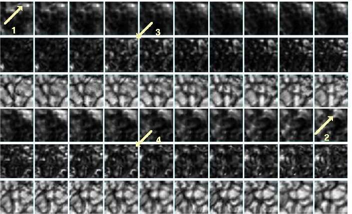
D7
Referent: Franz Kneer
Korreferent: Wolfgang Glatzel
Tag der mündlichen Prüfung: 06.07.2005
Contents

Summary                                                                                                                             5

1 Introduction                                                                                                                      7
  1.1 Heating of the solar atmosphere      .   .   .   .   .   .   .   .   .   .   .   .   .   .   .   .   .   .   .   .   .   .    8
  1.2 Acoustic waves . . . . . . . . .     .   .   .   .   .   .   .   .   .   .   .   .   .   .   .   .   .   .   .   .   .   .   10
       1.2.1 Propagation . . . . . . .     .   .   .   .   .   .   .   .   .   .   .   .   .   .   .   .   .   .   .   .   .   .   12
  1.3 Magnetic field effects . . . . . .   .   .   .   .   .   .   .   .   .   .   .   .   .   .   .   .   .   .   .   .   .   .   13
  1.4 Short-period waves . . . . . . .     .   .   .   .   .   .   .   .   .   .   .   .   .   .   .   .   .   .   .   .   .   .   14

2 Observations                                                                                                                     15
  2.1 Aim of the observations . . . . . .      .   .   .   .   .   .   .   .   .   .   .   .   .   .   .   .   .   .   .   .   .   15
      2.1.1 Choice of the spectral line        .   .   .   .   .   .   .   .   .   .   .   .   .   .   .   .   .   .   .   .   .   15
  2.2 Instrumentation . . . . . . . . . .      .   .   .   .   .   .   .   .   .   .   .   .   .   .   .   .   .   .   .   .   .   17
      2.2.1 Telescope . . . . . . . . .        .   .   .   .   .   .   .   .   .   .   .   .   .   .   .   .   .   .   .   .   .   17
      2.2.2 Post-focus setting . . . . .       .   .   .   .   .   .   .   .   .   .   .   .   .   .   .   .   .   .   .   .   .   18
  2.3 Data . . . . . . . . . . . . . . . .     .   .   .   .   .   .   .   .   .   .   .   .   .   .   .   .   .   .   .   .   .   20
      2.3.1 Observations . . . . . . .         .   .   .   .   .   .   .   .   .   .   .   .   .   .   .   .   .   .   .   .   .   22

3 Data reduction and analysis methods                                                                                              23
  3.1 Data reduction . . . . . . . . . . . . . . . . . . .                     .   .   .   .   .   .   .   .   .   .   .   .   .   23
       3.1.1 Speckle reconstruction . . . . . . . . . .                        .   .   .   .   .   .   .   .   .   .   .   .   .   24
       3.1.2 Reconstruction of the narrowband images                           .   .   .   .   .   .   .   .   .   .   .   .   .   26
  3.2 Determination of the heights . . . . . . . . . . .                       .   .   .   .   .   .   .   .   .   .   .   .   .   27
       3.2.1 Bisectors . . . . . . . . . . . . . . . . .                       .   .   .   .   .   .   .   .   .   .   .   .   .   27
       3.2.2 Response functions . . . . . . . . . . . .                        .   .   .   .   .   .   .   .   .   .   .   .   .   27
       3.2.3 Velocity maps . . . . . . . . . . . . . . .                       .   .   .   .   .   .   .   .   .   .   .   .   .   32
  3.3 The data cubes . . . . . . . . . . . . . . . . . .                       .   .   .   .   .   .   .   .   .   .   .   .   .   33
       3.3.1 Correlation . . . . . . . . . . . . . . . .                       .   .   .   .   .   .   .   .   .   .   .   .   .   33
       3.3.2 Destretching . . . . . . . . . . . . . . .                        .   .   .   .   .   .   .   .   .   .   .   .   .   34
  3.4 Wavelet analysis . . . . . . . . . . . . . . . . . .                     .   .   .   .   .   .   .   .   .   .   .   .   .   35
       3.4.1 The mother wavelet . . . . . . . . . . . .                        .   .   .   .   .   .   .   .   .   .   .   .   .   35
       3.4.2 The code . . . . . . . . . . . . . . . . .                        .   .   .   .   .   .   .   .   .   .   .   .   .   36
       3.4.3 Additional data processing . . . . . . . .                        .   .   .   .   .   .   .   .   .   .   .   .   .   37

                                                                                                                                    3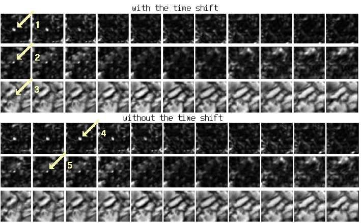
Contents

4 Results                                                                                                                                              39
  4.1 Waves at different heights . . . . . . . . . . . . . . . . . . . . . . . . . .                                                                   39
       4.1.1 Spatial location . . . . . . . . . . . . . . . . . . . . . . . . . . .                                                                    41
  4.2 Methods used for the analysis of the data . . . . . . . . . . . . . . . . . .                                                                    42
       4.2.1 Comparison of the spatial distribution of short-period waves with
              white-light structures . . . . . . . . . . . . . . . . . . . . . . . .                                                                   43
       4.2.2 Determining the time shift . . . . . . . . . . . . . . . . . . . . .                                                                      46
       4.2.3 Different periods . . . . . . . . . . . . . . . . . . . . . . . . . .                                                                     48
       4.2.4 Terms used for description of granular events . . . . . . . . . . .                                                                       49
  4.3 Location of short-period waves . . . . . . . . . . . . . . . . . . . . . . .                                                                     50
       4.3.1 The quiet Sun . . . . . . . . . . . . . . . . . . . . . . . . . . . .                                                                     50
       4.3.2 Solar area with G-band structures . . . . . . . . . . . . . . . . .                                                                       53
       4.3.3 Observations containing a pore . . . . . . . . . . . . . . . . . . .                                                                      54
  4.4 Relation of short-period waves to certain structures on the Sun . . . . . .                                                                      56
       4.4.1 The quiet Sun . . . . . . . . . . . . . . . . . . . . . . . . . . . .                                                                     56
       4.4.2 Solar area with G-band structures . . . . . . . . . . . . . . . . .                                                                       57
       4.4.3 Observations containing a pore . . . . . . . . . . . . . . . . . . .                                                                      58
  4.5 Relation between waves of different periods . . . . . . . . . . . . . . . .                                                                      59
       4.5.1 Variation of power location with periods . . . . . . . . . . . . . .                                                                      60
       4.5.2 Comparison of short-period waves with waves of the longer-period                                                                          63
  4.6 Travelling of waves through the solar atmosphere . . . . . . . . . . . . .                                                                       66
       4.6.1 Matching of similar power features . . . . . . . . . . . . . . . .                                                                        67
  4.7 Energy transport and the dissipation of energy . . . . . . . . . . . . . . .                                                                     74

5 Summary and conclusions                                                                                                                              79
  5.1 Location of power . . .              .   .   .   .   .   .   .   .   .   .   .   .   .   .   .   .   .   .   .   .   .   .   .   .   .   .   .   79
  5.2 Periods . . . . . . . .              .   .   .   .   .   .   .   .   .   .   .   .   .   .   .   .   .   .   .   .   .   .   .   .   .   .   .   80
  5.3 Travelling . . . . . . .             .   .   .   .   .   .   .   .   .   .   .   .   .   .   .   .   .   .   .   .   .   .   .   .   .   .   .   81
  5.4 Energy . . . . . . . . .             .   .   .   .   .   .   .   .   .   .   .   .   .   .   .   .   .   .   .   .   .   .   .   .   .   .   .   81

6 Suggestions for future investigations                                                                                                                83
  6.1 Instrumental . . . . . . . . . . . . . . . . . . . . . . . . . . . . . . . . .                                                                   83
  6.2 Information from the granular pattern . . . . . . . . . . . . . . . . . . .                                                                      83
  6.3 Information from the line profiles . . . . . . . . . . . . . . . . . . . . . .                                                                   83

A Appendix 1                                                                                                                                           87
  A.1 Fabry- Perot interferometer . . . . . . . . . . . . . . . . . . . . . . . . .                                                                    87

B Appendix 2                                                                                                                                           89
  B.1 2003 .     . . . . . .   .   .   .   .   .   .   .   .   .   .   .   .   .   .   .   .   .   .   .   .   .   .   .   .   .   .   .   .   .   .   89
  B.2 2004 .     . . . . . .   .   .   .   .   .   .   .   .   .   .   .   .   .   .   .   .   .   .   .   .   .   .   .   .   .   .   .   .   .   .   89
      B.2.1      22.6.2004     .   .   .   .   .   .   .   .   .   .   .   .   .   .   .   .   .   .   .   .   .   .   .   .   .   .   .   .   .   .   89
      B.2.2      26.6.2004     .   .   .   .   .   .   .   .   .   .   .   .   .   .   .   .   .   .   .   .   .   .   .   .   .   .   .   .   .   .   90

Acknowledgements                                                                                                                                       95

Curriculum Vitae                                                                                                                                       97

4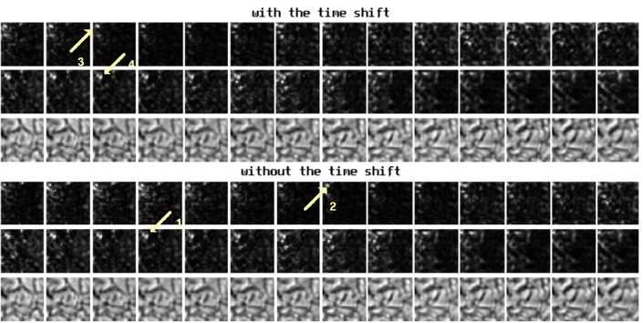
Summary

The temperature of the solar atmosphere decreases to low values of                  K at approxi-

mately  km height above   and then increases to approximately                    K around

        km height. This phenomenon can only be explained by mechanical heating of the
chromosphere. Short-period acoustic waves were suggested as the source of the mechan-

ical heating; waves with periods between  s and  s are assumed to be the main car-
riers of the required energy. Those waves originate in the sub-photosphere. Propagating
through the solar atmosphere, they form shocks and thus dissipate energy.
      Observations for this work were done with the telescope Vacuum tower Telescope
(VTT) at the Observatorio del Teide, Tenerife. The data reduction is done with speckle
interferometry. The velocity response functions are calculated using the LTE atmospheric
model (Holweger & Müller 1974) for an estimate of the heights. The results are obtained
with wavelet analysis.
      Short-period waves exist at different heights and are located mostly above down flows.
They closely follow the temporal evolution of the white-light structures. The short-period
waves of different periods seem to be associated with different spatial scales.
                                                                           "!
      The velocity interval of short-period wave propagation starts with                   # but the
upper limit can not be determined with the temporal resolution achieved in this work. The
magnetic field has an influence on the propagation of short-period waves.

      The energy flux at the height of           km is:
                                                              +,
                                     $ %'&'&         *
                                                )(        ( - %

The energy flux at the height of (         km is:
                                                             +,
                                     $ .'&'&        *
                                                           %
                                               /           -

And the difference between those two energy fluxes is:
                                                              +8,
                             $0%'&'&213$0.'&'&     567
                                               4           - %

This difference could represent the energy flux which is used for heating of chromosphere
or the energy flux which simply returned to the photosphere. The interpretation depends
on the adopted location of the chromospheric base.

                                                                                                  5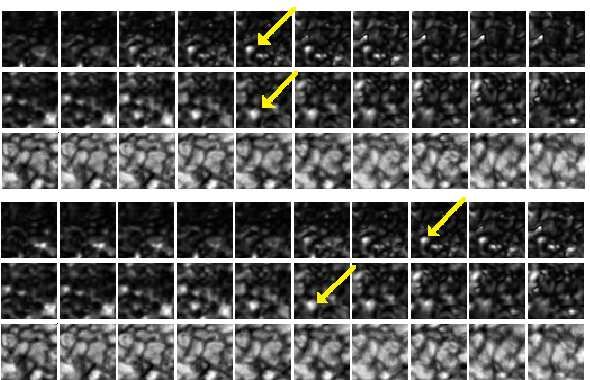
1 Introduction

The Sun is an average star of spectral type G2. The mean distance between the Sun and the
1 Introduction
1.1 Heating of the solar atmosphere
As mentioned above, we can observe in the chromosphere an increase of the temperature
with the height above the temperature minimum. The chromosphere radiates more light
G 1 LK
than it% absorbs from below. The radiative loss for the chromosphere is F (HAIJ
,3M -
, the uncertainty being caused by the differences of energy losses in quiet and
active regions 1 (Kneer & Uexküll% 1999). The heating required to balance the radiative
KN,3M - 2
loss is approximately I (Kalkofen 2001). According to (Kalkofen 2001) the
chromospheric temperature averaged over the time does not increase with height, and one
can say that the problem of chromosphere heating is a question of energy supply for the
radiative emission.
As source for the heating of the solar atmosphere one has to consider the convection
zone. All late type stars with surface convection zones are believed to have hot chromo-
spheric layers where the temperature increases outwards from low photospheric values to
OQP
about . It is believed that unresolved motions, or non-thermal micro-turbulence may
be responsible for the energy transport to the chromosphere.
An amount of heat RS entering into a volume element across its boundaries raises the
MV V
entropy T by RLT)URS , where is the temperature. For a gas element moving with
sound velocity W through the chromosphere, we have an entropy conservation equation
written in the Lagrange frame (Ulmschneider & Kalkofen 2003):
M M M M M M M M
RLT RX
)YZT Y8X[\WLYZT YJ]\:RLT RX_^a`b[cRLT RX_^edZ[cRLT RX_^af2[cRLT RX_^agh[\RGT R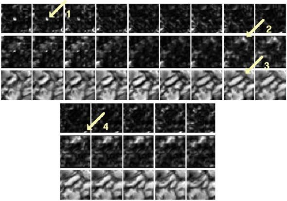
1.1 Heating of the solar atmosphere
quiet regions, they can thus be ignored. Since the chromosphere does exist, there should
be a mean steady state, and the left hand side of Eq. 1.1 should be zero. So we can write:
k l
1p RGT
m V Fon H[
R
1 Introduction

Figure 1.1: Behaviour of waves with height with thermal conduction neglected. Solid
lines represent flux, dotted lines dissipation, (Stein & Leibacher 1974).

1.2 Acoustic waves
Below the photosphere, a convective layer exists from which overshooting plasma is vis-
ible as the ’solar granulation’ (see Fig. 1.2). There are several possibilities how the con-
vection zone may generate the wave modes in the atmosphere: a) convective motions pen-
etrate into atmospheric layers and directly deposit their energy; b) pressure fluctuations,
generated by convective motions, propagate as acoustic waves; c) thermal over-stabilities,
which occur in the upper layers of the convection zone, generate waves.
    The second possibility is widely accepted as the method of generation of acoustic
waves. The generation of acoustic waves can be described by the ’Lighthill mechanism’
(Lighthill 1951). The most energetic oscillations should be generated in those regions
where the convective velocities are largest. The more detailed explanation one can find
also in (Proudman 1952) and (Stein 1967). Some authors argue that short-period bursts
are either generated by rising granules, or propagate more or less uniformly from deeper
layers into the convection zone (Deubner & Laufer 1983). Although there is a general
consensus that the source of acoustic waves is convective motion, some authors argue that
one can not decide whether their origin is convective or magnetic. The observational and
the theoretical results do not reveal a clear picture of the source of the solar oscillations
(Moretti et al. 2001).
    The frequencies of the acoustic waves depend on various parameters of the fluid flow:

10
1.2 Acoustic waves
Figure 1.2: One of the broadband images taken with the Vacuum Tower Telescope (VTT)
at the Observatorio del Teide (OT), Tenerife, after speckle reconstruction. One can see
the granulation pattern of surface convection. The field of view is 1 Introduction
of solar waves is associated with a rapid cooling occurring in the upper convection layer.
Indeed, events which last a few minutes and extend over an area of a few arcsec have
been detected to follow a darkening and a collapse of the plasma which is localized in
the intergranular lanes (Espagnet et al. 1996). The most energetic waves are associated
with those down-flows in dark areas which are well separated from each other in time and
space (Espagnet et al. 1996). Some observers noticed strong waves following expansions
of intergranular spaces. There is observational evidence that acoustic waves tend to be
converted into magneto-acoustic waves at locations where a magnetic field is expected,
e.g. at granular boundaries or in bright points (Espagnet et al. 1996). There are also
suggestions about a transition from acoustic waves in the centres of supergranulation cells
to fast magneto-acoustic waves at the boundaries of supergranulation or chromopshere
network. (Kalkofen 1990)
Kalkofen (1990) suggests that the location of acoustic waves should depend on their
frequency. In areas of strong magnetic fields at the cell boundary, Kalkofen calculates that
1
heating is done by waves of ( min periods. The bright points are heated by waves
-¿¾
with periods around ª ; locations free of magnetic field will be heated by waves of
still shorter period.
1.2.1 Propagation
In the solar atmosphere the acoustic transit time is approximately 5 minutes (for a height
of km and a sound speed of kms ÀÂÁH , which match with the period of the min
oscilations. For a propagation of acoustic waves in the solar atmosphere over several
scale heights, their frequency has to be above the cut-off frequency:
J®
¯ Ã « Ä j (1.8)
#
® Ä M Ä Ä
where
Å is the gravitational acceleration, y is the adiabatic coefficient and #
J® ³
C is the sound speed, with C as density scale height:
1 m &
CÇÆ £È j (1.9)
oÉ
(see: Stix (2002), chapter 5.2.4). The cut-off frequency varies with the height in the
® Ä
atmosphere since and # are not constant. Thus, at a certain height in the atmosphere a
® Ä
reflection layer exists where the values of and # yield the appropriate cut-off frequency.
For a given frequency, a wave can be propagating at one height and be evanescent at
other. This means that for waves of different frequency, the atmospheric conditions -
temperature and density stratification form reflection layers at different heights. Waves
can freely propagate below the reflection layer where their frequency reaches the local
cut-off frequency. At the corresponding reflection layer they are reflected downwards.
This situation can cause standing waves for almost the whole range of acoustic waves.
Fleck et al. (1989) explain that there is a possibility for standing waves, originating from
the total reflection of upward propagating waves at the chromosphere - corona transition
region. This discovery of standing patterns was confirmed by Espagnet et al. (1996).
Waves with a frequency above the atmospheric cut-off frequency ¯bà (Eq. 1.8) propa-
gate across the temperature minimum towards the chromosphere and corona. As long as
121.3 Magnetic field effects
$
Ê
the wave amplitude is small, the energy flux associated with propagating waves is
%
$0Ê Ä m
# W j (1.10)
Ä
where # is the speed of sound, m the mass density, and W the velocity fluctuation of%ÍÌ the gas.%
$0Ê ÄË º Ä m ÀÂÁuÎ
Since #
ª X and depends only weakly on the temperature we have W
meaning that the velocity fluctuations increase through the chromospheric layers. We can
Ä Ä
assume that # is constant above Mm. For small amplitudes, we have WÏB #.
During propagation through the solar atmosphere the velocity amplitude increases
with decreasing density. The wave crests start to travel with different velocities as com-
pared to wave valleys. This yields a deformation of the wave affecting a saw tooth shape
and the creation of a shock front where the energy is dissipated; an illustration of this
process can be seen in Fig. 1.4.
Figure 1.4: Sketch of acoustic-wave propagation through the solar atmosphere.
The propagation of waves through the atmosphere will cause a height-dependent vari-
ation of its frequency. These changes are caused by the resonance property, the merging of
shocks, and from shocks ’cannibalizing’ each other. As a consequence of this behaviour,
the spectrum develops at km height into almost pure 3 minute spectrum. Above
km, the chromosphere reaches a dynamical steady state where the mean tempera-
ture is time-independent (Ulmschneider 2003). The acoustic wave then travels on top of
this mean temperature, while its shock dissipation continuously provides the energy for
the chromospheric radiation losses.
1.3 Magnetic field effects
One usually defines as quiet Sun those areas where the solar magnetograms do not show
locations where polarisation signals exist. But recent research (Domı̀nguez 2004) has
131 Introduction
shown that the quiet Sun is not at all magnetically quiet. Indeed, besides the visible mag-
netic structures, there are also the magnetic knots. Their life time is approximately one
hour and they typically appear in dark intergranular lanes; and therefore can be associated
with the down-flow motions. Magnetic knots are flux concentrations and can be seen in
the spectrum as the line gaps.4 Therefore, in those areas one can expect strong mixture of
the acoustic waves and Alfvén waves.
pÑÐ O
It was general consensus that the magnetic field in the quiet Sun around À T
pÒÐ
and for active regions it is assumed that magnetic field has values from T till
pÓÐ 5
T in Sunspots (Stix 2002). In a recent analysis of the quiet Sun magnetic fields,
Domı̀nguez (2004) observes elements in the quiet Sun with magnetic field strengths of
pÐ K
the order of T, and that % of the areas having the magnetic field around À T.
In magnetic locations, the waves may travel with Alfvén speed. The velocity for
Alfvén waves can be calculated with the expression:
p %
WÕÔ> k m j (1.11)
p
where is the magnetic field and m the density of the atmosphere. It is clear that the
velocity of Alfvén waves will follow variations in the magnetic field.
The correlations of chromospheric losses with concentrations of the magnetic fields
suggest that the field should play a role in the heating. In a flux tube, the analogue to
the ordinary acoustic wave is the longitudinal tube wave. Longitudinal tube waves are
produced by fluctuating compressions of the magnetic tubes. They are very similar to
acoustic waves and develop into shocks, which heat the tubes by dissipating the wave
energy. The main influence of the magnetic field comes from its geometric shape which
channels the propagating wave. The narrower the channelling, the stronger the upwards
increase of the amplitude, and therefore the deeper the level where shock formation and
heating occurs.
1.4 Short-period waves
In the previous few years, short-period waves were detected. But it was not clear whether
they are propagating through the atmosphere and carry enough energy flux to cover the
needs of the chromosphere. Hence, an analysis of short-period waves was necessary.
Ulmschneider (1971b) predicted the maximum of the transported energy for the waves
2 Observations

2.1 Aim of the observations
Short-period waves are thought to carry the energy needed for the heating of the chromo-
sphere. Their detection and analysis is a vital step in solving this puzzle about heating.
    Short-period waves are spatially small events and their temporal changes are quite
rapid. In order to observe such short-period waves one needs high spatial and temporal
resolution. The high temporal resolution requires a fast repetition rate; a high spatial
resolution is achieved from best observations combined with special techniques for data
reduction.

2.1.1 Choice of the spectral line
Since acoustic waves are supposed to heat the chromosphere, the first request was to ob-
tain information which is not influenced by the magnetic field. To prevent strong thermal
broadening, spectral lines of elements with large atomic mass should be chosen. Tak-
2 Observations
2.2 Instrumentation

                                             ¥
length of the acoustic waves is smaller than ] the line shows no wavelength fluctuations
but only a line broadening. This fact limits observations to waves with periods greater
      ¹
2 Observations
the telescope is less extended than at sea level. At the Canaries, telescopes are additionally
located above the mean height of the cloud layers. Another factor is the wind which may
remove atmospheric turbulences. Long distance influences of the Earth’s atmosphere are
further improved by the location on an isolated island far from larger land masses. For
solar telescopes it is additionally useful to have surroundings which are not much heated
during the day. Heating of the immediate telescope surrounding is minimized by reflective
material and white colour of the building.
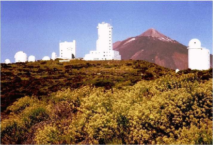
The VTT (see Fig. 2.3) was built on such an appropriate site. It is located at _( » á
= =
geographical longitude and » á latitude, thus often exposed to trade winds. Several
hundred meters below the telescope, a stable cloud layer usually forms a helpful temper-
ature inversion layer.
Figure 2.3: Open dome of VTT (Vacuum Tower Telescope)
=
The VTT is equipped with a coelostat system, having two mirrors of cm size. The
main imaging mirror has cm diameter and a focal length of ( m. The main optical path
is protected by a vacuum tube preventing air convection due to the vertical temperature
stratification in the most sensitive parallel beam.
2.2.2 Post-focus setting
As mentioned above, this work requires data which will contain spectral information.
Two-dimensional spatial maps at several spectral positions in the line profile appeared
to be optimal for the present work. Besides a fast repetition rate between scans through
the line are required. A post-focus instrument which meets all the requirements is the
Göttingen Fabry-Perot spectrometer (Bendlin et al. 1992). With this instrument, and an
appropriate set of reconstruction methods, the high temporal and spatial resolution neces-
sary for my work could be achieved.
182.2 Instrumentation
The Göttingen Fabry-Perot is located in the optic laboratory No. 2 of the VTT. The
light from the main path of the telescope is deflected into that ’OL2’ by means of a
mirror. The complete scheme of the post-focus setting is shown in Fig. 2.4.
Figure 2.4: Schematic view of post-focus settings used to obtain the data for this work.
The scheme of Fig.2.4 shows the instrumentation in two rooms, the main observing
room and the optic laboratory No.2, both are separated by the dashed line marked as ’the
wall’. Those parts of the instrumentation located in the main observing room, marked as
HBR, consist of a mirror M1 which deflects the light to a camera, an imaging lens and
two filters, the one marked IF3 being a ’G-band filter’ (i.e., set at the CH absorption near2 Observations
observations, mirror M2 is outside the beam. Mirrors MM3 and MM4 with adjoining
equipment are used for fine tuning of the FPIs.
=
Both cameras are slow scan ones and have Thompson TH 7863 FT chips with ¼
=
( pixels. FPI1 is a Queensgate etalon ’ET 100’ with an aperture of mm, â m spac-
¹
ing and a finesse of ã 40. FTP2 has an aperture of mm, its spacing can vary from
¹
â m to several mm. It has a finesse of ã 30 and is manufactured by Burleigh Instru-
ments Ltd (Koschinsky et al. 2001). Reflections between two FPIs can cause reflexes on
CCD2; to avoid this, FPI1 is slightly inclined against the optical axis. Some additional
information about the FPI can be found in Appendix A.
2.3 Data
In this work data sets from several observation campaigns were used. The direction of
the FPIs scanning was done for all lines from the red to the blue. The data set, DS1, was
taken by J.K. Hirzberger and M. Wunnenberg during August 2000 (Wunnenberg 2003).
The rest of the data sets were taken during observational campaigns in the years 2003 and
2004, see Table 2.3. The main objective was to achieve the fastest repetition rate possible,
allowing to study waves with shortest periods. Since the time evolution of short-period
waves was of main interest, reasonably long time sequences were taken.
Table 2.3: Dates, used lines and object of observation for obtained data sets.
Data Sets
mark date line used object of observation
DS2 08.10.2003 543.45 nm and 543.29 nm quiet Sun, disk centre
DS3 22.06.2004 543.45 nm and 543.29 nm quiet Sun, disk centre
DS4 24.06.2004 543.45 nm and 543.29 nm quiet Sun and G-band structures
disk centre
DS5 25.06.2004 543.45 nm and 543.29 nm pore, disk centre
DS6a 26.06.2004 543.45 nm quiet Sun, disk centre
DS6b 26.06.2004 543.45 nm pore, disk centre
DS7 28.06.2004 543.45 nm quiet Sun and G-band structures
disk centre
During the October 2003 campaign it was decided to observe with two lines. The
main reason was the expectation that noise will less influence the final results if two lines2.3 Data
In the campaign of June 2004, the adaptive optics (Berkefeld & Soltau 2001, Soltau et
al. 2002) could be used; these data sets were obtained with the help of J.K. Hirzberger, S.
Stangl and K.G. Puschmann. During this campaign some data sets were taken with one
and some with two lines (see Table 2.3). Additional details about each data set obtained
with two lines can be seen in Table 2.4. During this observation campaign various solar
regions were observed. To determine the correct area the equipment from HBR is used.
The areas which showed neither G-band structures nor other magnetic activity were cho-
sen as the Quiet Sun. For the active areas the field of view with the pores and with large
number of G-band bright points were chosen. The coordinates represent the position of
the field of view, in arcsec, where the reference point is the centre of the Sun. During the
take of data the FPIs move through the selected spectral line with previously determined
steps. The number of steps and the position in the line where the FPI will pause for taking
images is pre-determined. Those numbers of places in the line are in Table 2.4 and 2.5
marked as line positions. One complete FPI pass through the spectral line is called scan.
The FPIs have a limited range of scanning. In the case that more than one spectral line
will be scanned, it is sometimes necessary to skip the area between the lines. To achieve
that, the FPIs are set to perform a jump. At the given line position the FPIs jump over
the predetermined distance. The cadence indicates the repetition time of the FPI scans
through the total spectral range.
Table 2.4: Details for obtained data sets for two lines.
Data Sets
mark coordinates images line positions exposure time jump at cadence
[arcsec] per scan [ms] [s]
å
DS2 ä j 108 18 30 10 27.4
å
DS3 ä j 108 18 30 10 28.2
å
DS4 ä j 108 18 30 10 28.4
å
DS5 ä j 108 18 30 10 28.3
Since the repetition rate of data sets with two lines was rather low, I took additional
data sets with only one line to achieve a faster repetition rate, see Table 2.5.
Table 2.5: Details for obtained data sets for one line.
Data Sets
mark coordinates images line positions exposition cadence
[arcsec] per scan [ms] [s]
; ;GæÕå
DS6a ä ( j 91 13 20 22.7
;5= 1 å
DS6a äç j 91 13 20 22.7
å
DS7 äe(j 91 12 20 29.9
The last data set, DS7, was taken to check whether the number of images per scan has
212 Observations
a large influence on the data quality. Information about some of data sets from campaign
of 2004 can be found in Appendix B.2.
2.3.1 Observations
The equipment and the data acquisition system are designed to satisfy requirements of the
speckle reconstruction. With the help of the speckle reconstruction the spatial resolution
can be improved.
Each data set contains one time sequence and consists of the broadband and the nar-
rowband images. Narrowband images contain the required information about spectral
lines, while broadband images are taken for reconstruction purposes. For the latter, the
both sets of images, the broadband and the narrowband are taken simultaneously.
A precondition for successful reconstruction of data is the consideration of the dark
and flat field matrices as well as the total transmission. Only after acquiring all the neces-
sary matrices and the data set, a speckle reconstruction can be done.
Dark frames
CCD dark frames are images taken with the shutter closed with the same exposure time as
that for the object frames. These are used to correct the data for e.g. ’hot’ or bad pixels,
and allow to estimate the thermal noise of the CCD, as well as the rate of cosmic ray
strikes at the observational site. Multiple dark frames are averaged to produce a final dark
calibration frame. We usually take one or two scans, with 20 images per scan.
Flat fields
Flat field images are taken by moving the telescope pointing in a ’random walk’ mode
to average any solar structure. For a reconstruction of the narrowband images, flat fields
were also taken with defocused telescope. Flat fielding must be done for each wavelength
region and particular instrumental setup in which object frames are taken (Howell 2000).
For our observations we usually take 20 scans for the ordinary flat field, each with the
same number of images per scan as for main data sequences and one or two scans with
defocused telescope. Flat field exposures are used to correct for pixel by pixel variations
in the CCD response as well as for a non-uniform illumination of the detector.
Transmission curve
For each observational campaign and in case of any additional experimental or altered
line setting, we took narrowband images with a halogen lamp as a continuum light source.
This is done to correct the narrowband images for the transmission curve of the pre-filters.
223 Data reduction and analysis methods
The final analysis of the data is done by means of velocity maps. In order to obtain highest
spatial resolution in two-dimensional images, the influence of seeing has to be removed.
An example of the ”raw” data is shown in Fig. 3.1; it can be seen that the contrast and
brightness of the image are not constant over the field of view. Patches of unsharpenes
are caused by atmospheric seeing. This problem is most effectively removed by speckle
reconstruction.
From the reconstructed images at different position in the spectral line velocity maps
are calculated. Since it is important to resolve the flows also in vertical direction we
combine the data such that the height range which contributes to the velocity map is as
narrow as possible.
Figure 3.1: One of the ”raw” broadband images from data set obtained at August 2000.
3.1 Data reduction
The data reduction is done in two major steps, each performed by separate sets of pro-
grams written in IDL. The data for the broadband images are taken from CCD1. The
same number of images is taken with the two FPIs on CCD2, simultaneously with the
CCD1 images, and has therefore the same atmospheric distortion. The CCD1 images are
taken in the integrated light of a spectral region covered by the interference filter IF1. The
program used for this step was developed by de Boer (de Boer et al. 1992, de Boer &
Kneer 1994).
233 Data reduction and analysis methods
The CCD2 provides spectral resolution by scanning through the spectral line in a
previously determined number of steps (see Sect. 2.3), with an appropriate number of the
images per wavelength position of the FPI. The number of images per line profile position
depends on the quality of seeing during the observations. The better the seeing, the fewer
images per position are necessary; and vice versa. One of the main guide lines for the total
image number is the speckle reconstruction, which requires approximately one hundred
images per data scan. The program set used for this reconstruction was developed by
Janssen (Janssen 2003).
3.1.1 Speckle reconstruction
Speckle interferometry can improve the angular resolution, down to the diffraction limit
of the telescope. The term speckle describes the grainy structure observed when a laser
beam is reflected from a diffusing surface. This structure is a result of interference effects
in a coherent beam with random spatial phase fluctuations. The grains can be identified
with the coherence domains of the Bose-Einstein statistics. The speckle-affected image
contains more information about smaller features than a long exposure image or an aver-
age image with blurred speckles (Labeyrie 1970).
The speckle interferometry is based on the analysis of a sequence of short-exposure
images observed with a telescope. The exposure time should be shorter than the time
1
scales of atmospheric changes, i.e. typically of the order of ms. The images differ
since the state of the atmosphere changes continuously; but every image contains a part
of the information of the small angular structure of the observed object. Averaging of
the images loses this kind of information, but it can be recovered using speckle imaging
methods (von der Lühe 1993).
The astrophysical image can be represented by the equation :
¾ Fuè¬H
Ë º
FuèbH0é Fè¬Hj (3.1)
Ë º
where FèbH is the true image and FuèbH is the point spread function, PSF. The PSF contains
the effects of the telescope and of the atmosphere. Transforming Eq. 3.1 into the Fourier
space, we can write :
ë í ë í
ì í ï ì í
ê FðhHbòñóFð2H«I ê T FðhHQj (3.2)
í í î î
Á Á
ë ï í
where ëõÁ ô î F ðhH is the long exposure image with degradation, ñ is the Fourier trans-
Á
form of the true image and T FðöH is the instantaneous Optical Transfer Function, OTF.
The atmospheric turbulences introduce varying phases in the OTF, therefore averagind
the OTFs results in the cancelling of some of the amplitudes and causes a loss of infor-
mation at higher frequencies.
The method for recovering that information, proposed by (Labeyrie 1970), replaces
the individual terms in Eq. 3.2 with their square modulus :
ë í ë í
ì í % % ì í %
ï
ê ^ F ðhH_^ Ó^añcFð2H^ I ê ^aT FðhH_^ (3.3)
î î
Á Á
243.1 Data reduction
í
%
The average of ^eT F ðöH_^ is called Speckle Transfer Function, STF. In solar observa-
tions, the STF depends only on the seeing conditions and is gained from a model of
&
turbulence in the Earth’s atmosphere. The STFs are evaluated with the Fried parameter ÷
(Korff 1973) which is obtained with the spectral ratio method (von der Lühe 1984). This
kind of calculation requires at least 100 speckle images.
The STF and equation 3.3 give the amplitude of the image in the Fourier space.
The speckle masking method gives the information about the phases at each frequency,
(Weigelt 1977), (Weigelt & Wirnitzer 1983). The bispectrum is defined as :
p q + ï q ï + ï 1 1 + 1 q 1
TAF ¾ j j jø¨uHbúù F ¾ j H I F jµ¨HI F ¾ j ¨Hûj (3.4)
¾ q + 1üê M ê M
where j j jµ¨ j j . When averaged over a sufficient number of OTFs, Eq.
3.4 gives a real non-zero function, therefore containing only the object phases. The result
is a four-dimensional array containing multiplications with different displacements of the
images in Fourier space. With the starting conditions :
ý
F j H
þ j (3.5)
ý
F j Hþ ÿ Á j (3.6)
ý %
Foj Hþ ÿ j (3.7)
%
(where ÿ and ÿ are phases obtained from the original data using the fact that phases at
Á
low frequencies are well known) í and the equation í : í
t t t
z z À z j (3.8)
+ q
(where ÍF ¾ j j jµ¨H are the phases of the bispectrum) one can recover the phases.
The speckle imaging process usually consists of two passes through the data. A first
pass estimates the prevailing seeing conditions and constructs a noise filter. Also, the
Fried parameter is calculated in this first pass. In the second pass the speckle imaging is
performed. In order to prevent artefacts due to anisoplanatism the size of the reconstructed
field is reduced. Each image is cut into overlapping segments. Those segments are treated
independently and after complete reconstruction they are combined into one image of the
full field of view.
Two major sources of noise contribute to the reconstructed image, one is the speckle
process itself, and the other is the photon noise. The noise introduced by the speckle
process itself can be reduced when increasing the number of averaged frames which are
used for the reconstruction, in frame registration; (see von der Lühe 1993). The statistics
of the normalized error of the complex Fourier transform of the reconstructed image can
be approximated by a circularly complex random process with equal variance in the real
and the imaginary parts. Besides the speckle process, many sources in the detection
process contribute to the noise, but due to the luminosity of the Sun the photon noise
is the largest component. This source is not connected with the OTF but it results in
a bias which needs to be corrected. The photon noise contribution to the total error is
comparable to the speckle noise contribution. So in total, a random photometric error is
less than 1% if the rms contrast of the reconstruction is 10% (von der Lühe 1994). The
reconstructions obtained from a continuous data run under not so good seeing conditions
should be regarded with caution (von der Lühe 1994).
253 Data reduction and analysis methods
The code which uses the procedure was developed in USG solar group, by de Boer
(thesis) and others.
3.1.2 Reconstruction of the narrowband images
The narrowband data contain a set of images per previously defined number of wavelength
position in the line. This means that there are fewer images from which information can
be extracted as compared to the broadband image series. Since the object of observation is
seen though the same turbulent atmosphere, the narrowbandreconstruction use the instan-
taneous OTF known from the already reconstructed broadband data. This procedure is
based on a method developed by Keller and von der Lühe (Keller & von der Lühe 1992).
Figure 3.2: A reconstructed narrowband scan, for the spectral line 543.45 nm in 12 posi-
tions of the line profile. The blue shift of the maximum FPI transmission across the field
of view is not yet removed.
If ñü is the estimate of the narrowband image and ñ is the already reconstructed
estimate of the broadband image, the formulaí used í í for the reconstruction is:
ïí ï
ô %
ñü )C ï ñ j
(3.9)
í í ^ ^
ï
whereí C is í a noise filter, T I ñü the image in the Fourier space at the individual
q
wavelength position
/j j and the number of images per position, T is the OTF,
ï
and )T I ñ the respective broadband image. The noise filter can be calculated as an
optimum filter, considering the noise level in the flat field frames and the corresponding
light levels (Krieg et al. 1998).
The speckle imaging of the narrowband images is severely degraded by noise in the
individual frames (Keller & von der Lühe 1992). One of the ways to reduce this degrada-
263.2 Determination of the heights
tion is to construct the best possible noise filter. Detailed work about the noise filtering
was described by (de Boer 1996). In our case, additional improving of the filter is done
by taking a large number of flat fields, around 20 scans during the process of the recon-
struction. This procedure is done to obtain a flat field which does not contain any traces of
the observed granular structures but only the disturbances introduced by the equipment.
In Fig. 3.2 one can see a reconstructed narrowband scan. The top left side corresponds
wv
to the red wing of the line, the 6 image shows the line core, and the bottom right image
the blue wing of the line.
3.2 Determination of the heights
In order to analyse the dynamics of the chromosphere, calculations of the velocities are
required. This is done with the help of the Doppler formula:
¥ r
Ä
W r & I j (3.10)
¥ r r & Ä
where is the shift of the wavelength, is the laboratory wavelength and the speed
¥ r
of light. The equation 3.10 is used for calculation of velocity maps for this work, and
is determined with the help of bisectors (see Sect. 3.2.1).
3.2.1 Bisectors
The bisector is a curve which divides the line profile into two parts. In the ideal case of a
symmetric line profile the bisector would be a straight vertical line. Due to Doppler shifts
and physical parameters of the solar atmosphere, the line profile is usually asymmetric,
and the bisector thus curved.
3.2.2 Response functions
One of the aims of this analysis was to determine the behaviour of acoustic oscillations
with increasing height. Therefore it was necessary to perform calculations which yield
only oscillations produced in a certain height interval. The calculations necessary for this
purpose are done with response functions (Eibe et al. 2001, Pérez Rodrı̀gues & Kneer
2002).
If we suppose that a certain physical quantity, in our case the radial velocity, W is
disturbed by a small quantity W F]jX"H which depends on the height and the time, the fluc-
tuations can be written as:
$ r
W ß yF µj ]HWNFu]3 Data reduction and analysis methods
Figure 3.3: Example of the calculated bisector for a line profile. The line profile is repre-
sented by the solid line, and the bisector by the dash-dotted line.
The velocity response functions in this work are calculated with the software devel-3.2 Determination of the heights Figure 3.4: Velocity response functions for 30 intensity levels in the profile of the spectral
3 Data reduction and analysis methods
Figure 3.5: The linear combination of velocity response functions for the spectral line
æ;
nm at km. The dashed and dash-dotted lines represent two velocity response
functions for the different intensity levels in the line profile, and the solid line their linear
combination.
Figure 3.6: Linear combinations of velocity response functions yielding maxima at four
different heights.
was taken as suitable for the analysis. Two heights finally chosen for this work are shown
in Fig. 3.8.
For data sets with two lines linear combinations were made for each line separately
using corresponding response functions. In case of data sets with two spectral lines, the
linear combinations are calculated with the expressions:
$0& 1 G $
$ ( O
y !" ÈÈ
(3.15)
303.2 Determination of the heights
Figure 3.7: Example of results of a wavelet analysis for one pixel in the field of view
for linear combinations of velocity response functions yielding maxima at four different
heights.
Figure 3.8: Linear combinations of velocity response functions for the spectral line
5
nm. The top row shows the combination yielding a maximum at km and the
bottom at ( km.
$ 1 G $
$ (
Á
×
y !
# ÈÈ (3.16)
$
where z represents the velocity response function for the level ¾ . For the height of
3 Data reduction and analysis methods
$ &b1 $ O
$ (
y $!%" ÈÈ
(3.17)
$ 1 $ %
$ O
y $! # ÈÈ 5 (3.18)
were used. In Fig. 3.8 the resulting linear combinations of the response function are
shown. The linear combination for the height of km calculated with velocity response3.3 The data cubes
Figure 3.10: Example of a velocity map for the height of ( km; the granulation pattern
is hardly visible.
functions, resulting in the two height levels and ( km, (see Fig.3.9 and 3.10). Linear
combinations for the heights in between those two levels would require the use of three
velocity response functions (i.e. three images); while linear combinations for heights
below km and above ( km would require many individual wavelength images and
would be extremely noisy.
3.3 The data cubes
In order to study the time evolution, it is necessary to look at time sequences. This is
done by composing the velocity maps into data cubes where the third axis is the time.
All these maps have different sizes as a consequence of the reconstruction procedure
in the narrowband images. It is therefore necessary to do an additional correlation and
destretching. This procedure, outlined below in detail, can be done properly only for
images where clear structures are visible. Therefore it is done from the reconstructed
broadband images which were already cut to the same dimensions as the narrowband
images during the narrowband reconstruction. The parameters obtained in this way were
used for correlating and destretching the velocity measurements.
3.3.1 Correlation
In a first step the cross correlation is done with the broadband images using the following
equation: &
p
÷F%'Âj(Hbò9±I j (3.19)
&
where a and b are two different functions to be correlated and A and B their Fourier
p
transforms, is complex conjugate. The maximum position of the ÷ function is the
appropriate shift. To perform a correlation of the images, a central sub-image, is cut and
transformed into the Fourier space. The coordinates obtained with this process are saved,
and the procedure is then done for the complete time sequence. After obtaining the shift
for each image in the time sequence, the images are accordingly displaced and cut to the
333 Data reduction and analysis methods
same dimensions. This shift is also applied to the velocity maps from which the data cube
has to be created.
3.3.2 Destretching
Correlation alone does not finish the procedure. Due to atmospheric influences it can hap-
pen that the shapes of certain structures are deformed, even after the reconstruction. This
deformation can cause that a pixel in one image of the time sequence does not correspond
to the pixel in the next image. Thus, a destretching is required.
Figure 3.11: Example of a data cube made of granulation images. Three surfaces exhibit
cuts through the cube. This cube is used as base in this procedure since it’s images have
traceable strctures.
To perform this procedure the mean image of the sequence of several images is taken
as a reference. This can be done because the granulation changes in a time scale of min-
utes, while our scans have a time scale of seconds. That reference image is then used
for destretching of those images of the chosen sequence. For this procedure the code
developed by (Yi & Molowny Horas 1992) is used; it returns the matrix which contains
the coordinates and the shift of each pixel. This matrix is then taken to destretch each
image of the time sequence, following the method of (November 1986). The matrix cal-
culated with broadband data, is then applied to the corresponding velocity map. These
two procedures give the final time sequence.
343.4 Wavelet analysis
3.4 Wavelet analysis
For a study of the dynamics of acoustic waves, the information about time and periods
is crucial. 1 With wavelets it is possible to obtain simultaneous information about time
and frequency. Wavelets may be considered as a compromise between digital data at the
sampled times and data through a Fourier analysis in frequency space. In the first case one
maximizes the information about the time location, and in the second case one maximises
the information about the frequency location.
The essence of a wavelet analysis is the search of structures which are locally simi-
lar to one of the wavelets from the set. With the wavelet transform, time series can be
analysed, which contain nonstationary power at many different frequencies. The typical
wavelet analysis use the continuous wavelet transform:
, º
F j"JH
ÿ«FX"H*) # + FX"H"RXQj (3.20)
where ÿF X"H is the signal we analyse, ) # + F X"H is a set of functions called wavelets, and
º
the variables and are scale and translation factors, respectively. The wavelets are
generated from the single basic wavelet, the mother wavelet:
1
X
) # + FX"H¬ Å º )üF º Hj (3.21)
where , Á # is the normalisation factor across the different scales.
As is visible from the equations 3.20 and 3.21 the wavelet basis function is not spec-
ified. If the function oscillates and is localized in the sense that it decreases rapidly to
zero as ^ X_^ tends to infinity, it can be taken as mother wavelet. The sets of wavelets cre-
ated with Eq. 3.21 from the chosen mother wavelet can be orthogonal, bi-orthogonal or
non-orthogonal.
The wavelet analysis is a common tool for data analysis. (Vigouroux & Delache 1993,
Graps 1995 and Starck et al. 1997) For practical applications so-called discrete waveleta
are used.
3.4.1 The mother wavelet
The main problem in the wavelet analysis is to find a set of functions that provides an
optimal description of the problem at hand. Various functions which satisfy the conditions
for the creation of a wavelet have been found. To choose the wavelet set appropriate for
the problem, one needs to know what the main goal of the research is.
For my analysis I choose the Morlet wavelet:
& k È #
) FX"Hb À./ - z 0 À21 # j
(3.22)
&
where ¯ is the nondimensional frequency and X the nondimensional time parameter. This
wavelet is non-orthogonal, based on the Gaussian
Å k function and therefore very close to the
limit of the signal processing uncertainty, . An example is shown in Fig. 3.12.
1
For the signal processing, Heisenberg’s uncertainty principle states that it is impossible to know the
exact frequency and the exact time of occurrence of this frequency in a signal, the limit is 3 4 .
353 Data reduction and analysis methods
Figure 3.12: Morlet wavelet. The left panel is in the time domain, the solid line gives the
real part, the dashed line the imaginary part; at the right panel the wavelet is given in the
frequency domain. (Torrence & Compo 1998)
3.4.2 The code
The code for the present wavelet analysis is based on the one developed by Torrence and
Compo (Torrence & Compo 1998). This code uses one-dimensional time series for the
processing. As result it gives a diffuse two-dimensional time-frequency image.
Figure 3.13: Example of a result obtained with the used code. In the top row velocity
fluctuations are shown which are subject to the analysis. The bottom row shows the
resulting two-dimensional time-frequency image.
Since the wavelet function is complex the wavelet transform is also complex. There-
, º
fore the result can be >divided into a real part -amplitude- ^ 8F H^ and an imaginary part
#
$; å
-phase- 5687 ÀÂÁ:ä ? 9 @; # . The wavelet power spectrum can be defined as:
363.4 Wavelet analysis
%
, º
^ 8F H^ (3.23)
º
For the scales the following set was used:
Bí AÂí
í
º º & q
j j j ?j n (3.24)
ê ¥
¥ q % X
n ÀÂD Á CFEHG F º & H (3.25)
º &
where is the smallest resolvable scale, and n the largest scale.¥ The best choice ¥ for
º & q
is the value whose equivalent Fourier period is approximately X . The choice of
depends on the width of the wavelet function in the spectral space. Smaller values give
higher resolution.
The code by (Torrence & Compo 1998) is made for noncyclic data in the Fourier
space. To avoid errors at the edges of the data set, apodisation of the data was done before
they are submitted to the wavelet analysis. Since all time series are subject to noise, only
peaks in the wavelet power spectrum which are significantly above the noise level can
be assumed to be a true feature with sufficient confidence. Therefore the total amount of
presented wavelet power depends on the noise level; if that is low, more realistic wavelet
power will occur, and vice versa.
For this work only a wavelet power spectra were used. The final result from the
applied code is a four-dimensional data cube, where the additional fourth dimension is
the wavelet power variation with the period. The wavelet transform can be considered as
a bandpass filter of uniform shape and varying location and width (Torrence & Compo
1998, Wunnenberg et al. 2003). During the data reconstruction a certain amount of
the noise remains in data. Wavelet analysis tends to filter out those remains, since it is
registering only the selected frequencies in time which are significantly above the noise
level. Therefore, noise then has no large effect on the processed data. This is readily seen
during the choice of the appropriate linear combinations for a description of the height
contribution.
3.4.3 Additional data processing
The resulting four-dimensional data cube spanning the whole period range was divided
into period intervals named octaves. For the period range of s to s the data cube
resulting from the used code, had eleven octaves, see Fig. 3.14.
For an overall analysis integration over all octaves is done. This gives the power
integrated over the complete period range, see Fig. 3.15. In addition, integration is also
done taking only two or three neighbouring octaves. This gives the integrated power over
five sub ranges of the total period range.
Comparison of the two-dimensional power features requires constructing a particular
spatial filter which removes all power features below a level which is given by the noise.
For the calculations of the energy carried by waves, additional high pass filtering of
the velocity maps on the fluctuation range of to s is done.
373 Data reduction and analysis methods
Figure 3.14: Example of a set of octaves of the data cube; each surface displays the two-
dimensional distribution of power in one octave.
Figure 3.15: Example of integration over all sets of octaves of the data cube.
384 Results
It is believed that spatially unresolved motions, or non-thermal micro-turbulence, have
as physical processe short-period waves,which may be responsible for the energy trans-
port to the chromosphere (Ulmschneider & Kalkofen 2003). The existence of chromo-
spheres and coronae depends on a constant energy supply provided by mechanical heat-
ing (Ulmschneider & Kalkofen 2003). The heating required to balance the radiative loss
K
is approximately I ! ; # . The behaviour of short-period waves and the amount of energy
they carry are the subject of this work.
4.1 Waves at different heights
Short-period waves with periods from s to s are assumed to be the main carrier of
the energy required for the heating. The peak energy should be transported by waves of
periods below s. An observation of these waves encounters technical difficulties, since
it requires good spatial and temporal resolution; they were thus first investigated in the last
few years (Hansteen et al. 2000, Wunnenberg et al. 2003). A first step in this work was
to determine whether velocity fluctuations observed by (Wunnenberg et al. 2003) exist at
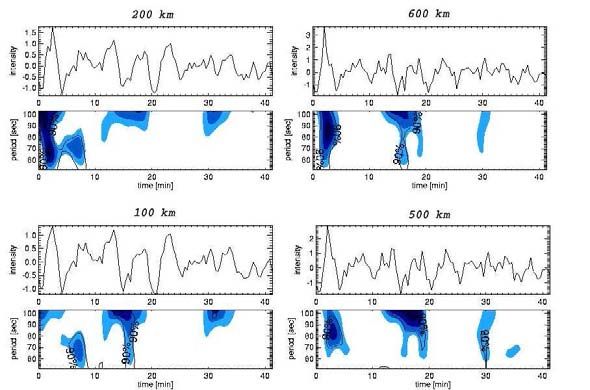
different heights. Fig. 4.1 represents my result of the wavelet analysis of fluctuations at
the same height (i.e.,( km) as the one used in (Wunnenberg et al. 2003).
Figure 4.1: Wavelet power section from data set DS2, calculated for the pixel I¿:( jKJ
in the image plane. The maximum of the heights which contribute to the observed
¹
fluctuations is at ( km.
394 Results
¹
Figure 4.2: Same as Fig 4.1 but for km height.
At the top row of the figures the velocity fluctuations are shown, and at the bottom
row the power of the short-period waves, both as function of time. Darker colour means
that large power is registered, light colour means that less power is registered. There are
6 areas in the bottom row of Fig. 4.1 which represent the finally obtained power.
¹
Fig. 4.2 shows the result of the wavelet analysis at the height of km. Here, only
three areas show power.
Table 4.1: Overview of the power occurrence at the height km.
Occurrence of power in time
time[min] periods[s] time for maximum power[min] periods for max. [s]
0-5 65-110 0-1.5 100-110
13-17 60-110 14-15.5 69-89
37-43 56-110 41 68-73
In Table 4.1 one can see an overview of the power appearing in Fig. 4.2; Table 4.2
gives an overview of the power from Fig. 4.1. It is noticeable that although both images
represent the same pixel in the data set, the results of the power are not the same. At
the higher level one can notice more power features distributed in time and apparently
without connection to the lower level. On the other hand power at the lower level, km,
might be related to some of the features at the higher level, although the distribution of
power is slightly different in time and period.
Short-period waves are not often visible in the signal presented in the top row of the
figures, since longer-periods are overwhelming. In figures 4.3 and 4.4 however, a signal
is present.
The different data sets show that power of short-period oscillations (in the range of
( s to s) appear at different heights in the solar chromosphere. It is evident that the
power varies in time and appears with varying amplitudes. In addition, at km the
power peaks appear to be less frequent than at ( km.
404.1 Waves at different heights
Table 4.2: Overview of the power occurrence at the height ( km.
Occurrence of power in time
time[min] periods[s] time for maximum power [min] periods for max. [s]
0-5 90-110 0-2 100-110
14-18 60-110 15-16 77-90
20.5-23.5 56-91 21.5-22.5 54-69
28-32 69-110 29-30 90-107
35-37 100-110 - -
36-38 56-85 36.5-37.5 60-68
Figure 4.3: The Doppler velocity fluctuations from data set DS2, at the pixel I¿:( jLJÏ
in the image for the height of ( km. The solid line represents filtered velocity fluctu-
1
ations in the period range s, the dashed line represents non-filtered signals from
the top row of Fig. 4.1.
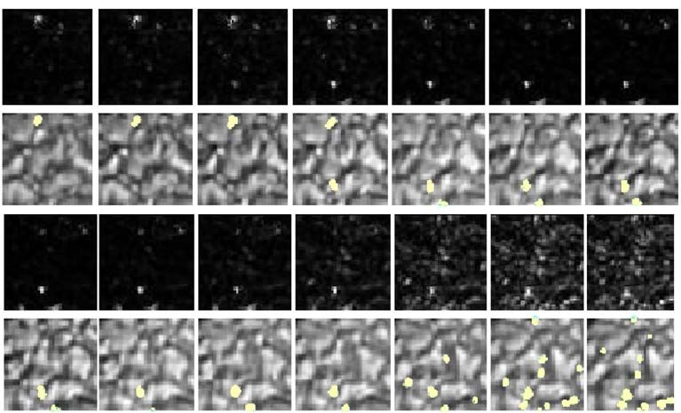
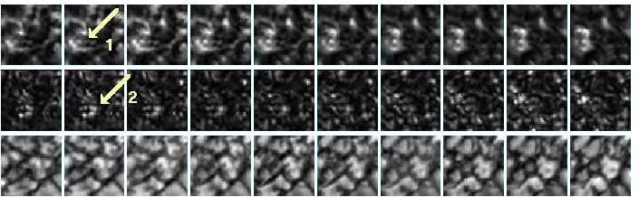
4.1.1 Spatial location
In Fig. 4.5 the power of short-period waves is shown as two-dimensional maps. It is
evident that power at the height km appears seldom in space as compared to power
at the height ( km, in agreement with the findings in figures 4.1 and 4.2. In the en-
larged rectangles one notices features which at km have low power and occur in three
different patches; at ( km these features are stronger in power and of different shape.
The power features at the height km which appear at the same location as the power
features at the height ( km tend to span less space. The shape of the power features
tends to vary with height. A possible explanation for this spatial variation is a character-
istic of short-period oscillations: they tend to expand in space while travelling upward.
The contribution to the spatial variation comes from the dissipation of waves of different
periods at different heights. The merging of waves from different sources additionally
complicates this picture.
An example of merging is shown in Fig. 4.6. In the top row it is seen that the power
features of the waves emitted from two neighbouring intergranular lanes merge into one
feature at ( km. This feature is marked with a green arrow at the beginning of its evo-
lution. The process is easier to see for waves with longer-periods since they change more
slowly in time (see section 4.5.1).
41You can also read