Correlation of core and downhole seismic velocities in high-pressure metamorphic rocks: a case study for the COSC-1 borehole, Sweden - GFZpublic

Page created by Jimmie Armstrong
 
CONTINUE READING
Correlation of core and downhole seismic velocities in high-pressure metamorphic rocks: a case study for the COSC-1 borehole, Sweden - GFZpublic
Solid Earth, 11, 607–626, 2020
https://doi.org/10.5194/se-11-607-2020
© Author(s) 2020. This work is distributed under
the Creative Commons Attribution 4.0 License.

Correlation of core and downhole seismic velocities in high-pressure
metamorphic rocks: a case study for the COSC-1 borehole, Sweden
Felix Kästner1,2 , Simona Pierdominici1 , Judith Elger2 , Alba Zappone3 , Jochem Kück1 , and Christian Berndt2
1 HelmholtzCentre Potsdam, GFZ German Research Centre for Geosciences, 14473 Potsdam, Germany
2 GEOMAR    Helmholtz Centre for Ocean Research Kiel, 24148 Kiel, Germany
3 Department of Earth Sciences, ETH Zurich, 8092 Zurich, Switzerland

Correspondence: Felix Kästner (felix.kaestner@gfz-potsdam.de)

Received: 18 October 2019 – Discussion started: 5 November 2019
Revised: 3 March 2020 – Accepted: 11 March 2020 – Published: 23 April 2020

Abstract. Deeply rooted thrust zones are key features of         those repeatedly occurring in the Himalayas (e.g., in 2015,
tectonic processes and the evolution of mountain belts. Ex-      M = 7.9, and 2008, M = 7.9), which are a potential threat
humed and deeply eroded orogens like the Scandinavian            to the local population. Their investigation, therefore, is im-
Caledonides allow us to study such systems from the surface.     portant to improve our understanding of the deeper orogenic
Previous seismic investigations of the Seve Nappe Complex        processes and tectonic evolution.
have shown indications of a strong but discontinuous reflec-        However, such structures are seldom directly accessible
tivity of this thrust zone, which is only poorly understood.     and difficult to image. An exception are exhumed systems
The correlation of seismic properties measured on borehole       where most parts of the orogen were deeply eroded and
cores with surface seismic data can constrain the origin of      exposed to upper crustal levels. The Caledonides of west-
this reflectivity. To this end, we compare seismic velocities    ern Scandinavia, a remnant of the mid-Paleozoic Caledonian
measured on cores to in situ velocities measured in the bore-    orogeny (e.g., Gee and Sturt, 1985), represent such a system.
hole. For some intervals of the COSC-1 borehole, the core        Here, available geophysical investigations of an orogen root
and downhole velocities deviate by up to 2 km s−1 . These dif-   can be compared to geological and petrophysical observa-
ferences in the core and downhole velocities are most likely     tions from the surface (e.g., Ebbing et al., 2012). Reflection
the result of microcracks mainly due to depressurization.        seismic data provide another possibility to investigate these
However, the core and downhole velocities of the intervals       thrust zones and revealed structures of a strong and highly
with mafic rocks are generally in close agreement. Seismic       diffuse reflectivity as, for example, observed at the highly
anisotropy measured in laboratory samples increases from         metamorphic Seve Nappe Complex in the Jämtland region,
about 5 % to 26 % at depth, correlating with a transition from   in central Sweden (e.g., Hedin et al., 2012).
gneissic to schistose foliation. Thus, metamorphic foliation        To better understand the origin of these reflections, one can
has a clear expression in seismic anisotropy. These results      compare them to the physical properties of the related rocks
will aid in the evaluation of core-derived seismic properties    at depths to characterize the impact of structural and compo-
of high-grade metamorphic rocks at the COSC-1 borehole           sitional variations on seismic properties. This involves com-
and elsewhere.                                                   parison of seismic velocities from different measurements
                                                                 and scales with both lithological and structural characteris-
                                                                 tics of cored rocks.
                                                                    In this study, we determine seismic properties on core
1   Introduction                                                 scale (millimeter to centimeter) from the COSC-1 borehole
                                                                 in western Jämtland, central Sweden (Fig. 1) and evaluate
Thrust zones in high-pressure metamorphic rocks are impor-       their potential to explain the in situ seismic properties (mil-
tant features in mountain belts. In active fault zones they      limeter to kilometer scale) by comparing core velocities with
are often accompanied by devastating earthquakes, such as

Published by Copernicus Publications on behalf of the European Geosciences Union.
Correlation of core and downhole seismic velocities in high-pressure metamorphic rocks: a case study for the COSC-1 borehole, Sweden - GFZpublic
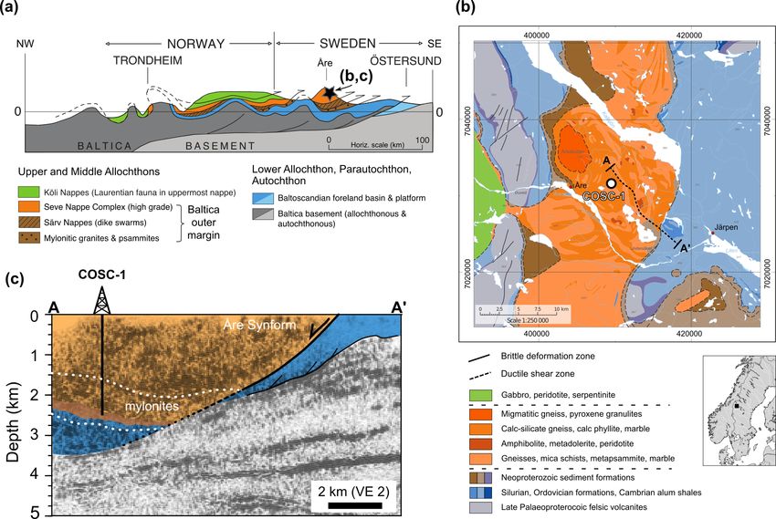
608                                                                                 F. Kästner et al.: Core–log seismic properties

Figure 1. Overview of the regional setting and study area. (a) Tectonostratigraphic division of the central Scandinavian Caledonides (Gee
et al., 2010; Lorenz et al., 2015a); (b) bedrock map with location of the COSC-1 borehole (colors modified; SGU Map Service; Strömberg
et al., 1994); (c) seismic cross section indicated in (b) showing a part of the COSC seismic profile (Hedin et al., 2012) with the COSC-1
borehole penetrating the highly reflective Lower Seve Nappe (adapted from Juhlin et al., 2016).

downhole logging data (centimeter to meter scale) and core             et al., 2002), where it was successfully used to better char-
lithology. Moreover, we focus on the effects of different am-          acterize the subsurface seismic stratigraphy using both core
bient pressure conditions on the velocities, the potential im-         and downhole logging data. But to date, there are only few
pact of microcracks and fracturing as well as scale differ-            studies that have adapted this concept in hard-rock environ-
ences inherent in the individual data sets and measurement             ments and similar metamorphic complexes. Some examples
procedures (Fig. 2).                                                   are the KTB borehole in Germany (Kern et al., 1991), the
   As core velocities measured under atmospheric pressure              Kola super-deep borehole in Russia (Golovataya et al., 2006),
conditions can exhibit strong deviations from in situ condi-           the Chinese Continental Scientific Drilling borehole in China
tions (Elbra et al., 2011), we integrate and compare the core          (Sun et al., 2012), and the Outokumpu deep drilling borehole
and downhole seismic velocities with laboratory velocity and           in Finland (Kukkonen, 2011).
anisotropy results from 16 core samples measured under dif-               The project COSC (Collisional Orogeny in the Scandina-
ferent confining pressure to simulate in situ conditions. Ul-          vian Caledonides) is a scientific drilling project co-funded
timately, this results in better constrained seismic properties        by the International Continental Scientific Drilling Program
in the vicinity of the COSC-1 borehole, which is a prerequi-           (ICDP), the Swedish Research Council, and the Geological
site for a successful core–log–seismic data integration (Wor-          Survey of Sweden. It generally aims to study the mountain
thington, 1994).                                                       building processes of the Scandinavian Caledonides in Swe-
   The concept of integration and cross-calibration of data            den (Gee et al., 2010; Lorenz et al., 2015a). In 2014, the
sets across different scales is well established in sedimentary        COSC-1 borehole was drilled in Åre, Jämtland (Fig. 1) to a
basins of marine and lake environments (e.g., Bloomer and              total depth of 2495.8 m. It was fully cored below 103 m with
Mayer, 1997; Miller et al., 2013; Riedel et al., 2013; Thu             almost 100 % core recovery. Drilling was accompanied by

Solid Earth, 11, 607–626, 2020                                                                    www.solid-earth.net/11/607/2020/
Correlation of core and downhole seismic velocities in high-pressure metamorphic rocks: a case study for the COSC-1 borehole, Sweden - GFZpublic
F. Kästner et al.: Core–log seismic properties                                                                                     609

Figure 2. Schematic depicting the different environmental and measurement conditions of the core, log, and borehole seismic (VSP) P-wave
velocity (Vp) measurement. Arrows indicate the direction of seismic wave propagation.

extensive field campaigns providing physical properties from          mostly composed of metasediments and carbonates from the
downhole logs and seismic profiles (Hedin et al., 2014, 2016;         Laurentian margin (Gee et al., 2008).
Krauß et al., 2015; Lorenz et al., 2015a; Simon et al., 2015).            The dimension of the Caledonian mountain range and its
Together with the excellent core recovery and data availabil-         formation mechanisms are similar to those of the more re-
ity, the COSC-1 drilling project constitutes a perfect case           cently formed Himalayan orogen (Labrousse et al., 2010).
study to apply core–log–seismic data integration in a meta-           Subsequent glaciation, tectonic uplift, and gravitational col-
morphic environment.                                                  lapse left most parts of the mountain range deeply eroded ex-
                                                                      posing rock formations of middle to lower crust levels (Gee
1.1   Geological background                                           et al., 2008). Today’s remnants, the Scandes, extend over a
                                                                      distance of about 300 km across the Scandinavian Peninsula,
In the mid-Paleozoic, the Caledonian orogen formed during             over a length of about 1700 km, from the Norwegian Skager-
the continent–continent collision of Laurentia and Baltica            rak coast in the south up to the North Cape. An extensive
(Gee et al., 2008). The Scandinavian Caledonides are com-             review of the Caledonian Orogeny and related areas is pro-
posed of nappes that were thrusted over the Baltic plat-              vided by Corfu et al. (2014) and Gee and Sturt (1985).
form margin accommodating several hundred kilometers of                   Along the COSC-1 borehole, based on the lithological de-
southeastward shortening. These thrust sheets are subdivided          scriptions of the cored rocks, four main sections were iden-
into the Lower, Middle, Upper, and Uppermost Allochthons,             tified at depth (Lorenz et al., 2015a): (1) gneisses of vary-
which rest on autochthonous crystalline basement (Fig. 1;             ing compositions (mainly felsic, amphibolitic, calc-silicate),
Gee et al., 2008; Roberts and Gee, 1985). The Lower Al-               often garnet- and diopside-bearing, occur from the top to
lochthon is mainly composed of sedimentary rocks of Up-               about 1800 m; (2) an extensive (ductile shear) deformation
per Proterozoic to Silurian age derived from the outer Bal-           zone prevails between 1800 and 2345 m; followed by (3) a
toscandian margin (Gee et al., 2010). The Middle Allochthon           15 m thick retrograde transition zone from amphibolite fa-
consists of several nappes with an increase in metamorphic            cies gneisses into lower-grade meta-sedimentary rocks; and
grade, derived from the outer to outermost Baltoscandian              (4) mylonitized quartzites and metasandstones of unclear
margin including the continent–ocean transition zone (Gee             tectonostratigraphic position that characterize the lowermost
et al., 2013). The uppermost part of the Middle Allochthon            part to the bottom of the borehole at 2495 m.
comprises the Seve Nappe Complex (SNC). The SNC is di-                    The potential to investigate the deep structure of the oro-
vided into a lower part of similar protolith to the underlying        genic root from the surface is directly addressed in the COSC
(greenschist facies) Särv Nappes but is highly deformed in            project. It generally focuses on the physical properties and
amphibolite and locally eclogite facies; a central part com-          inner structure of the emplaced nappe complex associated
posed of granulite facies migmatites and paragneisses (e.g.,          with high-grade metamorphic allochthonous rocks as well as
Ladenberger et al., 2014), overlaid by an upper part of lower-        the character and age of deformation of the underlying thrust
metamorphosed sedimentary rocks (Gee et al., 2010). The               sheets, the main Caledonian decollement, and the Precam-
Upper Allochthon is dominated by Early Paleozoic Iapetus-             brian basement (Gee et al., 2010; Lorenz et al., 2015a).
derived sedimentary rocks, ophiolites, and volcanic arc com-
plexes of greenschist facies. The Uppermost Allochthon is

www.solid-earth.net/11/607/2020/                                                                     Solid Earth, 11, 607–626, 2020
Correlation of core and downhole seismic velocities in high-pressure metamorphic rocks: a case study for the COSC-1 borehole, Sweden - GFZpublic
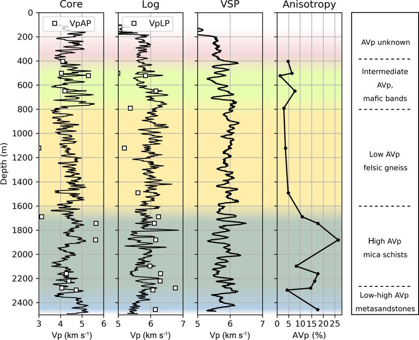
610                                                                             F. Kästner et al.: Core–log seismic properties

2     Data and methods                                             a good coupling with the signal transducers. The plugs were
                                                                   oven-dried at 100 ◦ C for at least 24 h in order to eliminate
For this study, we used compressional wave velocities from a       free water from the pore space.
multi-sensor core log (MSCL) and downhole data including              The plug dimensions (length and diameter) and dry weight
a short-spacing sonic log (Lorenz et al., 2015b) and zero-         were determined using a micrometer caliper (±0.01 mm) and
offset vertical seismic profile (Krauß et al., 2015) from the      precision balance (±1 mg), respectively. We used the aver-
COSC-1 borehole (see also Fig. 2). In addition, we measured        age diameter and length of four successive readings to re-
selected core samples to provide seismic properties of char-       duce possible errors due to surface irregularities. The ma-
acteristic lithological units. Based on these laboratory mea-      trix density of each core plug was measured using a He-
surements, we calculated velocities at different environmen-       gas pycnometer (type: AccuPyc II 1340). This is based on
tal conditions (intrinsic, lithostatic pressure, and atmospheric   a precise volume measurement using the gas displacement
pressure), which then served as a calibration tool for the core    method (Lowell et al., 2004, p. 326).
and downhole logging data. The individual data sets and ex-           The experimental procedure was similar to the one de-
perimental acquisition used for this study are described in        scribed in Wenning et al. (2016). For each core plug, ultra-
the following subsections. Table 1 provides an overview of         sonic seismic velocities were acquired under different con-
the individual measurements and related velocities and which       fining pressure using a hydrostatic pressure vessel and cor-
nomenclature is used throughout this study.                        responding acquisition system (Fig. 3; Barblan, 1990). The
                                                                   setup consisted of two piezoelectric transducers (lead–zircon
2.1    Laboratory measurements                                     ceramics, 1 MHz resonance frequency), transmitter, and re-
                                                                   ceiver, which were placed on the core plug’s cylinder faces.
Laboratory analyses are routinely applied to study the elas-       They were held in place by a shrink tube jacketing plug and
tic properties, fabric, and seismic anisotropy of crustal and      transducers. Additional metal wires, tightly wrapped around
mantle rocks (e.g., Barberini et al., 2007; Kern, 1982; Sieges-    the shrink tube, sealed the core plug to prevent any oil leak-
mund et al., 1991; Zappone et al., 2000). We used seismic          age into it (Fig. 3). The prepared core plug was mounted in-
wave velocities measured in 16 core samples. These mea-            side the vessel where the oil pressure was applied and con-
surements were conducted at room temperature and vary-             trolled using a pneumatic compressor. The pressure was first
ing confining pressure using the pulse-transmission method         increased in 50 MPa steps, from 50 to 250 MPa, and then de-
(Birch, 1960, 1961). In order to determine the seismic             creased in 30 MPa steps, between 240 and 30 MPa (±2 MPa).
anisotropy, i.e., the directional dependence of seismic veloc-     At each pressure step, a wave generator connected to one of
ity compressional (P) wave, the velocities were measured in        the transducers produced an input square signal 0.2 µs wide,
three mutually perpendicular core plugs drilled out of each        with an amplitude of 30 V, and a pulse rate of 0.5 kHz. Si-
of the 16 core samples.                                            multaneously, the wave generator sent a trigger signal with
   Six of these samples were measured by Wenning et                the same frequency to a PC-based wave analyzer. The ana-
al. (2016), chosen based on the most abundant lithologies          lyzer used an impedance of 1 M over a range of ±500 mV.
derived from the lithological core description (Lorenz et          The waveforms were recorded with a repetition rate of 80 ns
al., 2015b). In order to extend and complement these mea-          and a sampling rate of 100 MHz. The electric noise was min-
surements, we selected 10 additional samples at depth inter-       imized by averaging the tracks.
vals and lithologies that were not previously covered (see Ta-        The measurements were calibrated using steel cylinders of
ble A1 for a detailed sample list). In general, the 16 samples     varying lengths to correct for the delay in the observed travel
cover a large depth range of the borehole including potential      times (i.e., tobserved = trock +tsystem ), which was caused by the
zones of both higher and lower reflectivity as, for example,       cables, transducers, and interfaces in the electronic system.
indicated by the zero-offset vertical seismic profile (Krauß et    The calibration was conducted at confining pressures of 50
al., 2015).                                                        and 100 MPa. The system travel time (tsystem ) was obtained
   The core samples were cut at lengths of about 15 to 20 cm       by averaging the results from these two pressures.
from the COSC-1 drill cores. From each sample, we drilled             We performed our measurements at room temperature (ca.
three cylindrical core plugs of 3 to 5 cm length and 2.54 cm       22 ◦ C), which should be a good approximation of the in
diameter (see also Fig. 2). The orientation of the plug axes x,    situ condition because of the very low geothermal gradient
y, and z agree with the major structural axes that are defined     (ca. 20 ◦ C km−1 ) and low temperatures observed at about
by the sample’s foliation and lineation and which we have de-      2500 m, the bottom of the borehole (Tlog < 60 ◦ C; Lorenz et
termined by visual inspection. Following the common prac-          al., 2015b). Generally, seismic velocities decrease with tem-
tice (Zappone et al., 2000), we designated z as the axis nor-      perature (e.g., Motra and Stutz, 2018; Schön, 1996). How-
mal to the foliation plane. The foliation plane is spanned by      ever, at very low temperatures (< 100 ◦ C), like we observe
the x and y axes, where x is oriented parallel and y perpen-       in the COSC-1 borehole, this effect can be neglected (Kern,
dicular to the apparent lineation. The core plug ends were         1978). Moreover, the measured pressure-to-temperature in-
cut and ground to plane-parallel surfaces in order to provide      crement (about 1.5 MPa K−1 ) in the COSC-1 borehole is suf-

Solid Earth, 11, 607–626, 2020                                                                www.solid-earth.net/11/607/2020/
Correlation of core and downhole seismic velocities in high-pressure metamorphic rocks: a case study for the COSC-1 borehole, Sweden - GFZpublic
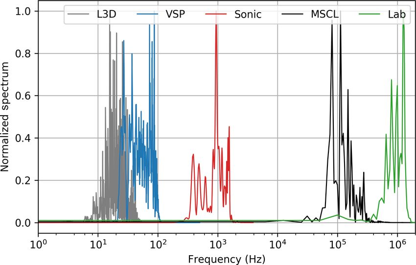
F. Kästner et al.: Core–log seismic properties                                                                                          611

Table 1. Overview of velocity nomenclature used in this study. The laboratory measurements were carried out on three mutually perpendicular
core plugs. See text for details.

     Velocity    Type of              Direction of           Description
                 measurement          measurement
     Vp0         Lab                  Triaxial               Intrinsic P-wave velocity based on laboratory measurements on core plugs
     VpAP        Lab                  Triaxial               P-wave velocity calculated at atmospheric pressure (p = 0.1 MPa)
                                                             based on laboratory measurements on core plugs
     VpLP        Lab                  Triaxial               P-wave velocity calculated at lithostatic pressure (p = Sv(z))
                                                             based on laboratory measurements on core plugs
     Core Vp     MSCL                 Perpendicular to       P-wave velocity continuously measured in whole cores using
                                      core axis              a multi-sensor core logger
     Log Vp      Downhole sonic       Parallel to borehole   P-wave velocity continuously logged downhole using a short-spacing
                                      axis                   sonic sonde (Lorenz et al., 2015b)
     VSP Vp      Borehole seismic     Parallel to borehole   P-wave velocities measured downhole using a zero-offset vertical
                                      axis                   seismic profile (Krauß et al., 2015)

                                                                           ply any additional filtering to the waveform data. First-arrival
                                                                           times were picked manually using a picking tool developed
                                                                           for this purpose (Grab et al., 2015). The seismic velocities
                                                                           were calculated using the plug length L, divided
                                                                                                                              by the cor-
                                                                           rected travel time: v = L/ tpicked − tsystem . Changes in the
                                                                           plug length due to compression can be neglected for these
                                                                           rock types (Zappone et al., 2000).
                                                                              We calculated P-wave velocities at atmospheric and at
                                                                           lithostatic pressure to relate to the different conditions of
                                                                           the velocity measurements from downhole sonic, MSCL, and
                                                                           borehole seismic data. The lithostatic pressure was calculated
                                                                           from the core and downhole logging density and is shown to-
                                                                           gether for the associated sample depths in Fig. 4. Since den-
                                                                           sity was only logged down to about 1600 m, we used extrapo-
                                                                           lated densities down to 2500 m depth showing slightly higher
                                                                           pressures than those calculated from the core.
                                                                              We used the relationship derived by Ji et al. (2007) to cal-
                                                                           culate P-wave velocity–pressure curves (Fig. 5) for each core
                                                                           plug of our 10 core samples. This relationship consisted of a
                                                                           four-parameter exponential equation to relate the measured
                                                                           velocities to confining pressure by solving a least-squares
Figure 3. Schematic of the experimental setup used to determine the        curve-fitting problem (Fig. 5). The intrinsic velocity (Vp0),
P-wave velocities under confining pressure. This setup comprises a         which corresponds to the undisturbed, crack-free rock ma-
pressure vessel with a sample chamber, pulse generator, compressor         trix, was calculated from the intercept of the extrapolated
control, and PC-based acquisition unit. Placed inside the oil-filled       linear part of the velocity–pressure relation. The velocities
pressure chamber there is the sample assembly (based on Barblan,           at room pressure (VpAP, p = 0.1 MPa) and lithostatic pres-
1990).                                                                     sure (VpLP, p = Sv) were determined from the non-linear
                                                                           representation of the velocity–pressure relation (Fig. 5).
                                                                              Wenning et al. (2016) used a slightly different relation
ficiently high to prevent thermal microcracking (see Kern,                 for their six samples, proposed by Wepfer and Christensen
1990).                                                                     (1991). For most applications aiming to determine the lin-
   In the subsequent data processing, we calculated velocities             ear high-pressure part and intrinsic anisotropy, both relations
and anisotropy coefficients as a function of confining pres-               give consistent results. However, the inherent zero-boundary
sure for each core plug and sample, respectively. Because                  condition of Wepfer and Christensen’s relation may lead to
of a very good signal quality, it was not necessary to ap-

www.solid-earth.net/11/607/2020/                                                                         Solid Earth, 11, 607–626, 2020
Correlation of core and downhole seismic velocities in high-pressure metamorphic rocks: a case study for the COSC-1 borehole, Sweden - GFZpublic
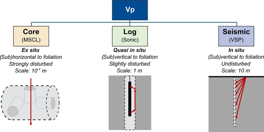
612                                                                                   F. Kästner et al.: Core–log seismic properties

                                                                         of the velocity anisotropy (Birch, 1961; Crampin, 1989;
                                                                         Schön, 1996). These representations are generally based on
                                                                         a fractional difference of the maximum and minimum mea-
                                                                         sured velocities but distinguished in the applied denomina-
                                                                         tor. We used a definition after Crampin (1989), which is
                                                                         described by the degree of the fractional difference of the
                                                                         maximum and minimum velocity of the rock sample; i.e.,
                                                                         AVp = 100 × (Vpmax − Vpmin )/Vpmax .
                                                                            The main source of error in the determination of seis-
                                                                         mic velocity is the uncertainty in picking the first-arrival
                                                                         times. We estimated a typical uncertainty in the picking of
                                                                         the P-wave first arrivals with an upper limit of δtobserved ∼
                                                                                                                                     =
                                                                         ±0.1 µs. The seismic velocity uncertainty was estimated us-
                                                                         ing the concept of error propagation (e.g., Taylor, 1997),
Figure 4. Lithostatic pressure curve of the COSC-1 borehole de-          providing a measured P-wave velocity uncertainty of δVp =
rived from core and downhole density measurements (Lorenz et             ±0.11 km s−1 on average. The uncertainty propagation in the
al., 2015b). The values for the 16 core samples are marked accord-       extrapolated velocities at zero confining pressure (δVp0) was
ingly. The dashed line was linearly extrapolated since downhole          based on the linear regression function that minimized the
density was only logged down to about 1.6 km.                            sum of the squared errors of the prediction. Subsequently, we
                                                                         used the error of the regression coefficients (i.e., slope and
                                                                         intercept) to derive the uncertainty for the anisotropy coeffi-
                                                                         cient (AVp) using the same approach as for the measured ve-
                                                                         locities. The uncertainty of the P-wave anisotropy was below
                                                                         1 % for all samples. Moreover, our error analysis has shown
                                                                         that the bulk uncertainty of the measured seismic velocities
                                                                         is dominated by the pick accuracy of the pulse arrival picks,
                                                                         while errors in the plug length only have a minor impact.

                                                                         2.2   Multi-sensor core log P-wave velocity

                                                                         Seismic P-wave velocity was measured every 5 cm on the
                                                                         2.5 km COSC-1 cores using an MSCL (type Geotek MSCL-
                                                                         S), which is based on an automated full-waveform logging
                                                                         system (e.g., Breitzke and Spieß, 1993; Weber et al., 1997).
                                                                         The P-wave sensor setup comprised two signal transducers
Figure 5. Schematic velocity–pressure relation depicting the mea-
                                                                         mounted on opposite sides, perpendicular to the core axis.
sured and calculated seismic P-wave velocity Vp as a function of
confining pressure p. Based on the best curve fit for the linear
                                                                         The upper one was a motor-driven piston transmitter, while
(dashed line) and non-linear part (solid line), velocities can be cal-   the lower one used a spring-loaded acoustic rolling contact
culated under different environmental conditions: Vp0 – intrinsic        (ARC), constantly pushed against the measured cores.
velocity, VpAP – atmospheric pressure, VpLP – lithostatic pressure          At each measuring position, a 230 kHz P-wave pulse was
(adapted from Ji et al., 2007).                                          sent from the transmitter through the core and was recorded
                                                                         by the receiver. The recorded signal was pre-amplified, digi-
                                                                         tized, and sent to the acquisition software at a sampling fre-
underestimated velocities in the extrapolated, non-linear low-           quency of 12.5 MHz. The first-arrival times were determined
pressure part, which is why we used the relationship by Ji et            using a threshold method providing a user-defined threshold
al. (2007) for our 10 samples, instead.                                  level and time delay. This system automatically determined
   A full data example for one sample is shown in Fig. 6. It             the first excursion above the given threshold, after the delay.
shows the measured P-wave velocities as a function of in-                The total travel time (TOT) was then taken at the first zero-
creasing and decreasing confining pressure for each of the               crossing. During the acquisition procedure, the voltage level
three core plugs and the velocity–pressure curves calculated             (amplitude), threshold level, and time delay were adjusted
from the downgoing pressure cycles.                                      automatically, to ensure a good signal-to-noise ratio for the
   The intrinsic seismic anisotropy (AVp) was determined                 automatic picker. To provide a good coupling between the
from the Vp0 measured along the x, y, and z directions                   transducers and the core, the core surface was wetted before
(Fig. 6). In the literature there are different representations          the measurement.

Solid Earth, 11, 607–626, 2020                                                                     www.solid-earth.net/11/607/2020/
F. Kästner et al.: Core–log seismic properties                                                                                             613

Figure 6. Data example showing confining pressure versus P-wave velocity (Vp) and anisotropy (AVp) for sample 569-2 (see Table 2). Open
symbols refer to measurements during pressurization and filled symbols to measurements during depressurization. Different markers indicate
the velocities measured in the respective x, y, and z core plugs along the corresponding structural axes (see also Fig. 5 and text for details).

   Furthermore, a calibration was carried out to determine the
P-wave travel time offset (PTO), which accounts for the ac-
cumulated travel time delays through the transducer system
(transducer faces, rubber plates, etc.). The actual travel time
(TT) was derived by subtracting the PTO from total mea-
sured travel time, i.e., TT = TOT − PTO.
   The calibration based on travel times measured in whole-
round and half-split POM (polyoxymethylen) cylinders of
varying diameters (60 to 120 mm), which were plotted and
extrapolated by a best linear fit. The P-wave velocities
were calculated using the corrected travel time TT and the
nominal core diameter (D = 61 and 47.6 mm), by Vp =
D/ (TOT − PTO) = D/TT. No additional temperature cor-
rection was applied because the room temperature inside the
laboratory was kept constant at about 21 ◦ C.                             Figure 7. Comparison of frequency spectra of seismic measure-
                                                                          ments across multiple scales from limited 3D surface seismic
                                                                          (L3D), borehole seismic (VSP), downhole log (sonic), core mea-
2.3   Downhole sonic logging
                                                                          surement (MSCL), and laboratory samples (Lab). The downhole-
                                                                          related spectra are calculated from a single seismic trace and sonic
A downhole sonic measurement was carried out as part                      waveform extracted from approximately the same downhole depth
of a complete downhole logging campaign in 2014, about                    of about 500 m.
1 month after the drilling of the COSC-1 borehole was
completed. The original data set is published by Lorenz et
al. (2015b, 2019) and comprises, amongst other things, a
density log and 3D core scan images. Downhole sonic ve-
locities were continuously logged every 0.1 m by the Oper-
ational Support Group (OSG) of the ICDP using a standard
full-waveform slimhole sonde (Antares, Germany). Transit                  on the formation velocities and frequencies and can be es-
times were calculated from first-arrival times, which first               timated by 3 times the dominant wavelength (Serra, 1984).
were picked automatically and then refined manually. The                  The frequency range of the recorded sonic traces lies in the
seismic P-wave velocities were calculated using the sonde’s               order of a few kilohertz (Fig. 7). For the given sonde geome-
receiver spacing (0.5 m) divided by the transit time.                     try and nominal transmitter frequency (20 kHz), the depth of
   Based on refracted waves propagating along the borehole                investigation is about 0.75 to 1 m. Thus, downhole logging
wall, the sonic log represents a vertical average velocity of             velocities provide a good approximation of the in situ seis-
the near-well vicinity over the receiver spacing. The inves-              mic velocities but can still be affected by micro-fracturing
tigation depth and resolved rock volume generally depend                  caused by drilling or steeply dipping natural fractures.

www.solid-earth.net/11/607/2020/                                                                           Solid Earth, 11, 607–626, 2020
614                                                                                                                                                             F. Kästner et al.: Core–log seismic properties

2.4    Zero-offset vertical seismic profile

                                                                   ∗ Samples measured by Wenning et al. (2016); AVp data recalculated. NA: not available.

                                                                                                                                                                                                                                       Table 2. Laboratory data of 16 rock samples from the COSC-1 borehole. Sv – Lithostatic pressure derived from core density.
                                                                                                                                                            691-1∗
                                                                                                                                                            664-2
                                                                                                                                                            661-3
                                                                                                                                                            651-5
                                                                                                                                                            641-5
                                                                                                                                                            631-1∗
                                                                                                                                                            593-4
                                                                                                                                                            569-2
                                                                                                                                                            556-2∗
                                                                                                                                                            487-1∗
                                                                                                                                                            361-2
                                                                                                                                                            243-2∗
                                                                                                                                                            193-2∗
                                                                                                                                                            149-4
                                                                                                                                                            143-1
                                                                                                                                                            106-1

                                                                                                                                                                                                                      Sample
A zero-offset vertical seismic profile (VSP) was acquired
in the COSC-1 borehole, as part of a comprehensive post-

                                                                                                                                                            Grt-bearing mica schist
                                                                                                                                                            Metasandstone
                                                                                                                                                            Am-rich gneiss (mylonite)
                                                                                                                                                            Mica schist (mylonite)
                                                                                                                                                            Mica schist
                                                                                                                                                            Am-rich gneiss
                                                                                                                                                            Paragneiss
                                                                                                                                                            Mica schist
                                                                                                                                                            Amphibolite
                                                                                                                                                            Felsic gneiss
                                                                                                                                                            Gneiss
                                                                                                                                                            Calc-silicate gneiss
                                                                                                                                                            Amphibolite
                                                                                                                                                            Metagabbro
                                                                                                                                                            Gneiss
                                                                                                                                                            Migmatite

                                                                                                                                                                                                                      Core Lithology
drilling seismic survey to image the SNC and its underlying
formations (Krauß, 2017; Krauß et al., 2015). In our study,
we used the P-wave velocities that were calculated by the
first-arrival times of the consecutive downhole receiver sta-
tions. The receiver spacing was 2 m and the first-arrival times
were smoothed by a 15-point moving average (30 m interval)
to account for small travel time variations.
   For a zero-offset (or rig-source) borehole seismic, the di-

                                                                                                                                                            2457.26
                                                                                                                                                            2296.29
                                                                                                                                                            2279.31
                                                                                                                                                            2220.52
                                                                                                                                                            2160.64
                                                                                                                                                            2097.65
                                                                                                                                                            1881.51
                                                                                                                                                            1744.27
                                                                                                                                                            1689.94
                                                                                                                                                            1491.72
                                                                                                                                                            1121.48
                                                                                                                                                             791.22
                                                                                                                                                             649.59
                                                                                                                                                             522.41
                                                                                                                                                             502.10
                                                                                                                                                             403.09

                                                                                                                                                                                                        Depth
rect P-wave ideally propagates downwards from the surface,

                                                                                                                                                                                                          (m)
parallel to the borehole. Thus, being relatively unaffected
by the borehole itself, borehole-seismic velocities provide a

                                                                                                                                                                                                        (g cm−3 )
                                                                                                                                                                                                         Density
                                                                                                                                                            2.85
                                                                                                                                                            2.68
                                                                                                                                                            2.94
                                                                                                                                                            2.77
                                                                                                                                                            2.81
                                                                                                                                                            3.07
                                                                                                                                                            2.83
                                                                                                                                                            2.83
                                                                                                                                                            3.09
                                                                                                                                                            2.81
                                                                                                                                                            2.71
                                                                                                                                                            2.75
                                                                                                                                                            3.08
                                                                                                                                                            2.99
                                                                                                                                                            2.73
                                                                                                                                                            2.76
good approximation of the vertical in situ seismic velocity of
the borehole vicinity. The calculated, so-called interval ve-
locity represents the constant velocity of the seismic wave

                                                                                                                                                                                                        (MPa)
                                                                                                                                                            66.17
                                                                                                                                                            61.97
                                                                                                                                                            61.53
                                                                                                                                                            59.97
                                                                                                                                                            58.53
                                                                                                                                                            56.87
                                                                                                                                                            51.18
                                                                                                                                                            47.55
                                                                                                                                                            46.08
                                                                                                                                                            40.63
                                                                                                                                                            30.61
                                                                                                                                                            21.59
                                                                                                                                                            17.58
                                                                                                                                                            14.13
                                                                                                                                                            13.56
                                                                                                                                                            10.83
traveling through a rock layer with a given interval thick-

                                                                                                                                                                                                         Sv
ness, which is defined by the applied receiver spacing (2 m).
Thus, the distance over which the velocity is averaged is 4

                                                                                                                                                            6.42
                                                                                                                                                            6.09
                                                                                                                                                            7.32
                                                                                                                                                            6.74
                                                                                                                                                            6.92
                                                                                                                                                            7.12
                                                                                                                                                            6.90
                                                                                                                                                            6.67
                                                                                                                                                            7.25
                                                                                                                                                            6.42
                                                                                                                                                            5.93
                                                                                                                                                            6.44
                                                                                                                                                            7.23
                                                                                                                                                            6.53
                                                                                                                                                            6.09
                                                                                                                                                            5.93
                                                                                                                                                                                                x
times larger than for the downhole sonic log (at 0.5 m re-

                                                                                                                                                                                                        Intrinsic velocity Vp0
ceiver spacing).                                                                                                                                            6.68
                                                                                                                                                            6.31
                                                                                                                                                            6.79
                                                                                                                                                            6.41
                                                                                                                                                            6.41
                                                                                                                                                            6.78
                                                                                                                                                            6.52
                                                                                                                                                            6.36
                                                                                                                                                            6.88
                                                                                                                                                            6.31
                                                                                                                                                            6.13
                                                                                                                                                            6.37
                                                                                                                                                            6.93
                                                                                                                                                            6.52
                                                                                                                                                            6.28
                                                                                                                                                            6.10
                                                                                                                                                                                                y
                                                                                                                                                                                                               (km s−1 )
   The signal frequencies ranged between 80 and 100 Hz
(Fig. 7). The measurement scale was mainly dictated by the
                                                                                                                                                            5.51
                                                                                                                                                            6.04
                                                                                                                                                            6.26
                                                                                                                                                            5.64
                                                                                                                                                            5.70
                                                                                                                                                            6.53
                                                                                                                                                            5.08
                                                                                                                                                            5.50
                                                                                                                                                            6.46
                                                                                                                                                            6.11
                                                                                                                                                            5.91
                                                                                                                                                            6.25
                                                                                                                                                            6.67
                                                                                                                                                            6.44
                                                                                                                                                            5.87
                                                                                                                                                            5.81
                                                                                                                                                                                                z
horizontal and vertical resolution. The former can be ap-
proximated by the first Fresnel zone of the dominant seismic

                                                                                                                                                                                                Mean
                                                                                                                                                            6.20
                                                                                                                                                            6.15
                                                                                                                                                            6.79
                                                                                                                                                            6.27
                                                                                                                                                            6.35
                                                                                                                                                            6.81
                                                                                                                                                            6.17
                                                                                                                                                            6.18
                                                                                                                                                            6.86
                                                                                                                                                            6.28
                                                                                                                                                            5.99
                                                                                                                                                            6.35
                                                                                                                                                            6.94
                                                                                                                                                            6.50
                                                                                                                                                            6.08
                                                                                                                                                            5.94
wavelength. For the COSC-1 borehole range (0 to 2500 m),
this yielded an average horizontal resolution of about 300 m
                                                                                                                                                            17.51

                                                                                                                                                            14.56
                                                                                                                                                            16.27
                                                                                                                                                            17.65

                                                                                                                                                            26.41
                                                                                                                                                            17.63
                                                                                                                                                            10.90

                                                                                                                                                                                                        Intrinsic anisotropy
(λ = 75 m, vconst. = 6 km s−1 ). In contrast, the vertical reso-

                                                                                                                                                                                                AVp
                                                                                                                                                             4.36

                                                                                                                                                             8.29

                                                                                                                                                             4.83
                                                                                                                                                             3.63
                                                                                                                                                             2.95
                                                                                                                                                             7.75
                                                                                                                                                             1.29
                                                                                                                                                             6.44
                                                                                                                                                             4.79
lution was about 20 m, assuming one-quarter of the dominant

                                                                                                                                                                                                                 (%)
wavelength (Rayleigh resolution limit).
                                                                                                                                                            NA
                                                                                                                                                            0.13
                                                                                                                                                            0.34
                                                                                                                                                            0.27
                                                                                                                                                            0.56
                                                                                                                                                            NA
                                                                                                                                                            0.17
                                                                                                                                                            0.18
                                                                                                                                                            NA
                                                                                                                                                            NA
                                                                                                                                                            0.92
                                                                                                                                                            NA
                                                                                                                                                            NA
                                                                                                                                                            0.67
                                                                                                                                                            0.62
                                                                                                                                                            0.35
                                                                                                                                                                                                Error
3     Results
                                                                                                                                                            2.45
                                                                                                                                                            4.68
                                                                                                                                                            2.74
                                                                                                                                                            5.58
                                                                                                                                                            4.37
                                                                                                                                                            3.22
                                                                                                                                                            6.50
                                                                                                                                                            6.12
                                                                                                                                                            4.73
                                                                                                                                                            1.66
                                                                                                                                                            3.18
                                                                                                                                                            1.50
                                                                                                                                                            4.33
                                                                                                                                                            6.38
                                                                                                                                                            3.91
                                                                                                                                                            4.08
                                                                                                                                                                                                x

                                                                                                                                                                                                        Extrinsic velocity VpAP
3.1    Laboratory data
                                                                                                                                                            3.69
                                                                                                                                                            5.07
                                                                                                                                                            5.94
                                                                                                                                                            5.08
                                                                                                                                                            4.93
                                                                                                                                                            2.13
                                                                                                                                                            6.08
                                                                                                                                                            5.94
                                                                                                                                                            2.65
                                                                                                                                                            1.40
                                                                                                                                                            3.43
                                                                                                                                                            2.40
                                                                                                                                                            4.03
                                                                                                                                                            5.83
                                                                                                                                                            4.51
                                                                                                                                                            4.45
                                                                                                                                                                                                y
                                                                                                                                                                                                                (km s−1 )

The laboratory intrinsic seismic velocities lie between 5.9
                                                                                                                                                            2.59
                                                                                                                                                            4.44
                                                                                                                                                            3.53
                                                                                                                                                            2.51
                                                                                                                                                            3.53
                                                                                                                                                            1.78
                                                                                                                                                            4.29
                                                                                                                                                            4.89
                                                                                                                                                            2.02
                                                                                                                                                            1.40
                                                                                                                                                            2.40
                                                                                                                                                            1.04
                                                                                                                                                            4.27
                                                                                                                                                            3.68
                                                                                                                                                            3.73
                                                                                                                                                            3.80

and 6.9 km s−1 showing generally little scattering (SD =
                                                                                                                                                                                                z

0.3 km s−1 ) throughout all samples (Table 2). The slowest
                                                                                                                                                                                                Mean
                                                                                                                                                            2.91
                                                                                                                                                            4.73
                                                                                                                                                            4.07
                                                                                                                                                            4.39
                                                                                                                                                            4.28
                                                                                                                                                            2.38
                                                                                                                                                            5.63
                                                                                                                                                            5.65
                                                                                                                                                            3.13
                                                                                                                                                            1.49
                                                                                                                                                            3.00
                                                                                                                                                            1.65
                                                                                                                                                            4.21
                                                                                                                                                            5.30
                                                                                                                                                            4.05
                                                                                                                                                            4.11

velocities occur always along the z axis, thus perpendicular
to the foliation plane. Highest velocities occur in the folia-
tion plane, i.e., along the x and y axes. The intrinsic seis-
                                                                                                                                                            6.41
                                                                                                                                                            6.06
                                                                                                                                                            7.35
                                                                                                                                                            6.76
                                                                                                                                                            6.98
                                                                                                                                                            6.27
                                                                                                                                                            6.89
                                                                                                                                                            6.60
                                                                                                                                                            6.81
                                                                                                                                                            5.75
                                                                                                                                                            5.18
                                                                                                                                                            5.40
                                                                                                                                                            6.42
                                                                                                                                                            6.44
                                                                                                                                                            4.94
                                                                                                                                                            4.72

                                                                                                                                                                                                        Lithostatic velocity VpLP
                                                                                                                                                                                                x

mic anisotropy exhibits a strong variation between 1 % and
26 %, with an average error of 0.4 %. The average seismic
                                                                                                                                                            6.54
                                                                                                                                                            6.22
                                                                                                                                                            6.73
                                                                                                                                                            6.46
                                                                                                                                                            6.36
                                                                                                                                                            6.04
                                                                                                                                                            6.47
                                                                                                                                                            6.32
                                                                                                                                                            6.36
                                                                                                                                                            5.65
                                                                                                                                                            5.44
                                                                                                                                                            5.55
                                                                                                                                                            6.13
                                                                                                                                                            6.06
                                                                                                                                                            5.28
                                                                                                                                                            5.05
                                                                                                                                                                                                y
                                                                                                                                                                                                                (km s−1 )

anisotropy for all 16 samples is about 10 % (Table 2).
   Velocities calculated at lithostatic pressure show val-
                                                                                                                                                            5.49
                                                                                                                                                            5.93
                                                                                                                                                            6.21
                                                                                                                                                            5.66
                                                                                                                                                            5.57
                                                                                                                                                            5.62
                                                                                                                                                            5.10
                                                                                                                                                            5.43
                                                                                                                                                            5.57
                                                                                                                                                            5.42
                                                                                                                                                            4.96
                                                                                                                                                            5.18
                                                                                                                                                            5.95
                                                                                                                                                            5.02
                                                                                                                                                            4.73
                                                                                                                                                            4.56
                                                                                                                                                                                                z

ues between 4.8 and 6.8 km s−1 (SD = 0.5 km s−1 ). Veloc-
ities calculated at atmospheric pressure are significantly
                                                                                                                                                                                                Mean
                                                                                                                                                            6.15
                                                                                                                                                            6.07
                                                                                                                                                            6.76
                                                                                                                                                            6.30
                                                                                                                                                            6.31
                                                                                                                                                            5.98
                                                                                                                                                            6.16
                                                                                                                                                            6.12
                                                                                                                                                            6.25
                                                                                                                                                            5.61
                                                                                                                                                            5.19
                                                                                                                                                            5.38
                                                                                                                                                            6.17
                                                                                                                                                            5.84
                                                                                                                                                            4.98
                                                                                                                                                            4.78

lower, ranging from 1.5 to 5.7 km s−1 on average (SD =
1.3 km s−1 ). The measured sample densities vary between
2.7 and 3.1 g cm−3 , with the highest densities observed for
the amphibole-rich (mafic) samples (149-4, 193-2, 556-2,
631-1, and 661-3).

Solid Earth, 11, 607–626, 2020                                                                                                                                             www.solid-earth.net/11/607/2020/
F. Kästner et al.: Core–log seismic properties                                                                                        615

Figure 8. Mean intrinsic velocity measured in 16 core samples          Figure 9. Seismic anisotropy measured in 16 rock samples from
from the COSC-1 borehole plotted at the respective sample depth.       the COSC-1 borehole plotted at the respective sample depth. Mark-
Markers correspond to simplified lithological classes such as mafic    ers correspond to simplified lithological classes such as mafic
amphibole-rich units (), felsic gneisses and metasandstone (•), and   amphibole-rich units (), felsic gneisses and metasandstone (•), and
mica schist (N). Note that the highest values occur for the mafic      mica schist (N).
lithologies.

   The mean intrinsic P-wave velocities (Vp0) were derived
from the three-axial (x, y, and z) core plug measurements (cf.
Fig. 6). These represent the most general case excluding any
directional or structural effects and mainly account for the
compositional effects (Fig. 8). Amphibole-rich (mafic) rock
samples have velocities ranging between 6.5 and 6.9 km s−1 ,
whereas all other more felsic rock samples including the fel-
sic gneisses, mica schists, and metasandstone, are character-
ized by a Vp0 between 6.0 and 6.4 km s−1 . The lowest Vp0
can be associated with the felsic gneiss samples, while the
mica-rich schists show slightly higher Vp0. Moreover, both
                                                                       Figure 10. Distribution of P-wave velocities derived from labo-
metasandstone (sample 664-2) and the carbonate-rich gneiss             ratory samples (Vp0, VpLP, VpAp), core measurements (Core),
(sample 243-2) show very similar Vp0 as for the mica schists           downhole logging (Log), and borehole seismic (VSP). The sample
(e.g., samples 641-5, 651-5).                                          velocities are displayed below the histograms indicating the mean
   The seismic P-wave anisotropy (AVp) changes with in-                and standard deviation of the 16 laboratory core samples.
creasing depth. This provides a simplified anisotropy–depth
profile along the COSC-1 borehole (Fig. 9). The uppermost
about 600 m show medium anisotropy (< 10 %) and low val-               3.2   Lab, core, and log data integration
ues (< 5 %) between 750 and 1500 m. Between 1600 and
1900 m, we observe the highest anisotropy effect with val-             Downhole sonic and VSP logs show a good correlation,
ues up to 25 %, which decreases again, further below.                  while VSP velocities have a lower resolution caused by the
   Comparing the different velocity distributions, the veloci-         averaging. The raw core velocities show a strong scattering
ties at atmospheric pressure (VpAP) show very strong scat-             and lower velocities on average (Fig. 10).
tering and generally low values, agreeing well with the ve-               As we generally relate the core-derived data to measure-
locities measured in core under similar pressure conditions            ments at surface conditions and the sonic and VSP logs to
(Fig. 10). Velocities at lithostatic pressure (VpLP), in con-          measurements under hydrostatic pressure in the borehole and
trast, follow the in situ velocities measured downhole by the          the in situ rock (cf. Fig. 2), we expect the downhole mea-
sonic and zero-offset VSP logs. On average, the intrinsic ve-          surements to show potentially higher velocities than those
locities (Vp0) are slightly higher than those calculated under         measured in core. Our data show that there is neither a clear
lithostatic pressure.                                                  correlation between core and downhole velocities nor an ob-

www.solid-earth.net/11/607/2020/                                                                      Solid Earth, 11, 607–626, 2020
616                                                                            F. Kästner et al.: Core–log seismic properties

servable static offset with depth (Fig. 11). There are places     samples. We cannot observe any direct correlation of the fo-
where the core-derived Vp increases, while the downhole-          liation dips and the velocity data.
measured Vp decreases, for example in the lowermost 200 m
of the borehole. Moreover, we can observe core velocities         3.3   Comparison of velocity data at core scale
that closely approach or even exceed the downhole velocities
(430 to 780; 1700 to 2000 m), while at other depth intervals      We conducted a detailed analysis of the measured seismic
(620, 1640, and 1800 m) core and downhole Vp mismatch             velocities at core scale (centimeter to millimeter), for six se-
significantly. Between 160 and 180 m, we see a strong de-         lected core sections (Fig. 12a–f), which represent character-
crease in downhole P-wave velocities, which are likely re-        istic lithological units with respect to their seismic proper-
lated to a karstic unit previously recognized by a very high      ties. We compared the measured core and downhole veloci-
secondary porosity (Lorenz et al., 2015b). Here, the core and     ties with the laboratory results and correlated them with the
downhole velocities show good agreement.                          unrolled 360◦ core scans (Lorenz et al., 2015b) of each se-
   From about 430 to 780 m, we observe several peaks in the       lected core section. Missing core data are caused by samples
core velocities, which also correlate with peaks in the down-     taken previously from the core measurements.
hole velocity and density logs. Between 780 and 1900 m               Section 106-1 (Fig. 12a) is a migmatite unit that is char-
the core velocities gradually increase and they are accompa-      acterized by an alteration of darker restite bands and leuco-
nied by several smaller, less pronounced peaks, which often       cratic melts (chemically very similar to felsic gneiss). Both
match with peaks in the downhole velocity and density logs        core and downhole velocities are relatively stable showing
(e.g., between 900 and 1000 m). From about 1900 m, down           an average difference of about 1.6 km s−1 . Sample velocities
to about 2350 m, the core velocities tend to decrease, before     calculated at atmospheric conditions agree with the very low
they increase again abruptly and clearly approach the down-       core Vp. The lithostatic velocity, however, is lower than those
hole velocities. Zones of clear opposite trends in the core ve-   logged downhole, whereas the intrinsic velocities are higher.
locities and downhole or VSP logs can be seen, for example,       This indicates a strong effect of microcracks with poor ori-
at 200 to 240, 600 to 625, 1200 to 1250, or 1625 to 1650 m.       entation. The intrinsic seismic anisotropy is comparably low
These intervals encompass various core lithologies but most       (< 5 %). Similar results were obtained for the gneiss sample
abundantly correlate with gneiss, calc-silicate rock, and am-     (e.g., sample 143-1; cf. Fig. 11), which have slightly higher
phibole gneiss.                                                   core velocities (ca. 4.5 km s−1 ) but similar downhole Vp (ca.
   In general, the superimposed mean sample velocities (in-       5.6 km s−1 ).
trinsic Vp0, atmospheric VpAP, and lithostatic VpLP) corre-          Section 193-2 (Fig. 12b) contains amphibolite where core
late well with the associated core (corresponds to VpAP) and      and downhole velocities match well. We observe similar re-
downhole (corresponds to VpLP and Vp0) velocities. The            sults for the metagabbro (sample 149-4, cf. Fig. 11), which
sample densities match almost perfectly the core and down-        are chemically almost equivalent. A fracture in the core sec-
hole density measurements. While the mean intrinsic veloc-        tion can be clearly identified by the core Vp. The velocities
ity Vp0 agree mostly with the downhole seismic velocities,        at lithostatic pressure match almost perfectly with the down-
they are slightly higher in some depth intervals (e.g., samples   hole velocity, whereas the velocities at atmospheric pressure
193-2, 631-1), possibly due to anisotropy effects. The mean       are considerably lower than the associated core velocities.
velocities calculated at lithostatic pressure (i.e., VpLP) are    In comparison with the amphibolite sections, the metagab-
generally consistent with the downhole velocities and only        bro exhibits only slightly higher downhole velocities, which,
show slightly lower values for samples 106-1, 143-1, 243-         however, still agree with velocities measured in core. In gen-
2, and 361-2, which are located above about 1600 m. Be-           eral, both units show very similar characteristics.
low about 1700 m, all samples (except sample 631-1) show             Section 361-2 (Fig. 12c) is dominated by gneiss of felsic
very similar VpLP to the intrinsic velocities Vp0 (cf. Fig. 11,   composition and shows similar characteristics as the upper-
where markers are partly overlapped).                             most gneiss sections (e.g., sample 143-1; cf. Fig. 11) and
   The velocities calculated at atmospheric pressure (i.e.,       slightly higher velocities, which possibly relates to an in-
VpAP) match the core velocities except for the samples 361-       crease in mafic minerals such as amphibole. The core and
2, 556-2, 631-1, and 691-1. For samples 243-2 and 487-1           downhole Vp differ strongly by up to 2 km s−1 . The down-
the mean velocities at atmospheric pressure are exception-        hole velocities lie around 6.2 km s−1 . A small amphibolite
ally low (1.7 and 1.5 km s−1 ) and thus outside the displayed     layer (< 5 cm in thickness) can be well resolved by the core
value range (see also Table 2).                                   velocity. The core and downhole velocity of the surrounding
   At about 1750 and 1880 m, core and downhole velocities         gneiss unit agree well with the atmospheric velocity (VpAP)
agree very well and the sample velocities (569-2 and 593-4)       and the intrinsic velocity (Vp0), respectively.
at atmospheric pressure are close to that at lithostatic pres-       Section 569-2 (Fig. 12d) contains mostly mica schist.
sure. Fracture mapping indicates a higher amount of low-          It exhibits the strongest anisotropy (15 % to 20 %) of the
angle fractures at these depths (Wenning et al., 2017). More-     cored rocks (see also Fig. 9). The core velocities (ca. 5 to
over, these samples show the highest anisotropy values of all     5.5 km s−1 ) generally agree with the downhole velocities (ca.

Solid Earth, 11, 607–626, 2020                                                              www.solid-earth.net/11/607/2020/
F. Kästner et al.: Core–log seismic properties                                                                                               617

Figure 11. Core–log data integration of the seismic properties alongside with the fracture and foliation dips (Wenning et al., 2017) in the
COSC-1 borehole. The sample velocity and density data are superimposed on the respective log panels. The lithology is based on the COSC-1
lithological description of the core (modified after Lorenz et al., 2015b). VSP velocities are based on the zero-offset vertical seismic profiling
data (Krauß et al., 2015).

www.solid-earth.net/11/607/2020/                                                                            Solid Earth, 11, 607–626, 2020
618                                                                                      F. Kästner et al.: Core–log seismic properties

Figure 12. Comparison of P-wave velocities across different scales. (a–f) Laboratory sample, core measurements, and downhole sonic
velocities are shown next to the unrolled, true-color core scans. The colored bars represent the location of the three plug locations: black dots
– core velocity from MSCL; red dashed line – downhole sonic velocity. The blue and red lines on the core images are common practice to
indicate the top and bottom of the core.

Solid Earth, 11, 607–626, 2020                                                                          www.solid-earth.net/11/607/2020/
F. Kästner et al.: Core–log seismic properties                                                                                619

5.5 km s−1 ), being only slightly lower. The horizontal (x, y)     ities for the rocks of the Lower Seve Nappe drilled by the
plug velocities at atmospheric pressure are even higher than       COSC-1 borehole.
the downhole velocities and the vertical (z) plug velocity            Assuming that the point measurements sufficiently repre-
at lithostatic pressure. However, the core velocities are still    sent the core, we distinguished four different zones based on
lower than the downhole velocities.                                the anisotropy depth profile (Fig. 9). They correspond to the
   The amphibole-bearing gneisses of section 661-3                 following major lithological units: (1) medium–low AVp of
(Fig. 12e) have relatively low core velocities of about            alternating, very heterogeneous rock units (samples 106-1,
4.8 km s−1 . In contrast, the downhole velocities are very         143-1, 149-4, and 193-2; 400 to 650 m), (2) very low AVp
high (6.4 km s−1 ), which agree well with the vertical (z)         of felsic rocks with low schistosity (samples 243-2, 361-
plug velocity at lithostatic pressure. The plug velocities         2, 487-1; 790 to 1500 m), (3) high AVp of mica-rich rocks
at atmospheric pressure scatter strongly around the core           with well-developed schistosity (samples 569-2, 593-4, 631-
velocities.                                                        1, 641-5, 651-5, and 661-3; 1690 to 2220 m), and (4) low
   The metasandstone section 664-2 (Fig. 12f) is character-        AVp of granofelsic quartz-feldspar-rich rocks (sample 664-
ized by a very homogenous rock matrix and is predomi-              2, > 2280 m). The lowermost depths were also not well con-
nately composed of quartz. The velocity anisotropy is very         strained, being covered by only two samples: one metasand-
low (< 5 %). Both atmospheric and lithostatic velocity match       stone and one mica schist. According to the core description,
the corresponding core and downhole measurements well.             however, most of the deepest (> 2200 m) rock units are de-
The present velocity differences are likely caused by microc-      scribed as metasandstones with only a few layers of mica
racks, as indicated by the sample velocities. The core veloc-      schist (Lorenz et al., 2015b). The presented anisotropy–depth
ities for this section are almost constant (4.5 to 4.8 km s−1 ),   profile (Fig. 9) is limited in resolution by the low number of
slightly higher than those measured in the uppermost felsic        samples. Despite large data gaps, we are able to divide the
gneisses (see, e.g., section 361-2 in Fig. 12c).                   borehole into structural units that are not detectable based on
                                                                   other seismic properties.
                                                                      Rocks of the Seve Nappe Complex were subject to
                                                                   high- to ultrahigh-pressure metamorphism (Arnbom, 1980;
4     Discussion                                                   Klonowska et al., 2017; Majka et al., 2014), involving both
                                                                   structural and compositional changes of the protolith. Meta-
4.1    Laboratory seismic properties                               morphism may affect differently the seismic properties de-
                                                                   pending on the p–T history. Generally, we assume an in-
Our laboratory investigations show that not only composition       crease in seismic velocity with increasing metamorphism due
but also structural characteristics of the COSC-1 cores have       to compaction and formation of denser minerals. On the other
a strong impact on seismic properties. Pechnig et al. (1997)       hand, seismic anisotropy at rock scale can either increase
showed that the physical properties of metamorphic rocks           or decrease with increasing metamorphism due to crystallo-
can be classified by both structure and composition. We have       graphic preferred orientation and dynamic recrystallization
shown that samples from mafic rocks have average veloci-           of constituent minerals under variable stress and temperature
ties higher than 6.5 km s−1 and densities above 2.9 g cm−3 ,       conditions (Bezacier et al., 2010; Falus et al., 2011; Kep-
whereas felsic gneisses and mica schists show lower P-wave         pler et al., 2017). We observed that for the upper 1.6 km of
velocities and densities of 2.7 to 2.8 g cm−3 (Table 2, Fig. 8).   the COSC-1 borehole, the seismic anisotropy is lower for
These results fit well with the characteristics observed on fel-   the high-grade gneisses and amphibolites, while at greater
sic and mafic rocks from the German Deep Drilling Program          depths (> 1.6 km) high anisotropy is associated with lower-
KTB (Bartetzko et al., 2005; Pechnig et al., 2005). We sug-        grade mica schists (Figs. 11, 12).
gest that velocity contrasts mainly occur between the denser          Laboratory studies (e.g., Babuska and Cara, 1991; Kern
amphibole-rich units and the more felsic units including fel-      and Wenk, 1990; Shaocheng and Mainprice, 1988) have
sic gneisses, mica schists, and metasandstones.                    shown that seismic anisotropy can be affected by the degree
   Nevertheless, the mean intrinsic seismic velocity cannot        of deformation, such as associated with high-strain rates and
clearly distinguish all investigated rock types probably be-       the mylonitization of rocks. Because of the associated lin-
cause of very similar matrix velocities and rock composi-          eation or stretching of minerals, this can favor an increase in
tions. Our results show that the P-wave seismic anisotropy         the seismic anisotropy, as we observe, for example, for the
provides additional information about the structural charac-       amphibole-rich gneiss sample (sample 661-3, Fig. 9). How-
teristics, which qualitatively correlates with the degree of fo-   ever, from the core or log velocities alone, we are not able
liation. We observed the highest anisotropy (> 15 %) for the       to find strong evidence for a shear zone interface or zones
mica schists, which are characterized by a well-developed          of mylonitic deformation. Better constraints of the effects of
schistosity. In contrast, felsic gneisses and metasandstone        tectonic deformation at the sample scale require additional
samples showed a low anisotropy of about 5 % or below. This        analysis of the microstructure and related anisotropy.
suggests a strong structural dependence of the seismic veloc-

www.solid-earth.net/11/607/2020/                                                                Solid Earth, 11, 607–626, 2020
620                                                                               F. Kästner et al.: Core–log seismic properties

4.2   Seismic velocities under laboratory and in situ                pressure. Thus, velocities calculated at atmospheric pressure
      condition                                                      are generally too low.
                                                                        We infer that the observed difference between intrinsic ve-
We used sample velocities measured at increasing confining           locity and those calculated at lithostatic pressure is mainly
pressure using a hydrostatic pressure vessel (Fig. 3) to sim-        caused by microcracks induced by anisotropic stress relax-
ulate velocities measured under atmospheric and downhole             ation after coring downhole (e.g., Wolter and Berckhemer,
conditions. Based on velocity–pressure curves (Fig. 6), we           1989). Due to the insufficient closure of microcracks the on-
calculated velocities that represent either intrinsic, core, or      set of the linear part of the velocity–pressure curve is shifted
downhole logging conditions (Fig. 10).                               to higher (p > 70 MPa) confining pressures, whereas the cal-
   For the uppermost samples, we observed higher intrinsic           culated lithostatic pressure is located in the non-linear part.
velocities than velocities calculated at their lithostatic pres-     The fact that this effect mainly occurs in the uppermost, less
sure (Fig. 11). This is counterintuitive because we would as-        schistose samples (e.g., 143-1, 361-2) suggests that these
sume that the velocities calculated at lithostatic (i.e., in situ)   samples are more affected by microcracks and that in the
pressure are higher or at least similar to those calculated at       schistose samples microcracks are more aligned and there-
zero confining pressure. If this is not the case, the calculated     fore can close faster under increasing pressure.
lithostatic pressure is not high enough to exceed the non-              Our results suggest that the intrinsic seismic velocities are
linear (crack-related) part of the velocity–pressure relation.       a good representation of the in situ seismic velocities as mea-
This implies that the in situ velocities for these rocks are         sured by downhole logging. Although the velocities calcu-
more strongly influenced by fractures or microcracks than            lated at lithostatic pressure generally agree with the down-
the velocities of samples at greater depth in the borehole.          hole velocities, the insufficient closure of microcracks result
   Both core velocity and core density, which we used to cal-        in lower values for the felsic gneiss units.
culate the lithostatic pressure, were measured under dry-rock
conditions. If compared with in situ measurements, the effect        4.3   Characteristics of core and downhole logging Vp
of (partial) saturation could explain why velocities are lower             measurements
than under in situ conditions (e.g., Kingdon et al., 1998).
However, Fountain (1976) showed that this effect should be           Core and downhole velocity measurements using MSCL and
negligible in crystalline rocks with low porosity such as those      sonic tools, respectively, are subject to different scales, sen-
in this study. Very similar density values from the core and         sor setup, and environmental conditions (Fig. 2). Other stud-
downhole measurements (Fig. 4) supports that water satura-           ies have shown that differences in seismic properties are
tion does not have a big impact.                                     generally due to depressurization and formation of microc-
   To simulate velocities under in situ pressure conditions,         racks after the core extraction (e.g., Wolter and Berckhemer,
we calculated velocities at their lithostatic pressure (Fig. 4).     1989; Zang et al., 1989). Especially in sedimentary rocks,
This assumes that the principal stresses are equal in all di-        the mechanical rebound of pore spaces due to decompres-
rections and determined only by the overlying rock masses            sion is a primary correction factor when comparing core to
(e.g., Zang and Stephansson, 2010). But the in situ stress           in situ data (Urmos et al., 1993). For crystalline, metamor-
field can be more complicated due to tectonic processes such         phic rocks, the effect of volume expansion is relatively small.
as ridge push, post-glacial relief, or mantle-driven stress. For     Microcracks can be either randomly distributed or show a
the COSC-1 area, the in situ stress anisotropy is low (Wen-          preferred orientation relative to the rock microstructure or to
ning et al., 2017). Thus, we assume that lithostatic pressure        the stress field around the borehole (Dresen and Guéguen,
is a good approximation for the in situ pressure conditions.         2004; Nur and Simmons, 1969). Our simulation of veloc-
This is further confirmed by the good correlation between            ities under crack-related and crack-free conditions (Fig. 5)
the mean velocities for 12 of the investigated 16 samples at         indicates a strong influence of microcracks and a signifi-
lithostatic pressure and the downhole logging velocities (cf.        cant crack-induced anisotropy for certain rock samples (e.g.,
Figs. 10, 11).                                                       Fig. 12a). This suggests that velocities measured in cores at
   Low mean velocities at atmospheric pressure for some of           atmospheric pressure are strongly affected by microcracking.
the samples (Fig. 11: 361-2, 556-2, 631-1, and 691-1) could             Figure 11 illustrates the significant differences between
result from very low velocity in either one of the associ-           the core and downhole seismic velocities at several depths.
ated core plugs. This may result from insufficient data cov-         The discrepancy between the core and downhole logs can
erage of the low-pressure part of the velocity–pressure rela-        have different reasons. As discussed above, the decompres-
tion (cf. Fig. 5) causing wrong data extrapolation. Another          sion of the cores causes the formation of microcracks (asym-
source for such misfits is the different pressure relation used      metric strain relaxation). With respect to the sample lithology
for the samples investigated by Wenning et al. (2016). This          (Table 2), we observe the strongest mismatch and lowest core
was based on the velocity–pressure relationship proposed by          velocities for the gneiss units. For the metasandstones, mica
Wepfer and Christensen (1991). This empirical relationship           schists, and mafic rocks the mismatch is comparably low and
is adequate at higher pressures but not for zero confining           core velocities are increased. Especially, between about 450

Solid Earth, 11, 607–626, 2020                                                                 www.solid-earth.net/11/607/2020/
You can also read