Arctic Mediterranean exchanges: a consistent volume budget and trends in transports from two decades of observations - Ocean Science
←
→
Page content transcription
If your browser does not render page correctly, please read the page content below
Ocean Sci., 15, 379–399, 2019
https://doi.org/10.5194/os-15-379-2019
© Author(s) 2019. This work is distributed under
the Creative Commons Attribution 4.0 License.

Arctic Mediterranean exchanges: a consistent volume budget and
trends in transports from two decades of observations
Svein Østerhus1 , Rebecca Woodgate2 , Héðinn Valdimarsson3 , Bill Turrell4 , Laura de Steur5 , Detlef Quadfasel6 ,
Steffen M. Olsen7 , Martin Moritz6 , Craig M. Lee2 , Karin Margretha H. Larsen8 , Steingrímur Jónsson3,9 ,
Clare Johnson10 , Kerstin Jochumsen6 , Bogi Hansen8 , Beth Curry2 , Stuart Cunningham10 , and Barbara Berx4
1 NORCE     Norwegian Research Centre, Bergen, Norway
2 Applied   Physics Laboratory, University of Washington, Seattle, USA
3 Marine and Freshwater Research Institute, Reykjavík, Iceland
4 Marine Scotland Science, Marine Laboratory, Aberdeen, UK
5 Norwegian Polar Institute, Tromsø, Norway
6 Institut für Meereskunde, Universität Hamburg, Hamburg, Germany
7 Research and Development, Danish Meteorological Institute, Copenhagen, Denmark
8 Faroe Marine Research Institute, Tórshavn, Faroe Islands
9 School of Business and Science, University of Akureyri, Akureyri, Iceland
10 Scottish Association for Marine Science, Oban, UK

Correspondence: Svein Østerhus (svein.osterhus@norceresearch.no)

Received: 3 October 2018 – Discussion started: 2 November 2018
Revised: 12 March 2019 – Accepted: 18 March 2019 – Published: 12 April 2019

Abstract. The Arctic Mediterranean (AM) is the collective         with an estimated uncertainty of 0.7 Sv and has the ampli-
name for the Arctic Ocean, the Nordic Seas, and their ad-         tude of the seasonal variation close to 1 Sv and maximum
jacent shelf seas. Water enters into this region through the      import in October. Roughly one-third of the imported wa-
Bering Strait (Pacific inflow) and through the passages across    ter leaves the AM as surface outflow with the remaining
the Greenland–Scotland Ridge (Atlantic inflow) and is mod-        two-thirds leaving as overflow. The overflow water is mainly
ified within the AM. The modified waters leave the AM in          produced from modified Atlantic inflow and around 70 %
several flow branches which are grouped into two different        of the total Atlantic inflow is converted into overflow, indi-
categories: (1) overflow of dense water through the deep pas-     cating a strong coupling between these two exchanges. The
sages across the Greenland–Scotland Ridge, and (2) outflow        surface outflow is fed from the Pacific inflow and freshwa-
of light water – here termed surface outflow – on both sides of   ter (runoff and precipitation), but is still approximately two-
Greenland. These exchanges transport heat and salt into and       thirds of modified Atlantic water. For the inflow branches and
out of the AM and are important for conditions in the AM.         the two main overflow branches (Denmark Strait and Faroe
They are also part of the global ocean circulation and climate    Bank Channel), systematic monitoring of volume transport
system. Attempts to quantify the transports by various meth-      has been established since the mid-1990s, and this enables
ods have been made for many years, but only recently the          us to estimate trends for the AM exchanges as a whole. At
observational coverage has become sufficiently complete to        the 95 % confidence level, only the inflow of Pacific water
allow an integrated assessment of the AM exchanges based          through the Bering Strait showed a statistically significant
solely on observations. In this study, we focus on the trans-     trend, which was positive. Both the total AM inflow and the
port of water and have collected data on volume transport for     combined transport of the two main overflow branches also
as many AM-exchange branches as possible between 1993             showed trends consistent with strengthening, but they were
and 2015. The total AM import (oceanic inflows plus fresh-        not statistically significant. They do suggest, however, that
water) is found to be 9.1 Sv (sverdrup, 1 Sv = 106 m3 s−1 )       any significant weakening of these flows during the last two

Published by Copernicus Publications on behalf of the European Geosciences Union.
380 S. Østerhus et al.: Arctic Mediterranean exchanges
decades is unlikely and the overall message is that the AM
exchanges remained remarkably stable in the period from
the mid-1990s to the mid-2010s. The overflows are the dens-
est source water for the deep limb of the North Atlantic part
of the meridional overturning circulation (AMOC), and this
conclusion argues that the reported weakening of the AMOC
was not due to overflow weakening or reduced overturning in
the AM. Although the combined data set has made it possible
to establish a consistent budget for the AM exchanges, the
observational coverage for some of the branches is limited,
which introduces considerable uncertainty. This lack of cov-
erage is especially extreme for the surface outflow through
the Denmark Strait, the overflow across the Iceland–Faroe
Ridge, and the inflow over the Scottish shelf. We recommend
that more effort is put into observing these flows as well as
maintaining the monitoring systems established for the other
exchange branches.
1 Introduction
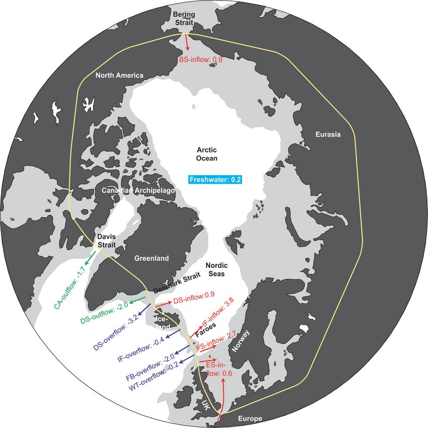
In most directions, the Arctic Mediterranean (AM) is sur- Figure 1. The Arctic Mediterranean (roughly represented by the
oceanic areas within the yellow curve) and its exchanges with
rounded by landmasses – Eurasia, North America, and
the rest of the World Ocean. Land areas are black. Ocean areas
Greenland – but a number of gaps connect the AM to the
shallower than 1000 m are light grey. Red arrows indicate inflow
rest of the World Ocean. The connection to the Pacific is branches. Dark blue arrows indicate overflow branches. Green ar-
the Bering Strait, while connections to the Atlantic1 are rows indicate surface outflow branches. Labels for arrows refer to
through the Canadian Arctic Archipelago and through the Sect. 2 with numbers indicating average volume transport in Sv
gaps between Greenland and the European continent (Fig. 1). (1 Sv = 106 m3 s−1 ) based on Table 1.
Through these gaps, flows pass into and out of the AM, trans-
porting water, heat, and salt. Here, our focus is only on the
transport of water (volume), not, for example, heat or fresh-
with the ambient waters from the Atlantic that they en-
water fluxes. The main aim of this manuscript is to synthesize
train en route, the overflow waters are understood to con-
the available observational evidence of the volume transports
tribute the main component of the North Atlantic Deep Wa-
of these flows and their variability into a consistent budget
ter (NADW; Gebbie and Huybers, 2010) which constitutes
and then to identify possible trends.
the deep branch of the AMOC (Dickson and Brown, 1994;
Though heat exchanges are the focus of regional climate
Hansen et al., 2004). Through ventilation and overflow, the
studies, AM exchanges also play an important role in the
AM is one of the main regions linking the atmosphere and
global climate through their influence on the Atlantic merid-
the deep World Ocean and the associated transport of atmo-
ional overturning circulation (AMOC). Between Greenland
spheric carbon dioxide into the deep ocean is critical for cli-
and the European continent, warm saline water flows from
mate change on long timescales (Sabine et al., 2004).
the Atlantic into the AM where it is cooled via air–sea ex-
The inflowing water from the Atlantic that does not re-
change processes. The waters are also freshened by runoff,
turn as overflow mixes with the Pacific inflow and leaves the
net precipitation, and mixing with Pacific waters (and ice
AM through the Canadian Arctic Archipelago and Denmark
melt), but still much of the resulting water mass is sufficiently
Strait as cold and relatively fresh “surface outflow” (Curry et
dense to be transported to greater depths through various pro-
al., 2014; de Steur et al., 2017).
cesses (e.g. Rudels et al., 1999).
Exchanges between the AM and the rest of the World
These dense water masses leave the AM through the deep
Ocean can therefore be grouped into three types of flow that
passages across the Greenland–Scotland Ridge and enter the
play important, but different, roles in the ocean and climate
Atlantic as overflow waters. They are much denser than the
systems: inflowof water from the Atlantic and Pacific into the
ambient water masses in the Atlantic and descend to deeper
AM, overflowof dense water at depth from the AM into the
levels to form bottom intensified boundary currents. Together
Atlantic, and surface outflowin the upper layers into the At-
1 Strictly speaking, all of the AM is part of the Atlantic Ocean, lantic (Fig. 2). In addition to these oceanic exchange flows,
but we will follow common practice and reserve the term “Atlantic” freshwater enters the AM as runoff, Greenland meltwater dis-
for those regions of the Atlantic Ocean that are outside the AM. charge, and through net precipitation (Aagaard and Carmack,
Ocean Sci., 15, 379–399, 2019 www.ocean-sci.net/15/379/2019/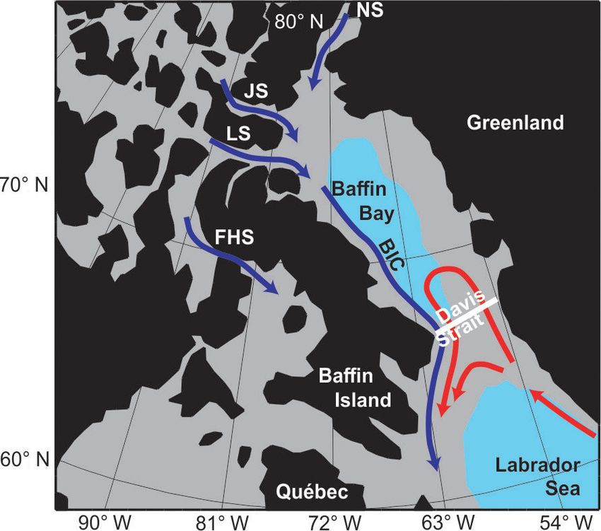
S. Østerhus et al.: Arctic Mediterranean exchanges                                                                                381

                                                                       2     The exchange branches and their observing systems

                                                                       In this section, we outline the main features of each indi-
                                                                       vidual exchange branch and of the observational systems
                                                                       used to quantify and monitor these exchanges. Following
                                                                       tradition (e.g. Hansen and Østerhus, 2000), we group them
                                                                       into the four (including freshwater) categories illustrated in
                                                                       Fig. 2. The distinction between overflows and surface out-
                                                                       flows is difficult, especially in the Denmark Strait where
                                                                       they flow together, and will be discussed later (Sects. 2.2.1
                                                                       and 2.3.2). Here, we use the following well-established crite-
Figure 2. In this study, the oceanic flows into and out of the AM      rion: σθ > 27.8 kg m−3 to define overflow (e.g. Dickson and
are grouped into three categories: inflows, overflows, and (surface)   Brown, 1994).
outflows. In addition, rivers, Greenland meltwater discharge, and         The observational evidence from the individual exchange
net ocean surface precipitation supply freshwater to the AM.           branches is highly variable. For some branches, we have time
                                                                       series of monthly averaged volume transport spanning more
                                                                       than two decades, although in some cases with gaps. For
1989; Serreze et al., 2006). Ice exports are not considered
                                                                       other branches, the time series are much shorter, or the ob-
here as the volume transports are low (same citations).
                                                                       servational evidence may be barely sufficient to provide one
   The important role of the AM in the World Ocean cir-
                                                                       number for the average transport without yielding any infor-
culation and global climate has been recognized for a long
                                                                       mation on temporal variations.
time. There have been many attempts to quantify the AM ex-
                                                                          To keep the text within readable limits, the descriptions
changes and establish a budget for the AM since the pioneer-
                                                                       provided in this section do not give complete information
ing attempt by Worthington (1970). Only recently, however,
                                                                       about each individual branch. Instead, our aim has been to
has the observational coverage become sufficiently compre-
                                                                       provide enough information to place each branch as a part
hensive and reliable that a consistent budget may be deter-
                                                                       of the whole exchange system and describe the observing
mined with confidence.
                                                                       methodology. For each branch, we list a few key references
   The flows into and out of the AM are an integral part of the
                                                                       for access to more detailed information. Where essential de-
AMOC, which is projected to weaken during the 21st century
                                                                       tails are not available in the literature, we have added infor-
(IPCC, 2013), and we discuss whether the observations show
                                                                       mation in the Supplement.
any indication of this.
   In terms of area and volume, the AM is dominated by
                                                                       2.1     Inflows
the Arctic Ocean, for which a budget was proposed by
Beszczynska-Möller et al. (2011). Much of the water mass
                                                                       Most of the water entering the AM comes from the At-
transformation and recirculation within the AM occurs, how-
                                                                       lantic Ocean (Atlantic inflow). The three main Atlantic in-
ever, in the Nordic Seas (Mauritzen, 1996). A budget for the
                                                                       flow branches pass through the deep passages across the
whole of the AM, which we try to establish here, will there-
                                                                       Greenland–Scotland Ridge (Fig. 3), which are discussed sep-
fore be different from a purely Arctic Ocean budget.
                                                                       arately. The remaining Atlantic inflows that we also have to
   In the following sections, we first list the main features and
                                                                       consider are the inflows over the Scottish shelf and through
observational systems for each individual exchange branch
                                                                       the English Channel. Here we combine these two flows into
and the data sets that we use. The combined results of these
                                                                       a “European Shelf Atlantic inflow”. Additionally, water from
data are given in Sect. 3 with the main focus on multi-year
                                                                       the Pacific Ocean (Pacific inflow) enters the AM through the
average transports, seasonal variations, and long-term trends.
                                                                       Bering Strait.
These results are discussed in Sect. 4, where we initially try
to assess whether the combined data set is consistent – e.g.
                                                                       2.1.1    Denmark Strait Atlantic inflow (“DS-inflow”)
do the combined average transports and their seasonal vari-
ations conserve mass. After that, we discuss what is perhaps
                                                                       The Denmark Strait, between Greenland and Iceland, is
the most important question of this study: are the total flows
                                                                       about 300 km wide with a sill depth of 630 m. Within the
into and out of the AM strengthening, weakening, or stable
                                                                       strait, Atlantic water flows towards the Iceland Sea mostly
over the time period covered by our observations? The paper
                                                                       over the Icelandic shelf. The Atlantic inflow passes north-
ends with Sect. 5 where we present our main conclusions and
                                                                       wards with the surface Irminger Current along the west coast
recommendations.
                                                                       of Iceland. When it reaches the Denmark Strait it splits into
                                                                       two branches with most of the water not flowing through
                                                                       the strait but flowing west across the Irminger Sea towards
                                                                       Greenland and subsequently southwestwards along the East

www.ocean-sci.net/15/379/2019/                                                                       Ocean Sci., 15, 379–399, 2019
382 S. Østerhus et al.: Arctic Mediterranean exchanges
vidual current-meter records probably due to fishing activity
in the area and occasional icebergs, but the transport record
is continuous since some of the moorings have always been
recovered.
The time series for DS-inflow volume transport used in
this study consists of monthly averages from October 1994
to December 2015.
2.1.2 Iceland–Faroe Atlantic inflow (“IF-inflow”)
Between Iceland and the Faroes, the Iceland–Faroe Ridge has
a sill depth around 480 m close to the Faroes, and is deeper
than 300 m over much of its extent. Across this ridge, there
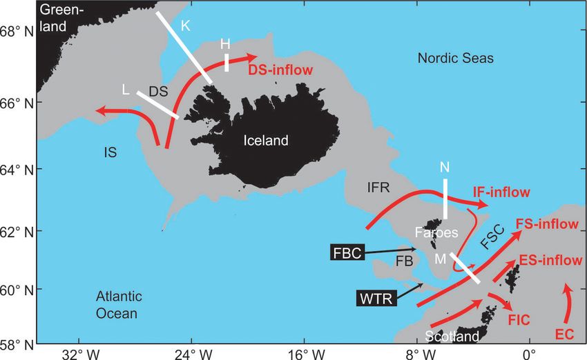
Figure 3. The Greenland–Scotland Ridge. Grey areas are shallower is an inflow of Atlantic water to the Nordic Seas in the upper
than 750 m. Red arrows show schematic flow patterns of the four layers (“IF-inflow”), whereas (southward flowing) overflow
Atlantic inflow branches. Thick white lines indicate monitoring sec- water crosses the ridge in the opposite direction at depth.
tions with labels referred to in the text (Sect. 2.1). Topographic Both exchanges occur over most of the length of the ridge,
features indicated are the Denmark Strait (DS), Irminger Sea (IS), but likely with large temporal and spatial variations (Tait,
Iceland–Faroe Ridge (IFR), Faroe Bank (FB), Faroe Bank Chan- 1967; Meincke, 1983; Perkins et al., 1998; Rossby et al.,
nel (FBC), Faroe–Shetland Channel (FSC), and Wyville Thomson
2009, 2018). Due to the high spatial and temporal variability
Ridge (WTR). “ES-inflow” includes contributions from the Fair Isle
Current (FIC) and the inflow through the English Channel (EC).
of these exchanges, a monitoring array located on the ridge
that could generate time series of IF-inflow volume transport
would need to be very extensive and would be vulnerable to
the intensive fishing activity. This has not been attempted.
Greenland continental slope. The other branch flows through Instead, monitoring has been established on a section (the
the Denmark Strait into the Iceland Sea and continues onto N section, Fig. 3) east of the ridge where the inflow cross-
the North Icelandic shelf where it flows eastwards along the ing the ridge is focused into a relatively narrow boundary
shelf as the North Icelandic Irminger Current (Stefánsson, current, the Faroe Current, which includes all the Atlantic
1962). water entering the AM in this region. This current flows east-
The method used for calculating the water mass compo- wards north of the Faroes, bounded on the north side by the
sition on the Hornbanki section (H section, Fig. 3) and the Iceland–Faroe Front (Tait, 1967; Hansen and Meincke, 1979;
transport of Atlantic water is described in detail by Jónsson Read and Pollard, 1992). The N section has been sampled 3–
and Valdimarsson (2005, 2016). We use CTD (conductivity– 4 times annually by CTD cruises since the late 1980s. Since
temperature–depth) profiles from the Látrabjarg and Kögur 1997, this has been complemented by an array of moored
standard sections that have typically been sampled 4 times ADCPs, deployed below the extent of fishing gear or in
annually for the period when moorings were present on the trawl-protected frames on the bottom. Based on the com-
Hornbanki section (L and K sections, respectively, Fig. 3). bined ADCP and CTD data, Hansen et al. (2003) derived
A station on the L section that always lies within the At- average estimates and time series of volume transport for the
lantic water flowing northwards and a station on the K sec- IF-inflow, representing the Atlantic water crossing the ridge.
tion that is within the Polar waters of the East Greenland The volume transport based solely on in situ observations
Current are combined with temperature measurements from was found to be well correlated with the sea level tilt on the
the Hornbanki mooring array (H section, Fig. 3) to calcu- section derived from altimetry data (Hansen et al., 2010),
late the water mass composition at the H section, assuming and a new algorithm was developed which combines data
that it is a mixture of Atlantic and Polar waters. The current- from altimetry and in situ observations (Hansen et al., 2015).
meter records from the H section are then used to calculate Based on this, the time series for IF-inflow volume transport
the transport of Atlantic water to the AM through the Den- used in this study consists of monthly averages from Jan-
mark Strait. The current-meter measurements started in 1994 uary 1993 to December 2015.
and have been maintained and made more extensive since
then (Jónsson and Valdimarsson, 2012). In 1999 the array 2.1.3 Faroe–Shetland Atlantic inflow (“FS-inflow”)
was extended from one mooring to three moorings and in
2012 a mooring was added north of the previous moorings. The gap in the Greenland–Scotland Ridge between the
From 1994 to 2009, velocity at the H section was measured Faroes and Scotland is called the Faroe–Shetland Channel
with single-point current meters, but starting in 2009 velocity (FSC). The deepest part of the channel is deeper than 1000 m.
measurements have been made mostly with acoustic Doppler Water of Atlantic origin usually fills the upper layers down to
current profilers (ADCPs). There are several gaps in the indi- 400–500 m across the whole channel, but a significant frac-
Ocean Sci., 15, 379–399, 2019 www.ocean-sci.net/15/379/2019/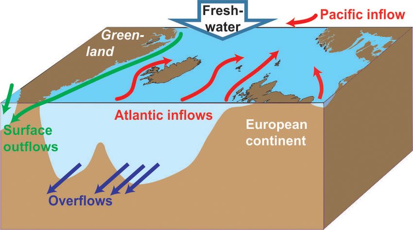
S. Østerhus et al.: Arctic Mediterranean exchanges                                                                            383

tion of that water originally crossed the ridge north of the      fortunately, this has not been systematically monitored and
Faroes, entered the Faroe Current, and bifurcated into the        observationally based estimates of its volume transport seem
FSC, where it flows southwestwards along the Faroe side           difficult to find.
of the channel (Fig. 3; Helland-Hansen and Nansen, 1909;             Despite this lack of observational evidence, the average
Meincke, 1978; Hátún, 2004; Berx et al., 2013). Most of this      volume transport over the Scottish shelf must at least be
water is believed to recirculate within the channel and join      equal to the average volume transport of the Fair Isle Cur-
the direct inflow continuing into the Norwegian Sea (Hansen       rent that passes into the North Sea through the gap between
et al., 2017).                                                    the Orkneys and Shetland – the Fair Isle Gap (Fig. 3). This
   Regular hydrographic surveys along standard sections           current was estimated by Turrell et al. (1990) to have an av-
crossing the channel have been carried out for more than          erage transport of 0.13 Sv. Their observations only covered
a century (Tait, 1957; Turrell, 1995) and, since the 1970s,       a few months, however, and Hill et al. (2008) have updated
these have been complemented with current-meter moorings          this value to 0.4 Sv, based on a combined observational and
and other instrumentation (Gould et al., 1985; Dooley and         modelling effort.
Meincke, 1981; Rossby and Flagg, 2012; Berx et al., 2013;            This value may thus represent a minimum average vol-
Rossby et al., 2018). In this study, we use data from the         ume transport over the Scottish shelf, but some of the wa-
only long-term transport monitoring effort (Østerhus et al.,      ter over the shelf may continue northeastwards to flow west
2001), consisting of CTD profiles and moored ADCP time            of Shetland rather than passing through the Fair Isle Gap.
series along a standard section (the Munken–Fair Isle sec-        Again, there is little observational evidence, but some in-
tion, labelled M in Fig. 3) starting in 1994. The recirculation   formation may be gained from measurements by a ferry-
of Atlantic water and intensive mesoscale activity (Sherwin       mounted ADCP (Rossby and Flagg, 2012). The focus of the
et al., 1999, 2006; Chafik, 2012) complicate the calculation      ADCP data acquisition was on larger scales; but from their
of volume transport. By combining the in situ observations        graphs and updated graphs reported by Childers et al. (2014),
with data from satellite altimetry, Berx et al. (2013) gener-     we estimate an additional ∼ 0.1 Sv of water flowing into the
ated a time series of volume transport of the FS-inflow with      AM, giving a total average volume transport of 0.5 Sv over
monthly estimates from January 1993 to September 2011,            the Scottish shelf inside of the M section.
here extended to December 2015.                                      The flows over the Scottish shelf and through the En-
   The time series generated by Berx et al. (2013) represents     glish Channel include less saline water from coastal areas
the Atlantic water flow between the shelf edges on both sides     upstream in addition to the more oceanic component. Thus,
of the channel. On the Faroe shelf, northwest of the shelf        the term “Atlantic” may be somewhat misleading but, for our
edge boundary of the channel, there is a flow between the         purpose, it is the total volume transport rather than the char-
islands and the shelf edge, which generally is directed south-    acteristics of the water that is important. These coastal water
westwards. Most of this is considered to belong to a quasi-       masses are therefore included in the ES-inflow.
closed shelf circulation around the Faroes (Larsen et al.,           From in situ observations, there is little evidence about
2008) and therefore is not advected into the AM. This shelf       the variations in volume transport, but satellite altimetry may
circulation is not included in the IF-inflow as it passes east-   be used for that purpose as long as we can assume geostro-
wards north of the Faroes (Hansen et al., 2003) and should        phy, which works well for the neighbouring FS-inflow (Berx
therefore not be included in the FSC either. For the conti-       et al., 2013). As elaborated on in the Supplement, we have
nental shelf region southeast of the FSC monitoring section,      therefore combined the established average transport value
there is, on the other hand, an Atlantic inflow, which is not     with sea level anomalies (SLA values) from altimetry to gen-
recirculated around the UK. That contribution is discussed in     erate monthly time series of ES-inflow with the additional as-
the next section, Sect. 2.1.4.                                    sumption of barotropic flow. This assumption probably leads
                                                                  to transport variations that are too high, but they are still low
2.1.4   European Shelf Atlantic inflow (“ES-inflow”)              in absolute terms and should not have much influence on the
                                                                  overall picture.
The European Shelf (ES)-inflow is the inflow of Atlantic wa-         In addition to the flow over the Scottish shelf, there is
ter between the southeastern boundary of the Faroe–Shetland       also an inflow of Atlantic water through the English Chan-
Channel monitoring system and the European continent.             nel, which according to the observations reported by Pran-
The previously discussed (Sect. 2.1.3) Atlantic water flow        dle (1993) has an average volume transport of ∼ 0.1 Sv. Al-
through the channel – the FS-inflow – has been monitored on       together, we will therefore use a value of (0.6 ± 0.2) Sv for
a section (the M section in Fig. 3) that terminates at a point    the average volume transport of the ES-inflow where the un-
just inside the shelf edge on the Scottish shelf with bottom      certainty value is estimated from the limited observational
depth of ∼ 150 m (Berx et al., 2013; bottom right extent of       evidence.
white line in Fig. 3). Between this point and the Orkneys,
there is a distance of ∼ 125 km (which we call here the Scot-
tish shelf), through which there may be appreciable flow. Un-

www.ocean-sci.net/15/379/2019/                                                                   Ocean Sci., 15, 379–399, 2019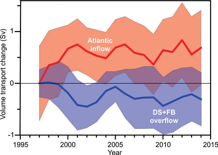
384                                                                           S. Østerhus et al.: Arctic Mediterranean exchanges

                                                                      dense water from the AM that are generally characterized as
                                                                      “overflow”. In the literature, various criteria have been used
                                                                      to define overflow – either in terms of temperature or den-
                                                                      sity. In this study, we use the most common definition that
                                                                      σθ > 27.8 kg m−3 (e.g. Dickson and Brown, 1994). We also
                                                                      follow common practice (e.g. Hansen and Østerhus, 2000) to
                                                                      group the overflow into four different branches (Fig. 5).

                                                                      2.2.1    Denmark Strait overflow (“DS-overflow”)

                                                                      About half of the dense overflow waters from the Nordic Seas
                                                                      enter the North Atlantic through Denmark Strait, where the
                                                                      DS-overflow becomes one of the major sources of NADW
                                                                      (e.g. Dickson and Brown, 1994). The overflow plume cross-
                                                                      ing the passage between Iceland and Greenland is generally
Figure 4. The Bering Strait has two channels separated by the
Diomede Islands (DI). Red arrows indicate annual mean flow paths.
                                                                      found at a depth below 250 m, although close to the Icelandic
White circles mark mooring positions (A1, A2, A3, A4). Dashed ar-     shelf warm and saline Atlantic water frequently occupies the
row marks the Alaskan Coastal Current (ACC), present seasonally.      passage down to the bottom (Mastropole et al., 2017).
Grey areas are shallower than 100 m.                                     The width of the Denmark Strait, which is deeper than
                                                                      350 m, covers a distance of 60 km only. Here, the over-
                                                                      flow plume is most intense with downstream velocities ex-
2.1.5    Bering Strait Pacific inflow (“BS-inflow”)                   ceeding 1 m s−1 and near-bottom temperatures below 0 ◦ C.
                                                                      Mesoscale eddy activity is well documented, and occurs with
The Bering Strait is a narrow (width ∼ 85 km) and shallow             periods of 2–10 days (Ross, 1984; Käse et al., 2003; Fischer
(sill depth ∼ 50 m) strait connecting the Pacific and Arctic          et al., 2015), whereas seasonal variability is small and no sig-
oceans (Fig. 4). Since 1990, year-round measurements have             nificant long-term trends have been found so far (Jochumsen
been maintained in the strait almost without interruption, typ-       et al., 2012). Moored instrumentation for current profile mea-
ically at 2–3 sites (Fig. 4) located within one or both of the        surements (ADCPs) have been installed in this part of the
two channels of the strait (sites A1 and A2), and typically           passage (the L section in Fig. 5). The standard deployment
also at a mid-strait site, A3, slightly to the north, at a location   consists of two moorings: one at 650 m depth at the deepest
found to give a useful average of the flows from the two chan-        part of the sill of the strait, the other 10 km further towards
nels (e.g. see Woodgate et al., 2015, for discussion). In 2001,       Greenland at 570 m depth. These positions cover the over-
a mooring (A4) was added in the eastern side of the eastern           flow current core, but a large volume of dense water on the
channel to monitor the warm low-salinity Alaskan Coastal              Greenland shelf is not accounted for.
Current (ACC) present seasonally (Woodgate et al., 2015).                Velocities on the shelf are small, but the distance to the
   In the 1990s, velocities at the mooring sites were measured        coast of Greenland is still more than 250 km, where some
mostly by single-point current meters; but since 2007, veloc-         dense water is transported southward (de Steur et al., 2017).
ity measurements have been made predominantly with AD-                In earlier publications, this transport was inferred from a
CPs. Based on the observed dominantly barotropic and spa-             model and added to the transport calculations obtained by the
tially homogeneous nature of the flow (away from the ACC),            moorings (Macrander et al., 2005; Jochumsen et al., 2012).
volume transport is calculated by multiplication of velocity          In 2014/2015, however, an experiment was made with five
and cross-sectional area for the strait (Woodgate, 2018).             moorings on the L section, from which a new algorithm was
   Over the period of monitoring (1990 to present), there has         developed to derive volume transport from the historical AD-
been a statistically significant increase in annually averaged        CPs observations (Jochumsen et al., 2017). The monthly av-
volume transport from 0.8 Sv in the beginning of the pe-              eraged DS-overflow transport values used here are based on
riod (Roach et al., 1995) to ∼ 1.2 Sv by the end (Woodgate,           this algorithm and extend from May 1996 to December 2015,
2018). Here, we use the monthly mean volume transports                although with gaps.
from August 1997 to December 2013.                                       A quality check on this new time series is provided by the
                                                                      experiment reported by Harden et al. (2016) with a dense
2.2     Overflows                                                     mooring array on the K section (Fig. 5) lasting from Septem-
                                                                      ber 2011 to July 2012. For the overlapping period (336 days),
The only deep connections between the AM and the rest of              our data set based on Jochumsen et al. (2017) has an average
the World Ocean are the gaps in the Greenland–Scotland                transport of 3.1 Sv, whereas Harden et al. (2016) find 3.5 Sv.
Ridge and only through these gaps do we find the flows of             Considering the uncertainties reported (±0.5) and possible

Ocean Sci., 15, 379–399, 2019                                                                     www.ocean-sci.net/15/379/2019/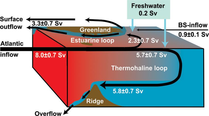
S. Østerhus et al.: Arctic Mediterranean exchanges                                                                                   385

                                                                         al., 2016). Measurements within the Western Valley have
                                                                         not, however, shown any clear evidence of strong overflow
                                                                         (Perkins et al., 1998; Beaird et al., 2013); and based on a
                                                                         dedicated field experiment from August 2016 to May 2017,
                                                                         Hansen et al. (2018) argue that the long-term average over-
                                                                         flow transport through the Western Valley is less than 0.1 Sv.
                                                                            Following these recent results, we use 0.4 Sv for the aver-
                                                                         age transport of IF-overflow with an uncertainty of ±0.3 Sv.
                                                                         This quantity for the average transport may seem small when
                                                                         the bottom current downstream of the Western Valley is taken
                                                                         into account (Perkins et al., 1998; Olsen et al., 2016), but the
                                                                         volume transport of this current is not well constrained by ob-
                                                                         servations and neither are its origin and en-route entrainment
Figure 5. Overflow and surface outflow branches across the               of Atlantic water. From bottom temperature measurements
Greenland–Scotland Ridge. Grey area is shallower than 750 m. Ar-         (Olsen et al., 2016), it also seems unlikely that much of this
rows indicate schematic flow patterns of the four overflow branches      water would fulfil the criterion for overflow. Seasonal and
(dark blue, discussed in Sect. 2.2) and the one surface outflow across   long-term variations in the IF-overflow cannot be addressed
the ridge (green, discussed in Sect. 2.3). Thick white lines indicate    with the observational material available.
monitoring sections with labels referred to in the text. Topographic
features indicated are Iceland–Faroe Ridge (IFR), Faroe–Shetland
Channel (FSC), and Western Valley (WV).
                                                                         2.2.3   Faroe Bank Channel overflow (“FB-overflow”)

                                                                         The Faroe Bank Channel is the deepest passage across the
water mass transformations between the two sections, this                Greenland–Scotland Ridge with a sill depth of 840 m. The
comparison is encouraging (Jochumsen et al., 2017).                      bottom layer in this channel is continually dominated by cold
                                                                         overflow water that flows over the sill with core speed usu-
2.2.2   Iceland–Faroe Ridge overflow (“IF-overflow”)                     ally exceeding 1 m s−1 out into the Atlantic (Hermann, 1959;
                                                                         Borenäs and Lundberg, 1988; Saunders, 2001; Hansen and
Overflow across the Iceland–Faroe Ridge was identified                   Østerhus, 2007; Hansen et al., 2016).
more than a century ago (Knudsen, 1898) and it has long                     Since the early estimates by Hermann (1967) and
been known that it may occur at many locations along the                 Sætre (1967), several transport estimates for the FB-overflow
ridge (Hermann, 1967; Meincke, 1983). From the results                   have been published. Here, we use the most comprehensive
of the “Overflow 0 60” expedition, Hermann (1967) esti-                  data set consisting of data from long-term ADCP moorings
mated a total volume transport of 1.1 Sv for the IF-overflow.            on the V section (Fig. 5), combined with other moored instru-
Based on moorings and hydrographic observations, Perkins                 mentation and regular CTD cruises (Hansen et al., 2016). The
et al. (1998) estimated at least 0.7 Sv overflow close to Ice-           primary time series generated from these observations is the
land, and Beaird et al. (2013) used measurements from au-                “kinematic overflow”, which is based on velocity (ADCP)
tonomous Seagliders to find a minimum of 0.8 Sv for the to-              measurements alone. This time series has an average volume
tal overflow across the ridge. However, observationally based            transport of 2.1 Sv, which, however, includes 0.2 Sv of water
information on temporal variations or time series of total IF-           less dense than the established criterion (σθ ≥ 27.8 kg m−3 ).
overflow have not been published.                                        For our purpose, the time series has therefore been converted
   The Iceland–Faroe Ridge may conveniently be divided                   by multiplying the values with a fixed ratio of (2.1–0.2)/2.1.
into two parts at the latitude of 63◦ N (Fig. 5). Across the             The series contains monthly averaged volume transport from
southern (Faroese) part, the overflow is considered to be in-            December 1995 to December 2015, although with gaps dur-
termittent (Østerhus et al., 2008) and from their extensive              ing the annual servicing periods.
Seaglider experiment, Beaird et al. (2013) estimated an av-
erage volume transport of that part of the overflow of 0.3 Sv            2.2.4   Wyville Thomson Ridge overflow
with an uncertainty almost as high.                                              (“WT-overflow”)
   Across the northern (Icelandic) part, the overflow has gen-
erally been thought to be more persistent (Østerhus et al.,              The Wyville Thomson Ridge has a sill depth of around 600 m
2008), especially the overflow through the northernmost pas-             with intermittent overflow of dense water both at the deepest
sage across the ridge, labelled the Western Valley (Fig. 5).             point at the centre of the ridge and at the far west of the ridge
This is partly from theoretical arguments and partly from ob-            (Ellett and Roberts, 1973; Sherwin et al., 2008; Johnson et
servations of a strong and persistent bottom current down-               al., 2017). This flow, the WT-overflow, is channelled by to-
stream from the Western Valley that seems to have been                   pography into the Ellett Gully before entering the Rockall
generated by IF-overflow (Perkins et al., 1998; Olsen et                 Trough to the south. The flow through the Ellett Gully has

www.ocean-sci.net/15/379/2019/                                                                          Ocean Sci., 15, 379–399, 2019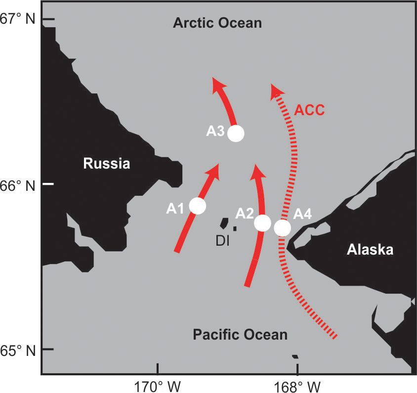
386                                                                       S. Østerhus et al.: Arctic Mediterranean exchanges

primarily been monitored by ADCP moorings but also by a
CTD section (the W section in Fig. 5).
   The time-varying nature of WT-overflow necessitates the
combination of volume transports with proportions of Faroe–
Shetland Channel Bottom Water (FSCBW) in order to pro-
duce a transport comparable to other overflow time series
(Sherwin et al., 2008). In this method, the volume transport
through the Ellett Gulley, as measured by the moored ADCP,
is weighted by the proportion of FSCBW in the water col-
umn, calculated from linear mixing between FSCBW (de-
fined as having a temperature of 0 ◦ C) and Atlantic Water
(defined as having a temperature of 8.5 ◦ C). The method as-
sumes temperature decreases linearly from the depth of the
8.5 ◦ C isotherm to the seabed, and that the isotherms are hor-
izontal. Sensitivity tests suggest that the error associated with
                                                                    Figure 6. Outflow from the Arctic Ocean through the Canadian
these assumptions is less than ±20 % (±0.04 Sv). The time
                                                                    Arctic Archipelago. Flows through Nares Strait (NS), Jones Sound
series of WT-overflow used in this study is based on this
                                                                    (JS), Lancaster Sound (LS), and Fury and Hecla Strait (FHS) as well
method and consists of monthly averages from May 2006               as the Baffin Island Current (BIC) are indicated by blue arrows. The
to May 2013, although there is a data gap from June 2009 to         thick white line indicates the Davis Strait monitoring section. Red
May 2011 due to instrument loss.                                    arrows indicate water flowing northwards through the section before
   The definition of FSCBW is slightly denser than our cri-         recirculating, joining, and partly mixing with the Arctic Ocean out-
terion for overflow water (27.8 kg m−3 ) and thus 0.2 Sv is         flow and exiting south again. Grey areas on the map are shallower
a lower bound for the volume transport. Previous measure-           than 1000 m.
ments in the region have suggested transports between 0.1
and 0.3 Sv (Hansen and Østerhus, 2000). We therefore use
the time series of WT-overflow transport based on the method        the eastern side of the strait, consists of the low-salinity West
of Sherwin et al. (2008) but attach an uncertainty of ±0.1 Sv.      Greenland Current (WGC) on the shelf and the warm, salty
                                                                    West Greenland Slope Current (WGSC) of North Atlantic
                                                                    origin over the slope (Curry et al., 2014). The WGC is a com-
2.3     Surface outflows
                                                                    bination of the East Greenland Current (EGC) flowing south-
In addition to the overflow of dense water through the deep         ward from the Arctic through Fram Strait (de Steur et al.,
passages across the Greenland–Scotland Ridge, the AM also           2009) and the East Greenland Coastal Current (EGCC) aris-
exports water that is less dense and remains in the upper lay-      ing from the addition of East Greenland coastal inflow and
ers. The flow of these water masses is denoted as “surface          glacial runoff (Bacon et al., 2002; Sutherland and Pickart,
outflow” or just “outflow” and it may be seen as two separate       2008). The WGSC is a branch of the North Atlantic Cur-
branches passing on either side of Greenland.                       rent that enters and circulates cyclonically in the Irminger
                                                                    Sea and continues along the East Greenland slope seaward
                                                                    of the EGC around Greenland (Cuny et al., 2002; Myers et
2.3.1    Canadian Arctic Archipelago surface outflow
                                                                    al., 2007). Both the WGC and WGSC flow around the south-
         (“CA-outflow”)
                                                                    ern tip of Greenland and then turn north toward Baffin Bay.
The Canadian Arctic Archipelago (CAA) is a collection of            Transport through Davis Strait has been monitored using a
numerous islands separated by narrow sounds. Through these          mooring array north of the sill that includes velocity, tem-
sounds and through the Nares Strait, separating the CAA             perature, and salinity measurements from 15 moorings span-
from Greenland, there is a net flow of water from the Arc-          ning the full width (330 km) of the strait accompanied by
tic Ocean towards the Labrador Sea (Fig. 6). Measurements           autonomous Seaglider surveys (Curry et al., 2014).
of these flows are difficult due to ice, strong tidal currents,        Transport through Davis Strait is used to represent the CA-
recirculation, and proximity to the magnetic pole. Neverthe-        outflow in this study. We use monthly averaged volume trans-
less, volume transport has been estimated from observations         ports from October 2004 to September 2010. There is a small
at several locations (Melling et al., 2008).                        component of the Arctic Ocean outflow that bypasses Baffin
   Davis Strait connects Baffin Bay to the Labrador Sea and         Bay and flows through Fury and Hecla Strait (Fig. 6). Its vol-
has a sill (640 m depth) that limits deep exchanges between         ume transport is not well constrained but has been estimated
the two. Exchanges through the strait are predominantly two         to be less than 0.1 Sv (Straneo and Saucier, 2008). It will not
way and topographically steered (Tang et al., 2004). South-         be included here.
ward flow, on the western side of Davis Strait, carries inputs
from the integrated CAA through flows. Northward flow, on

Ocean Sci., 15, 379–399, 2019                                                                     www.ocean-sci.net/15/379/2019/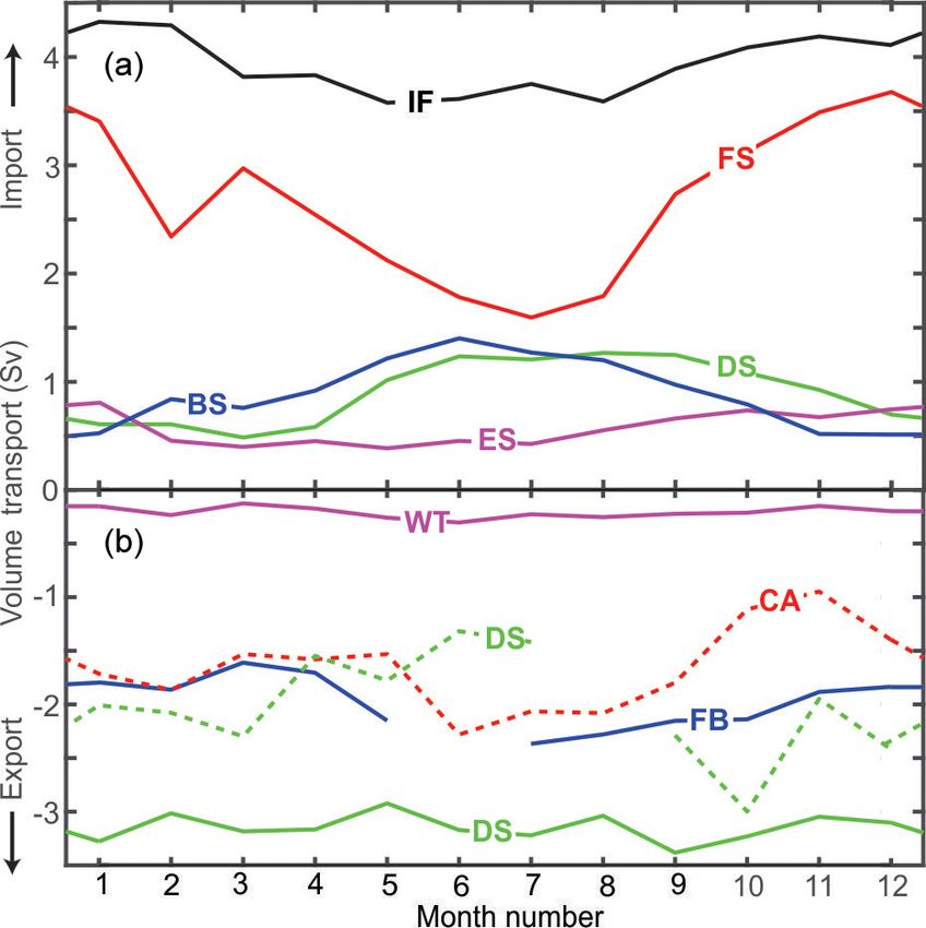
S. Østerhus et al.: Arctic Mediterranean exchanges                                                                              387

2.3.2    Denmark Strait surface outflow (“DS-outflow”)              nitudes, they are commonly reported in millisverdrup (mSv
                                                                    where 1 mSv = 10−3 Sv).
The surface outflow through the Denmark Strait is difficult            The freshwater budget of the Arctic Ocean was pioneered
to monitor. At times it may flow through a large part of the        by Aagaard and Carmack (1989) and updated by Serreze et
width of the strait, requiring a wide and dense mooring ar-         al. (2006) who reported a net precipitation of 65 mSv and a
ray while the component flowing over the East Greenland             runoff of 102 mSv to the Arctic Ocean. Including also the
shelf is inundated with icebergs that are very destructive to       Nordic Seas, Dickson et al. (2007) added 20 mSv of net pre-
moored instrumentation. It therefore comes as no surprise           cipitation and 34 mSv of runoff from the Baltic, the Norwe-
that observation-based transport values of the DS-outflow           gian coast, and Greenland. Another 9 mSv enter the Canadian
have been late to arrive.                                           Arctic Archipelago from Greenland according to Dickson et
   The values used here are mainly based on the experiment          al. (2007). This yields a total freshwater input to the tradi-
described in Sect. 2.2.1 with a dense mooring array along the       tional AM of 230 mSv, which we round to 0.2 Sv with an
K section (Fig. 5) from September 2011 to July 2012 (Harden         estimated uncertainty less than 0.1 Sv. Since we also include
et al., 2016). There, the focus was on the dense-water com-         the North Sea in our definition of the AM (Fig. 1), there are
ponent (σθ > 27.8 kg m−3 ), but the transport of the less dense     additional inputs, especially river runoff from Belgium, the
water masses (σθ < 27.8 kg m−3 ) could also be derived from         Netherlands, and Germany into the North Sea, but they are
the observations as reported by de Steur et al. (2017). They        only a few millisverdrup and too small to affect this value
estimated the average transport of this upper-ocean compo-          (Radach and Pätsch, 2007).
nent to be 1.8 Sv towards the southwest with an uncertainty            Most of the freshwater contributions exhibit strong season-
of the order of ±0.5 Sv. This value does not, however, cover        ality. According to Serreze et al. (2006), the net precipitation
the East Greenland shelf region adequately.                         to the Arctic Ocean is more than twice as high in July as in
   To amend this, we add data from additional inshore moor-         March and river runoff to the Arctic Ocean has an even more
ings on the K section from 2012 to 2014 reported by de Steur        pronounced seasonal variation. A similar, although less ex-
et al. (2017). From these additional data, monthly averages         treme, seasonal variation has been reported for river runoff
of the transport over the shelf can be generated, and we add        to the Baltic (Bergström and Carlsson, 1994). Within the un-
these to the monthly averages from the 2011–2012 experi-            certainties generally applying to this study, it therefore seems
ment (Fig. 9b in de Steur et al., 2017). In this way, we obtain a   safe to assume a seasonal variation of Freshwater input to
time series of 11 months from September 2011 to July 2012,          the AM with amplitude around 0.1 Sv and maximum around
which should include the total surface outflow through the          July.
Denmark Strait. The validity of this approach is of course             In addition to seasonal, there are also long-term variations
dependent on the stationarity of the seasonal cycle over the        and Haine et al. (2015) suggest that net precipitation and
shelf, which is questionable, but the modification due to the       runoff to the Arctic Ocean and Canadian Arctic Archipelago
addition of the 2012–2014 inshore moorings is small.                were greater in the 2000s than for 1980–2000. The observa-
   On this basis, we have estimated a value of 2.0 Sv for the       tional evidence for this is, however, weak and in any case
average DS-outflow. This value is composed of two non-              within the quoted uncertainty. Thus, it will be ignored here.
concurrent contributions, the dominant of which was based
on only 11 months of observations. It must therefore be
treated with caution, as must the seasonal variation indicated
by the data, which shows a pronounced winter-intensification        3   Results
of the DS-outflow. A strong seasonality of the flow over the
Greenland slope is, however, supported by more prolonged            As described in the previous section, monthly transport val-
current measurements in this region (Jónsson, 1999). The            ues are available for almost all of the oceanic exchange
transport of the East Greenland Current at 74◦ N was also           branches into or out of the AM, although of highly variable
found to be subject to a large seasonal cycle related to the        duration and completeness. These monthly averaged values
wind-driven gyre in the Greenland Sea (Woodgate et al.,             (ignoring the fact that months have different number of days)
1999).                                                              are the basic data set used in this study (Table 1). The one
                                                                    exception is the IF-overflow that has not been systematically
                                                                    monitored and for which we only have estimated a typical
2.4     Runoff and precipitation (“Freshwater input”)               or “average” transport value and its uncertainty. Likewise,
                                                                    for the Freshwater input we only have an average value and
In addition to oceanic inflows, water enters the AM by net          a seasonal amplitude. In the following, we present the av-
precipitation (precipitation minus evaporation) and runoff          erage transports, as determined from the various data sets
from rivers as well as land-ice melting into the sea, which         (over differing time-periods), as well as their variations on
we consider collectively as “Freshwater input”. Since the           seasonal and long-term timescales. Transport values are de-
various freshwater contributions have relatively small mag-         fined as positive into the AM and negative out of the AM.

www.ocean-sci.net/15/379/2019/                                                                    Ocean Sci., 15, 379–399, 2019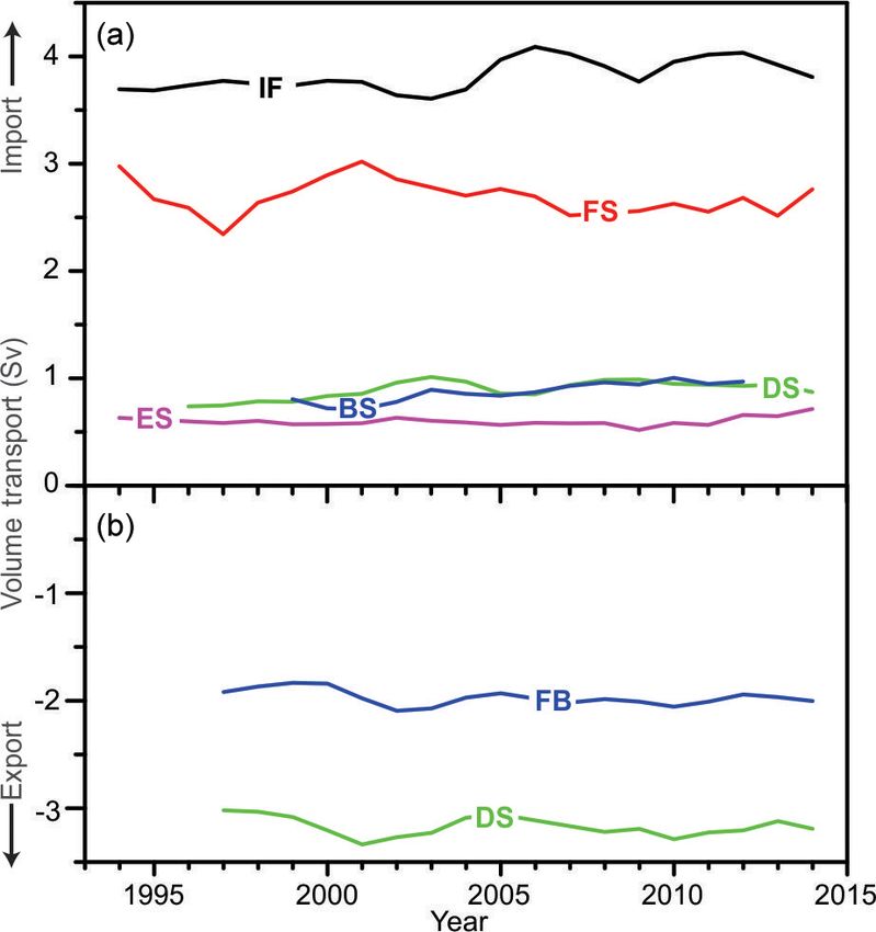
388                                                                             S. Østerhus et al.: Arctic Mediterranean exchanges

Table 1. Observational characteristics of each AM-exchange branch. The full period of observations is listed with the number of months
observed (Months) and the number of missing months (Gaps). The uncertainties of the average values are based on the information in
Sect. 2. The average transport values (Avg.) are positive into the AM and negative out of the AM. SD is the standard deviation of the monthly
averages. References to the sources for the data are listed for each branch in Sect. 2. For IF-overflow and Freshwater, time series are not
available (NA).

       Branch full name             Branch abbreviation     Period yyyy/mm–yyyy/mm         Months     Gaps      Avg. (Sv)    SD (Sv)
       Inflows:
       Denmark Strait Atlantic      DS-inflow               1994/10–2015/12                    250        5     0.9 ± 0.1         0.3
       Iceland–Faroe Atlantic       IF-inflow               1993/01–2015/12                    276        0     3.8 ± 0.5         0.6
       Faroe–Shetland Atlantic      FS-inflow               1993/01–2015/12                    276        0     2.7 ± 0.5         1.1
       European Shelf Atlantic      ES-inflow               1993/01–2015/12                    276        0     0.6 ± 0.2         0.3
       Bering Strait Pacific        BS-inflow               1997/08–2013/12                    197        0     0.9 ± 0.1         0.4
       Overflows:
       Denmark Strait               DS-overflow             1996/05–2015/12                    218       18   −3.2 ± 0.5          0.4
       Iceland Faroe Ridge          IF-overflow             NA                                                −0.4 ± 0.3
       Faroe Bank Channel           FB-overflow             1995/12–2015/12                    206       35   −2.0 ± 0.3          0.3
       Wyville Thomson Ridge        WT-overflow             2006/05–2013/05                     61       24   −0.2 ± 0.1          0.1
       Surface outflows:
       Canadian A. Archipelago      CA-outflow              2004/10–2010/09                     72        0   −1.7 ± 0.2          0.7
       Denmark Strait               DS-outflow              2011/09–2012/07                     11        0   −2.0 ± 0.5          0.5
       Runoff and precipitation:
       Freshwater input             Freshwater              NA                                                        0.2

3.1   Average volume transports                                          almost twice that of the IF-inflow even though the IF-inflow
                                                                         has a higher average transport.
Combining all the inflow transports with the freshwater in-                 Some of this variability seems to derive from systematic
put, we get the total “AM-import”, which has an average                  seasonal variations as indicated in Fig. 7, where we have
value of 9.1 Sv. Likewise, we can combine all the overflow               compared seasonal variations during the most complete 6-
transports with the surface outflow transports to an “AM-                year period. The inflow branches seem to have different sea-
export” with an average value of −9.5 Sv. Hence, the export              sonal variations (Fig. 7a), with the IF-inflow, the FS-inflow,
exceeds the import so that the average Net import (AM im-                and the ES-inflow being strongest around the turn of the
port + AM export) is −0.4 Sv. Combining the various uncer-               year, whereas the BS-inflow and the DS-inflow are strongest
tainty terms, this number has an uncertainty exceeding 1 Sv.             in summer. For the overflow and surface outflow branches,
   Thus, the imbalance in the average Net import is within               the picture seems less clear (Fig. 7b) and most of the export
the combined uncertainties even though the various numbers               branches do not exhibit any clear seasonality.
in Table 1 are averaged over widely different periods. The                  To get a more complete impression of the seasonal varia-
most complete coverage is during a 6-year period, from Oc-               tion, the monthly transport values for the five inflow branches
tober 2004 to September 2010, in which there are 53 months               in Fig. 7a have been summed to give the total AM import
with data from all of the inflow branches, from the DS-                  when the Freshwater input is neglected. Subtracting the over-
overflow, the FB-overflow, and from the CA-outflow. The                  all average, we get the seasonal import anomaly, which is
sum of the transport values for all of these branches in these           shown as the red curve in Fig. 8. Similarly, the blue curve
months are all inside the error estimate for the sum based on            in that figure shows the seasonal anomaly of the AM export;
the full periods (Table 1).                                              although note that this neglects the IF-overflow and missing
                                                                         months for the FB-overflow and DS-outflow that had to be
3.2   Seasonal variation                                                 interpolated to get a complete seasonal coverage.
                                                                            Combining the red and blue curves in Fig. 8, we get the
Table 1 also lists the standard deviation of the monthly trans-
                                                                         seasonal anomaly of the Net import for those branches that
port values for each individual branch and some branches are
                                                                         have been sufficiently well observed (black curve). It seems
clearly more variable than others, especially when consider-
                                                                         to indicate a maximum in November and minimum in Au-
ing the ratio between standard deviation and average trans-
                                                                         gust with an amplitude of the order of 1 Sv. A more detailed
port. Thus, the monthly standard deviation of the FS-inflow is

Ocean Sci., 15, 379–399, 2019                                                                          www.ocean-sci.net/15/379/2019/
S. Østerhus et al.: Arctic Mediterranean exchanges 389
Table 2. Linear trends of annual averages of the five inflow branches
individually and summed and of the DS-overflow. Only years with
complete coverage (no months missing) are included and the num-
ber of years is listed. The trend is represented by its value ± its
95 % confidence interval. Branches with trends that are significant
at the 95 % level are marked in bold. The last column lists relative
trends (Rel. tr.) determined by dividing the trends with the average
transports from Table 1.
Branch Period Years Trend Rel. tr.
(Sv yr−1 ) (yr−1 )
DS-inflow 1997–2015 18 0.004 ± 0.011 0.4 %
IF-inflow 1993–2015 23 0.012 ± 0.013 0.3 %
FS-inflow 1993–2015 23 −0.006 ± 0.024 −0.2 %
ES-inflow 1993–2015 23 0.003 ± 0.005 0.5 %
BS-inflow 1998–2013 16 0.016 ± 0.014 1.8 %
All inflows 1998–2013 15 0.040 ± 0.046 0.4 %
DS-overflow 1997–2015 14 −0.007 ± 0.015 −0.2 %
Figure 7. Seasonal variation in five inflow branches (a), three over-
flow branches (continuous lines in b), and two surface outflow
branches (dashed lines in b). All the lines are based on observations
taken between October 2004 and September 2010 except for the
DS-outflow (dashed green line in b), which is based on the Septem-
ber 2011 to July 2012 period with inshore values from 2013 to 2014
(Sect. 2.3.2). We have no seasonal information for the IF-overflow
and so it is not included in this plot. See Table 1 for abbreviations.
discussion of this imbalance will be presented in Sect. 4.2,
but it is worth emphasizing that this curve is not based on
Figure 8. Seasonal anomalies of the combined inflow branches
a very homogeneous data set. The inflow branches and the
(red) and the combined overflow and surface outflow branches
CA-outflow had no gaps in the selected period, but that was
(blue) for the same periods as in Fig. 8, where missing months
not the case for the overflow branches and our data for the have been interpolated. The black curve is the sum of the other two
DS-outflow only cover 11 months and they are outside the curves and represents the anomaly of the Net import when the IF-
selected period. overflow (order 0.4 Sv in the annual mean) and Freshwater input
(order 0.2 Sv in the annual mean) are neglected.
3.3 Long-term variations
Only the five inflow branches and the two main overflow acterized by stability rather than change – at least over the
branches have been observed over sufficiently long periods to observed period.
allow a meaningful investigation of possible long-term vari- A more illustrative picture of the long-term variation is
ations or trends. The FB-overflow has months missing for presented in Fig. 9, which shows low-pass filtered series gen-
almost every year but for the other branches, annual averages erated by averaging all observed months (up to 36) in 3-year
may be computed for most of the years within the observing periods. For some branches, months were missing for some
period. Based on these annual averages, Table 2 lists linear of the 3-year periods, but never more than 6 months. Thus,
trends as calculated by linear regression of annual volume all the points in Fig. 9 are averaged over at least 30 months.
transport over time. The curves in Fig. 9 are consistent with Table 2 with only
Except for the BS-inflow, the trends in Table 2 are less weak trends for most of the branches and relatively small
than their confidence intervals, which are calculated with- variations.
out taking serial correlation (autocorrelation) into account. The longest time series considered here are for the four At-
The number of degrees of freedom are therefore probably lantic inflow branches and the two main overflow branches.
too high and thus these confidence intervals are likely to be From 1996 to 2015, the Atlantic inflow branches had almost
underestimates of the real uncertainty in the trend. The ex- complete coverage and the total volume transport of these
changes between the AM and the Atlantic are therefore char- branches had at most 2 months missing in every 3-year pe-
www.ocean-sci.net/15/379/2019/ Ocean Sci., 15, 379–399, 2019390 S. Østerhus et al.: Arctic Mediterranean exchanges
Figure 10. Low-pass filtered (3-year running mean) volume trans-
port change (from the value in 1997) of the sum of the four At-
lantic inflow branches (thick red line) and the sum of the two main
overflow branches (thick blue line). The value for each year is the
average of the de-seasoned values for all observed months of the
year, the preceding year, and the following year. The coloured areas
Figure 9. Low-pass filtered (3-year running mean) volume trans-
represent the 95 % confidence interval (Sect. S2).
port of the five inflow branches (a) and the two main overflow
branches (b). The value for each year is the average of the values for
all observed months of the year, the preceding year, and the follow-
ing year. To minimize bias from missing months, the values have ask whether it is within acceptable bounds. The following
been de-seasoned before averaging (Sect. S2 in the Supplement). Sects. 4.1 and 4.2 therefore address what constraints nature
puts on the average value and seasonal variation in the net
import. Another problem is that the individual observational
riod. Thus the thick red line in Fig. 10 should give a good systems do not combine into a contiguous whole. This is
representation of the variations of the total Atlantic inflow discussed in Sect. 4.3. The implications of the apparent im-
during these 18 years. The sum of the two main overflow balances in our results for data quality are summarized in
branches has less complete coverage, but the de-seasoned 3- Sect. 4.4. In a very simplified picture, the AM may be seen
year running mean (thick blue line in Fig. 10) still should as a double estuary with an estuarine as well as a thermoha-
give an indication of the variation in this series. line loop. In Sect. 4.5, we estimate the relative strengths of
Figure 10 shows the change in inflow/overflow relative to these two loops and their sources. After that, in Sect. 4.6, we
their late 1990s values. For both the total Atlantic inflow and address the important question: have the total flows into and
the sum of the two main overflow branches, Fig. 10 seems out of the AM been weakening, strengthening, or remained
to indicate strengthening from the late 1990s to 2002 with stable within our observational period?
little overall change after that. When taking the uncertainties
(coloured areas in Fig. 10) into account, the statistical signif- 4.1 Constraints on the average AM-exchange budget
icance of the apparent changes seems low, however, and the
overall message is one of stability. The ultimate criterion for a consistent exchange budget is
mass conservation. When there is an imbalance between im-
port and export, the total mass within the AM must change
4 Discussion accordingly. If there were no density changes, the mass bal-
ance would be equivalent to volume balance (continuity). An
The results presented in the previous section are from a wide imbalance of 0.1 Sv that is sustained for a year would then
and inhomogeneous set of observational systems. The first imply a sea level change around 20 cm on average over the
question to ask is therefore whether they are mutually consis- whole AM. This is considerably more than available obser-
tent. From Table 1, the estimated AM export is 0.4 Sv higher vations indicate for inter-annual sea level variations (Volkov
than the AM import, but this imbalance is well within the and Pujol, 2012; Andersen and Piccioni, 2016), although ob-
uncertainties quoted in the table and needs no further expla- servational evidence is missing for much of the Arctic Ocean.
nation. Whether to expect a zero imbalance in our data set is, Basin-wide GRACE Ocean Bottom Pressure data suggest in-
however, not as obvious as might be thought and is discussed terannual trends between 2002 and 2006 of only a few cen-
in Sect. 4.1. timetres (< 5 cm yr−1 ) over the Arctic basin, and of varying
Similarly, the Net import in our data set appears to sign (Morison et al., 2007); this is further evidence that an
have a non-zero seasonal variation (Fig. 8) and we need to imbalance of 0.1 Sv is unrealistic.
Ocean Sci., 15, 379–399, 2019 www.ocean-sci.net/15/379/2019/You can also read