Glacier Image Velocimetry: an open-source toolbox for easy and rapid calculation of high-resolution glacier velocity fields
←
→
Page content transcription
If your browser does not render page correctly, please read the page content below
The Cryosphere, 15, 2115–2132, 2021
https://doi.org/10.5194/tc-15-2115-2021
© Author(s) 2021. This work is distributed under
the Creative Commons Attribution 4.0 License.

Glacier Image Velocimetry: an open-source toolbox for easy and
rapid calculation of high-resolution glacier velocity fields
Maximillian Van Wyk de Vries1,2 and Andrew D. Wickert1,2
1 Department   of Earth & Environmental Sciences, University of Minnesota, Minneapolis, MN, USA
2 Saint   Anthony Falls Laboratory, University of Minnesota, Minneapolis, MN, USA

Correspondence: Maximillian Van Wyk de Vries (vanwy048@umn.edu)

Received: 17 July 2020 – Discussion started: 31 July 2020
Revised: 20 March 2021 – Accepted: 23 March 2021 – Published: 28 April 2021

Abstract. We present Glacier Image Velocimetry (GIV),            1   Introduction
an open-source and easy-to-use software toolkit for rapidly
calculating high-spatial-resolution glacier velocity fields.
Glacier ice velocity fields reveal flow dynamics, ice-flux       Satellite imagery revolutionized our ability to study changes
changes, and (with additional data and modelling) ice thick-     in glacier extent, volume, and surface velocities and is
ness. Obtaining glacier velocity measurements over wide ar-      an effective tool for communicating these changes to the
eas with field techniques is labour intensive and often as-      broader public (Scambos et al., 1992; Rignot et al., 2011;
sociated with safety risks. The recent increased availability    Heid and Kääb, 2012a; Stocker et al., 2013; Howat et al.,
of high-resolution, short-repeat-time optical imagery allows     2019). Glacier velocity measurements enable scientists to
us to obtain ice displacement fields using “feature tracking”    map glacier divides and drainage basins (Davies and Glasser,
based on matching persistent irregularities on the ice surface   2012; Pfeffer et al., 2014; Mouginot and Rignot, 2015), track
between images and hence, surface velocity over time. GIV        changes in surface melt production and accumulation (Mote,
is fully parallelized and automatically detects, filters, and    2007; Sneed and Hamilton, 2007), and address key questions
extracts velocities from large datasets of images. Through       about ice dynamics and the future of glaciers under a chang-
this coupled toolchain and an easy-to-use GUI, GIV can           ing climate (Stearns et al., 2008; van de Wal et al., 2008;
rapidly analyse hundreds to thousands of image pairs on a        Rignot et al., 2011; Willis et al., 2018; Millan et al., 2019;
laptop or desktop computer. We present four example appli-       Altena et al., 2019). Even the earliest glaciologists identified
cations of the GIV toolkit in which we complement a glaciol-     that glaciers may flow as viscous fluids (Forbes, 1840, 1846;
ogy field campaign (Glaciar Perito Moreno, Argentina) and        Bottomley, 1879; Nye, 1952) and later that glacier surface
calculate the velocity fields of small mid-latitude (Glacier     motions reflect a complex interplay between internal defor-
d’Argentière, France) and tropical glaciers (Volcán Chimb-       mation, basal sliding, and deformation of subglacial sedi-
orazo, Ecuador), as well as very large glaciers (Vavilov Ice     ments (Deeley and Parr, 1914; Weertman, 1957; Kamb and
Cap, Russia). Fully commented MATLAB code and a stand-           LaChapelle, 1964; Nye, 1970; Fowler, 2010). Such changes
alone app for GIV are available from GitHub and Zenodo           reflect a combination of glacier mass balance and basal con-
(see https://doi.org/10.5281/zenodo.4624831, Van Wyk de          ditions – including time-varying hydrology – both of which
Vries, 2021a).                                                   may respond to climate. Widespread measurement of glacier
                                                                 surface velocities, a key constraint on glacier dynamics, has
                                                                 however only become possible with the advent of satellite-
                                                                 based remote sensing (e.g. Bindschadler and Scambos, 1991;
                                                                 Scambos et al., 1992).
                                                                    Deriving glacier velocities from satellite imagery is possi-
                                                                 ble through an image analysis technique known as “feature
                                                                 tracking”, “image cross correlation”, or “particle image ve-

Published by Copernicus Publications on behalf of the European Geosciences Union.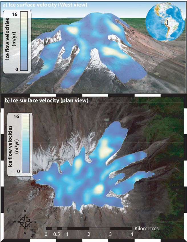
2116                                                   M. Van Wyk de Vries and A. D. Wickert: Glacier Image Velocimetry

locimetry” (PIV). The latter term, particle image velocime-       locity maps are calculated in near real time from Landsat and
try, describes a well-established technique in fluid dynam-       other freely available satellite data sources: GoLIVE using
ics typically involving the use of a high-speed digital camera    PyCorr (Scambos, 2016) and ITS_LIVE using Auto-RIFT
to track the motion of tracers within a fluid in a laboratory     (Gardner et al., 2020).
setting (Buchhave, 1992; Grant, 1997; Raffel et al., 2018).          Table 1 presents a non-exhaustive list of feature-tracking
These ideas were first carried over to the field of glaciol-      software packages. In some circumstances, GIV will not
ogy by Bindschadler and Scambos (1991) and Scambos et al.         be the most suitable feature-tracking tool depending on the
(1992) to evaluate the flow velocity of a portion of an Antarc-   user’s requirements. For example, users who need to manu-
tic ice stream. Since that time, the increasing abundance and     ally perform prior image co-registration (e.g. with airphotos)
availability of imagery has facilitated the expanded use of       may wish to use the built-in workflow in COSI-Corr. The
feature-tracking-based velocimetry techniques. With the re-       objective of the Glacier Image Velocimetry (GIV) toolbox
lease of the full Landsat data archive and launch of Sentinel-    presented here is not to compete with or replace these other
2, 10–30 m pixel resolution imagery of any given location         tools. Rather, GIV aims to provide an easy-to-use, flexible,
is now available at sub-weekly repeat coverage intervals. A       and robust alternative. GIV may be used to derive high spa-
number of studies apply this exceptional archive to map ve-       tial and temporal resolution surface-velocity maps of glaciers
locity fields across the major ice sheets, as well as those of    of all scales. The following section will run through the ba-
many glaciers around the world (Gardner et al., 2018; Millan,     sics of the image-feature-tracking techniques and advances
2019).                                                            built into GIV.
   Prior to the advent of remote sensing, spatially distributed
measurements of glacier flow velocities required lengthy
field campaigns (Meier and Tangborn, 1965; Hooke et al.,          2   Methods and model setup
1989; Chadwell, 1999; Mair et al., 2003). Nowadays full 2D
flow-velocity maps may be readily calculated from a variety       The fundamental idea of feature tracking is based on tech-
of optical- and radar-based satellite imagery (Heid and Kääb,     niques used to co-register images: the properties of two im-
2012b; Fahnestock et al., 2016). For this toolbox we focus on     ages are compared in order to identify the best-fit location of
optical imagery products due to their ease of access, limited     one image within the other (Scambos et al., 1992; Thielicke
need for pre-processing, and high spatial and temporal reso-      and Stamhuis, 2014; Messerli and Grinsted, 2015). In fea-
lution (Drusch et al., 2012; Heid and Kääb, 2012b, a; Kääb        ture tracking, including in GIV, individual images are divided
et al., 2016; Darji et al., 2018).                                into a grid of smaller images (referred to as “chips”). We
   A number of tools exist to derive displacements from           compare each individual chip from the first image (I1) to a
imagery, as partially reviewed by Heid and Kääb (2012a),          surrounding portion within a second image (I2) and find the
Jawak et al. (2018), and Darji et al. (2018). These in-           best matching portion of I2. If no displacement has occurred
clude CARST (Cryosphere and Remote Sensing Toolkit;               between the two images, the best-fitting portion of I2 will
Willis et al., 2018), COSI-corr (Co-registration of Optically     have the same location as the original chip on I1 (excluding
Sensed Images and Correlation; Leprince et al., 2007b),           any georeferencing or distortion-related errors). However, if
AutoRIFT (Autonomous Repeat Image Feature Tracking;               any motion has occurred between the two images, the cor-
Gardner et al., 2018), ImGRAFT (Image Georectification            responding best matching chip within I2 will be displaced
and Feature Tracking; Messerli and Grinsted, 2015), and           relative the original location within I1. We may then deter-
SenDiT (the Sentinel-2 Displacement Toolbox; Nagy and             mine the bulk displacement in pixels between the original I1
Andreassen, 2019; Nagy et al., 2019). CARST contains a            chip and best matching I2 chip. The correlation coefficients
mixture of Python and Bash scripts used to monitor changes        between the original chip and surrounding area within I2 are
in glaciers and includes feature-tracking and ice-elevation-      also calculated. This allows a Gaussian curve to be fit to this
change-monitoring tools (Willis et al., 2018; Zheng et al.,       grid in order to determine the peak location at sub-pixel accu-
2018, 2019a). COSI-Corr is a flexible co-registration and         racy. Repeating this routine for every chip within the original
feature-tracking tool written in IDL, implemented in the          image allows a 2D surface velocity field to be derived.
ENVI GIS package, and initially used for measuring co-               While initially developed for use in laboratory-based fluid
seismic deformation. Auto-RIFT is a Python-based feature-         dynamics, the camera, lighting, and tracer-particle condi-
tracking algorithm (Gardner et al., 2018). ImGRAFT is a           tions were all closely constrained (Grant, 1997; Raffel et al.,
MATLAB-based toolbox for georectifying and feature track-         2018). On glaciers, features change over time as crevasses
ing of ground-based imagery and may also be used on satel-        open and close, snow drifts, and ablation exposes new sur-
lite imagery. SenDiT provides a platform to automatically         faces. In addition, the satellite may acquire imagery from
download and generate velocity maps based on Sentinel-2           slightly different locations and angles with each pass, and
data using a Python interface with bindings to the C- and         lighting conditions depend strongly on the time of day and
Fortran-based imcorr toolbox (Scambos et al., 1992) for           year, as well as degree of shadowing and local weather con-
feature-tracking calculations. In addition, near-global ice ve-   ditions (Berthier et al., 2005; Kääb et al., 2016). This com-

The Cryosphere, 15, 2115–2132, 2021                                                  https://doi.org/10.5194/tc-15-2115-2021
M. Van Wyk de Vries and A. D. Wickert: Glacier Image Velocimetry                                                                        2117

Table 1. Non-exhaustive list of codes and toolboxes that may be used for feature tracking and associated references. For availability, 1 =
fully available, 2 = available but relies on commercial software, and 3 = not available. A spreadsheet with download links is available in the
Supplement.

   Toolbox         Source                              Summary                                                                 Availability
   Auto-RIFT       Gardner et al. (2018)               Python dense feature-tracking package for calculating displacement                1
                                                       from optical or radar imagery. Used for calculating the ITS_LIVE
                                                       global velocity dataset.
   CARST           Zheng et al. (2019a)                Python and bash scripts for feature tracking and ice elevation                    1
                                                       change analysis.
   CIAS            Kääb and Vollmer (2000)             IDL-based correlation software to compute offsets between two im-                 1
                                                       ages.
   Cosi-Corr       Leprince et al. (2007a)             IDL/ENVI-based package for image co-registration and displace-                    2
                                                       ment mapping.
   EMT             Schwalbe and Maas (2017)            Workflow for analysis and feature tracking of time-lapse ground-                  1
                                                       based imagery.
   GIV             This study.                         GUI-based feature-tracking toolbox for glaciology.                                1
   fourDvel        Minchew et al. (2017)               Fortran routine for calculation of 3D velocity fields from geolocated             1
                                                       displacement data.
   ImCorr          Scambos et al. (1992)               C and Fortran package for dense feature tracking of satellite or air-             1
                                                       photo imagery.
   ImGRAFT         Messerli and Grinsted (2015)        MATLAB-based package for georectification of ground-based im-                     2
                                                       agery and feature tracking.
   MatPIV          Sveen (2004)                        MATLAB-based toolbox for pattern matching and particle image                      2
                                                       velocimetry (PIV).
   PIVlab          Thielicke and Stamhuis (2014)       GUI-based MATLAB PIV toolbox.                                                     2
   Pointcatcher    James et al. (2016)                 MATLAB-based toolbox for facilitating manual feature tracking in                  2
                                                       image time series.
   PyCorr          Fahnestock et al. (2016)            Python-based feature-tracking toolbox. Used for calculating the Go-               3
                                                       LIVE global velocity dataset.
   PyTrx           How et al. (2020)                   Python toolbox created for calculating displacements from oblique                 1
                                                       images and time-lapse image series.
   SendIT          Nagy et al. (2019)                  Flexible processing toolbox for retrieval of glacier surface veloci-              1
                                                       ties, based on ImCorr.
   vmap            Shean (2019)                        Ames-Stereo-Pipeline-based image correlator for velocity map gen-                 1
                                                       eration.

plexity raises additional problems in the use of this technique          large datasets. Figure 1 presents the overall model setup and
for deriving glacier velocities and makes it entirely unusable           order of operations.
in some cases (e.g. images too far spaced in time relative
to the speed of the glacier for image pairs to retain any co-            2.1    Model pre-processing
herence). These problems can be mitigated though a combi-
nation of image pre-filtering, comparison between adjacent
                                                                         Prior to running the feature-tracking algorithms, the satellite
velocity maps, and outlier filtering. We also refer readers to
                                                                         images are first loaded into the workspace and filtered. The
Sects. 2 and 4 of Altena (2018) for a detailed discussion on
                                                                         user interface will prompt the user to enter the coordinates
these topics. The Glacier Image Velocimetry toolbox makes
                                                                         of the images (minimum and maximum latitude and longi-
use of these methods, with a particular emphasis on noise re-
                                                                         tude) and to select a given folder in which the images are
duction in individual velocity map outputs through the use of
                                                                         stored. These images can be .png, .jpg, or .geotiff files of the

https://doi.org/10.5194/tc-15-2115-2021                                                          The Cryosphere, 15, 2115–2132, 2021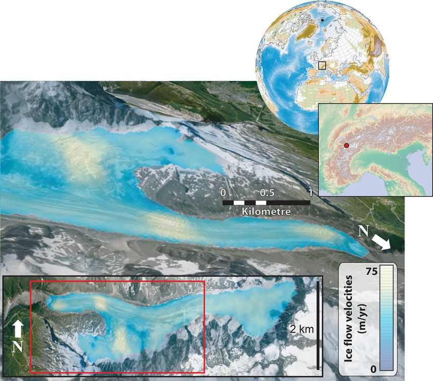
2118                                                        M. Van Wyk de Vries and A. D. Wickert: Glacier Image Velocimetry

Figure 1. Flowchart describing the Glacier Image Velocimetry toolbox design. Names of the code files associated with each step are given
for reference (and are available in the linked Zenodo repository). The feature-tracking step is shown in bold. Note that the source code is
open source but that accessing it is not necessary for running GIV. Users may enter all parameter options into fields in the user interface, with
subsequent steps automatically performed by the toolbox.

area, with each file name being the date of image acquisition              prove image contrast (Sveen, 2004; Thielicke and Stamhuis,
(in yyyymmdd format). In the case of a GeoTIFF input, GIV                  2014; Gardner et al., 2018). We also include a variation of the
will automatically load the geographic information from the                orientation filter (Fitch et al., 2002) named “near anisotropic
input. GIV will then extract the dates from the file names,                orientation filter” (NAOF). We define this filter as follows:
calculate time between images, and load the raw image data
                                                                                  4
into an array for further processing. The user also inputs a                      X
                                                                           If =         cos [arctan 2(Io · αi , Io · R[αi ])] ,              (1)
modified image with glaciers of interest converted to pure                        i=1
white (RGB 255, 255, 255). This image is loaded by GIV
and converted into a binary mask with areas within (1) and                 with If being the filtered image and Io the original im-
outside (0) the computational region. The size and resolution              age, α representing four different convolution matrices ori-
of images are also automatically calculated and resampled to               ented at 45◦ from each other using the eight adjacent pixels,
a common resolution such that images from different satel-                 arctan 2(x, y) representing the four-quadrant arctangent (also
lites may be combined in the same dataset.                                 called the two-argument arctangent), x ×y representing a 2D
   Following this, GIV filters the images according to user-               matrix convolution, and R[x] representing a 90◦ matrix rota-
defined settings. GIV includes a range of filters in order to              tion. This filter works by summing differently angled orien-
reduce the effect of unwanted noise (e.g. clouds and shad-                 tation filters together in order to recover a “pseudo-feature”
ows) and emphasize trackable features (e.g. crevasses, snow-               with the same location as the original feature but with an
drifts, supraglacial debris). In particular we include high-               increased contrast between the feature and the background
pass, Sobel, and Laplacian filter options to emphasize short-              and homogenized magnitude (Fitch et al., 2002; Kobayashi
wavelength features and edges, as well as intensity-capping                and Otsu, 2008). Information on absolute pixel colour mag-
and contrast-limited histogram-equalization filters to im-                 nitude is discarded, with only information on colour gradi-
                                                                           ents preserved. A similar result may be obtained by convolv-

The Cryosphere, 15, 2115–2132, 2021                                                                 https://doi.org/10.5194/tc-15-2115-2021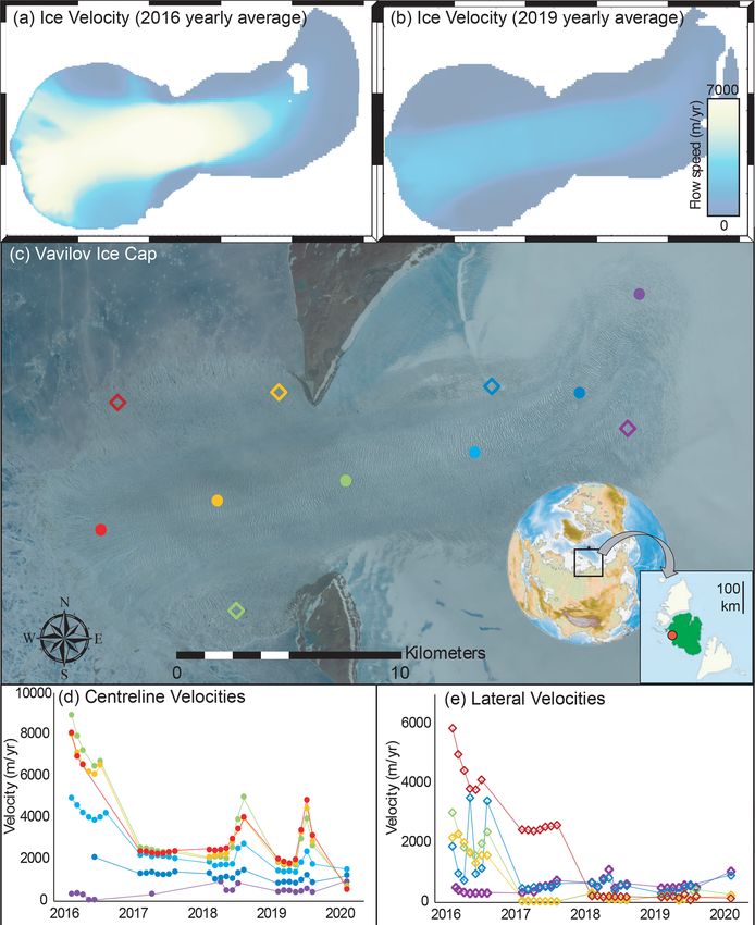
M. Van Wyk de Vries and A. D. Wickert: Glacier Image Velocimetry                                                                           2119

Figure 2. Comparison between raw optical images, band-summed images, and NAOF-filtered images for a clear image (a, d, g), a heavily
shadowed image (b, e, h), and a cloudy image (c, f, i) of Amalia glacier, Patagonia (−50.92◦ S, −73.56◦ W). Note how despite the complexity,
the NAOF images recover a clear and easily traceable feature pattern on the surface of the glacier that is suitable for obtaining velocities. The
shadow line leaves an artefact in (h) but is a marked improvement on the lack of features in the shaded area in (e). Images from Sentinel-2.

ing the original image with a single convolution matrix sum-               be performed in the spatial or frequency domain (Thielicke
ming the four directional filters, but this normalizes all fea-            and Stamhuis, 2014; Altena, 2018). Matching in the spatial
tures to a single magnitude and results in a larger number of              domain (“normalized cross correlation”) may better account
false matches. The NAOF has the advantages of (a) strongly                 for feature distortion or shear and may have a higher ac-
increasing the contrast between features and background;                   curacy (Thielicke and Stamhuis, 2014). Frequency domain
(b) removing contrast differences between clouded, shad-                   methods (“frequency cross correlation”) generally benefit
owed, and clear areas; and (c) preserving feature location                 from a greater computational efficiency as the correlation
and uniqueness. Figure 2 shows examples of how this filter                 matrix is calculated across the whole domain in one oper-
is able to recover features from challenging images. Many                  ation. We implement frequency domain matching in GIV as
glaciated areas remain cloud covered and shadowed for much                 feature distortion is minimal in most glaciers and it has been
of the year, so being able to recover partial velocity fields              found to perform well in prior studies (e.g. Heid and Kääb,
from these images can greatly increase the size of potential               2012a). We refer readers to Thielicke and Stamhuis (2014)
datasets. Note that no amount of filtering can improve certain             and Sect. 4 of Altena (2018) for more details on these topics.
images, such as those in which cloud cover is too thick for                   Frequency cross correlation involves calculating the cor-
the glacier surface to be visible. An evaluation of the quality            relation between the chip and search area in the frequency
of velocity maps derived from different image filters is pro-              domain. This is done by converting both the chip and search
vided in the Supplement (Figs. S1–S16 in the Supplement).                  area to the frequency domain using a fast Fourier transform
These show that NAOF, contrast-limited histogram equaliza-                 (FFT), calculating the pointwise product between these two
tion, and high-pass filtering provide a major improvement                  matrices, and converting the resulting similarity matrix back
over raw imagery.                                                          to the spatial domain with an inverse FFT. This step is re-
                                                                           peated on each chip within the original image and is the most
2.2     Velocity calculations                                              computationally expensive of the entire process.
                                                                              GIV is written in MATLAB. Despite being a high-level
2.2.1    Frequency domain matching                                         interpreted programming language, MATLAB performs FFT
                                                                           calculations using pre-compiled C and Fortran bindings for
The central part of any feature-tracking code involves match-
                                                                           the FFTW library (Frigo and Johnson, 1998, 2005). Due to
ing a small region of one image (chip) with a surrounding re-
                                                                           this being the rate-limiting step in feature-tracking calcula-
gion of a second image (“search area”). The chip is matched
                                                                           tions (> 90 % of computation time in most cases), such code
to the search area through 2D cross correlation, which may

https://doi.org/10.5194/tc-15-2115-2021                                                            The Cryosphere, 15, 2115–2132, 2021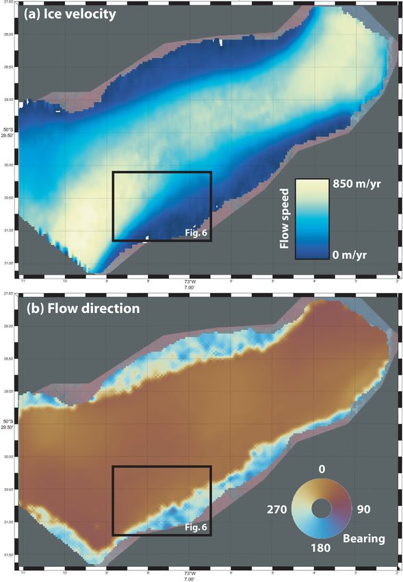
2120                                                        M. Van Wyk de Vries and A. D. Wickert: Glacier Image Velocimetry

                                                                        natively, users may start their own parallel pool with a chosen
                                                                        number of cores. It then decomposes the full sequence of im-
                                                                        age pairs into sub-sequences, each containing a number of
                                                                        image pairs equal to the number of cores. Finally, displace-
                                                                        ments are calculated in parallel on the image pairs within
                                                                        each sub-sequence (each on a different core in the computer).
                                                                        Figure 3 shows the increase in computation speed with num-
                                                                        ber of cores used in different scenarios. This enables large
                                                                        datasets to be processed more rapidly, even on standard lap-
                                                                        top and desktop computers.

                                                                        2.2.3   Single- and multi-pass approaches

                                                                        Displacements may be derived from an image pair either with
                                                                        a single pass across the images or with multiple passes with
                                                                        gradually reducing window sizes (Thielicke and Stamhuis,
                                                                        2014; Raffel et al., 2018). Single-pass methods generally
                                                                        have the advantage of generally being faster at coarse res-
                                                                        olutions and are less at risk of smearing one erroneous
                                                                        value over a larger area. Multi-pass methods update dis-
                                                                        placement estimates over multiple iterations, refining ini-
                                                                        tial coarse-window-size displacement calculations using pro-
                                                                        gressively smaller window sizes. Multi-pass methods com-
                                                                        bine the advantages of better feature matching at large win-
                                                                        dow sizes with the higher spatial resolution of small window
                                                                        sizes. Both methods are integrated into GIV, with a single-
                                                                        pass method based on ImGRAFT (Messerli and Grinsted,
                                                                        2015) and a three-iteration multi-pass algorithm modified
                                                                        from MatPIV (Sveen, 2004). Both functions have been tested
                                                                        in a number of previous studies, with MatPIV being used ex-
                                                                        tensively in fluid-dynamics research (e.g. Sveen and Cowen,
Figure 3. MP = multi-pass; SP = single-pass. Test conducted on          2004; Sveen, 2004; Lee et al., 2017; Oertel and Süfke, 2020).
a 12-image dataset of 10 m resolution, 1.7 million pixel images         An experiment evaluating the difference between a nor-
of Amalia Glacier, Chile, using a Dell XPS 15 laptop (2 × 16 GB         malized cross-correlation algorithm and the multi-pass fre-
DDR4 2666 MHz memory, 6-core Intel i7-8750H 2.20 GHz proces-            quency domain cross correlation in GIV is given in the Sup-
sor). In all cases, parallelization decreases runtime, and going from   plement. We find that the multi-pass frequency domain algo-
one to two cores improves runtime by 1.4–1.9×. Fine-resolution          rithm produces velocity maps with a higher signal to noise
multi-pass runs usually yield the best velocity fields, and (b) shows   ratio than the normalized cross-correlation algorithm across
that these benefit from the largest speed-up when parallelized.         test scenarios with a range of cloud cover.

may be written in MATLAB with few performance issues                    2.2.4   Non-consecutive images
relative to other programming languages.
                                                                        GIV may also calculate velocity maps for pairs of non-
2.2.2   Parallel computing                                              consecutive images, which we refer to as “temporal oversam-
                                                                        pling”, resulting in much larger final datasets. The user in-
As the feature-tracking correlation between two images in-              puts maximum and minimum temporal separations for image
herently requires a large number of FFT and inverse FFT                 pairs, and GIV extracts all suitable pairs, including those that
(IFFT) operations, this step has limited potential for further          are not consecutive. For a dataset of n images, this theoreti-
optimization. Computation time may instead be decreased                 cally enables a total of (n2 − n)/2 image pairs. For example,
by deriving displacement fields from different image pairs              this would produce 19,900 image pairs from a 200-satellite-
in parallel rather than in series. This requires a slightly dif-        image time series. For heavily clouded datasets this also has
ferent code design. First, GIV detects the number of physical           the advantage of increasing the likelihood of forming cloud-
cores on the user’s computer and starts a parallel pool; alter-         free image pairs.

The Cryosphere, 15, 2115–2132, 2021                                                        https://doi.org/10.5194/tc-15-2115-2021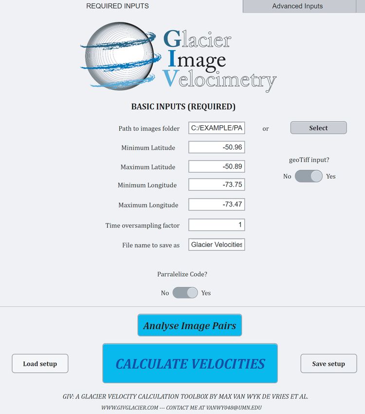
M. Van Wyk de Vries and A. D. Wickert: Glacier Image Velocimetry                                                                       2121

Figure 4. Schematic description of the techniques used to derive monthly velocities. The raw data (a) are combined in a weighted average
to make an initial guess of monthly averages (b). The monthly averages are then used to segment longer time period velocity maps into
their different monthly contributions (c). These are used to recalculate the monthly averages (d). Finally, GIV iterates over steps (b–d) for
a number of times (e.g. 10) provided by user inputs. Note that an estimate may be made for the average velocity in “Month 3” despite this
month having no imagery available.

2.2.5   Velocity map filtering and improvement                           maining values. Secondly, GIV calculates the mean, standard
                                                                         deviation, and median, minimum, and maximum velocities
Apart from some scenarios and positions, such as surges,                 through time at each grid cell in the dataset. It then com-
spring speed-ups, and the margins of ice streams, glacier                pares each individual value to the mean value at that location
velocity gradients vary gradually in both space (low lat-                for the entire dataset. Any values more than 1.5 standard de-
eral velocity gradients) and time (low acceleration). There-             viations away from this mean are considered outliers. This
fore, the accuracy of individual velocity measurements can               process is carried out for the x and y components of veloc-
be evaluated by comparing them to their immediate neigh-                 ity and flow-speed and flow-direction grids, and only values
bours in both space and time. Sudden jumps in space or                   within the threshold for all velocity and flow direction com-
time most likely represent erroneous velocities due to mis-              ponents are conserved. This provides an additional check as
matches within the feature-tracking algorithm. This property             erroneous values are unlikely to coincidentally match both
is used in the GIV toolbox to improve the final velocity maps            the velocity and flow direction. Finally, the entire dataset may
through the following workflow.                                          be smoothed and interpolated in space or time and space ac-
   Firstly, GIV filters each individual velocity map through             cording to the user’s choices. This allows missing values at
user-prescribed limits on velocity and flow direction, as well           one time step to be linearly infilled from neighbouring times.
as outlier detection functions. This finds values that differ by         In addition, the displacement of each image pair may be nor-
more than 50 % from their immediate neighbours (four sur-                malized to the displacement of a user-defined stable ground
rounding cells) and 200 % from the mean of their larger lo-              mask to correct for systematic georeferencing errors.
cal area (25 surrounding cells), removes these outlier values,
and interpolates across these now-empty pixels using the re-

https://doi.org/10.5194/tc-15-2115-2021                                                         The Cryosphere, 15, 2115–2132, 2021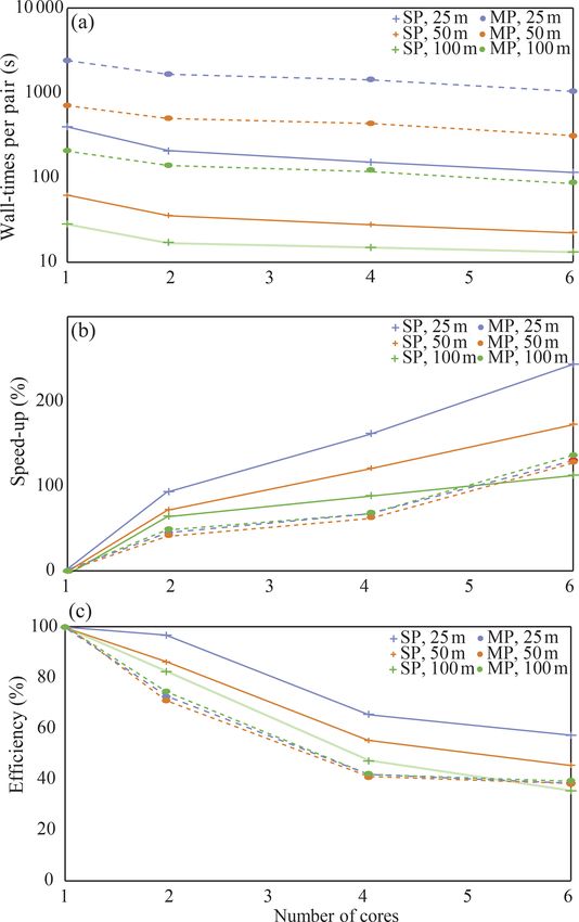
2122                                                    M. Van Wyk de Vries and A. D. Wickert: Glacier Image Velocimetry

2.2.6   Temporal resampling

Variable satellite repeat intervals and the exclusion of en-
tirely clouded or otherwise unusable images lead to unevenly
spaced velocity time series that are more difficult to inter-
pret. In order to reduce this challenge, GIV includes a func-
tion that automatically averages the data and resamples it to
monthly intervals. This is easy when all individual velocity
maps cover periods of less than 1 month and do not overlap
between months but become more complex when they do.
In many cases, image pairs with the shortest lag times (< 7–
10 d) are excluded because displacement over such a short
time may be obscured by offsets due to distortion and/or
georeferencing errors. For the slowest-moving glaciers, this
lower bound may be extended to several weeks or months.
Lag times as long as the available imagery time series may
be used so long as the surface of the glacier retains coherence
in the image pairs.
   GIV can determine monthly values by averaging across all
image pairs that overlap with a given month. However, this
produces an artificially smoothed dataset due to the influence
of velocities measured across the boundaries of months. In
order to make use of longer lag-time pairs, we develop an
iterative strategy for calculating monthly values. In the first
place, GIV takes a weighted mean of all velocities covering
that month to make an initial guess at monthly velocities. The
weighting parameter is determined by the proportion of the
individual map contained within a given month. For instance,
a velocity entirely within 1 month will be weighted 1, while a
velocity spread evenly over 4 months will be weighted 0.25.
This initial estimate is then used to iterate between monthly      Figure 5. Mean flow velocity (m yr−1 ) (a) and direction (de-
averages and raw data values, with raw values covering more        grees) (b) of Glaciar Perito Moreno, Argentina, for the first 3
than 1 month split into monthly values by subtracting the          months of 2020. Figure panels have been automatically generated
previous iteration’s estimate of monthly averages from them        from GIV, labels have been added, and the colour bars moved.
(Fig. 4). This procedure may extract average monthly ve-
locities even for months lacking any images. Outlier detec-
tion and maximum velocity filters are implemented based on         locity and flow-direction maps (Fig. 5). Flow direction maps
user-provided maximum velocity and comparison to neigh-            are plotted with a circular colourmap, and all colour maps
bouring pixels. This prevents noise in the raw data from be-       used are colour-blind friendly based on Crameri et al. (2020)
ing accentuated by the iterations but may also lead to loss        and may be modified according to user preferences. In the
of data if too large a proportion of the initial dataset is in-    following section we will examine some case studies of real
accurate. Due to this limitation, the iterative calculations are   glaciers and scenarios for which this model may be useful.
not adapted for some noisy datasets for which the partial loss
of temporal resolution by weighted averaging will be prefer-       3   Results and examples
able. Monthly averaging is performed as a post-processing
step and so may be repeated without the need to recalculate        Ice velocity measurements supply essential information for
any raw velocity maps. Time series may also be generated           studies of glacier dynamics, thickness, subglacial hydrology,
from the raw data if monthly averaging is not desirable.           and mass balance. With its GUI-based inputs and potential
                                                                   for parallelization, GIV can calculate a monthly velocity field
2.2.7   Georeferencing and plotting                                for any glacier around the world with only a few hours of
                                                                   work. As such, it may also be run alongside field-based ex-
As a final step, GIV will automatically georeference the ve-       peditions in order to understand the current conditions of the
locity grids and save .geotiff files to the user’s computer. The   glacier and aid in instrumentation positioning.
toolbox also contains mapping tools that allow for the au-
tomatic generation of publication-quality images of the ve-

The Cryosphere, 15, 2115–2132, 2021                                                   https://doi.org/10.5194/tc-15-2115-2021
M. Van Wyk de Vries and A. D. Wickert: Glacier Image Velocimetry 2123
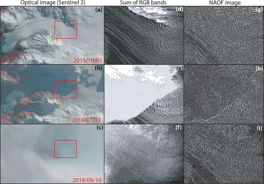
Figure 6. (a) Position of a point on Glaciar Perito Moreno (PM) with the time for three different starting locations within 2 km of the
glacier’s southern margin. At PM1, ice speeds reach 800 m yr−1 , and any equipment will be rapidly displaced. At PM3 ice-flow speeds
are < 100 m yr−1 and oriented towards the valley edge. (b) Identical plot for two points on Glaciar Europa (EU). Any equipment installed at
EU1 will be displaced several kilometres and lost to calving in less than 6 months. The inlay shows an outline of the Southern Patagonian
Icefield (SPI) with the locations of the two glaciers. Imagery © Google Earth.
We present four case studies. The first is of Glaciar Per- 3.1 Field campaign support: Glaciar Perito Moreno
ito Moreno (50.48◦ S, 73.11◦ W), where we use GIV to de- and the Southern Patagonian Icefield
termine the displacement of automated ablation stakes in
conjunction with fieldwork in Spring 2020. The second is
A team from the University of Minnesota installed three au-
Glacier d’Argentière (45.95◦ N, 06.97◦ E), a small and well-
tomated weather stations and three automated ablation stakes
studied valley glacier located in the French Alps. The third
near the southern flank of Glaciar Perito Moreno in order
is Vavilov Ice Cap (79.32◦ N, 94.34◦ E), located on Octo-
to better understand the local conditions of this glacier and
ber Revolution Island in the Arctic Ocean off the mainland
construct temperature-index and energy-balance models for
Russian coast, whose western outlet glacier is now surging.
glacier ablation. We installed the automated ablation stakes,
Here we evaluate GIV against published results (Zheng et al.,
based on designs by Wickert (2014) and Wickert et al. (2019)
2019b) using another image-based ice velocity tool, CARST
and tested by Saberi et al. (2019) and Armstrong and An-
(Zheng et al., 2019a). Finally, we compute ice-flow veloc-
derson (2020), for 20 d between 23 February and 14 March,
ities across the glaciers on Volcán Chimborazo (01.45◦ S,
2020. In slow-moving glaciers, ice flow may be largely ne-
78.82◦ W) in Ecuador.
glected when considering equipment recovery. In rapidly
flowing glaciers such as Perito Moreno, however, it may be
https://doi.org/10.5194/tc-15-2115-2021 The Cryosphere, 15, 2115–2132, 2021
2124                                                    M. Van Wyk de Vries and A. D. Wickert: Glacier Image Velocimetry

Figure 7. Perspective view of mean flow velocities of Glacier d’Argentière, France, over the period March 2019–March 2020. Imagery is
from © Google Earth, and scale is for near margin of glacier.

relevant to consider the movement of the glacier when plan-          3.2   Valley-glacier velocity distribution: Glacier
ning equipment recovery. This is particularly relevant where               d’Argentière
intense crevassing makes both access and visibility difficult.
Figure 6 shows how different positioning decisions may in-           In order to evaluate the effectiveness of GIV on smaller
fluence ease of recovery: ablation stakes installed in position      glaciers, we calculate a velocity field for a well-studied val-
PM1 will move tens of metres towards the glacier calving             ley glacier in the Mont Blanc massif, Glacier d’Argentière
front in less than a month, whereas stakes in position PM3           (Benoit et al., 2015). We download 1-year worth of Sentinel-
will move less than 5 m towards the glacier flank. In our sur-       2 data (March 2019–March 2020), containing over 1000
vey, stakes were installed around position PM3 for ease of           image pairs. These images are then used to derive a 25 m
access.                                                              resolution mean ice velocity map, shown in Fig. 7. The
   Figure 6b also presents the case of Glaciar Europa, which         sparsity of features transverse to flow direction on Glacier
drains the adjacent portion of the Southern Patagonian Ice-          d’Argentière make it difficult for feature-tracking methods to
field in Chile. We also derived the mean velocity field of           calculate velocities. Nevertheless, the resulting flow-velocity
this glacier over the past 3 years using Sentinel-2 imagery          map is comparable to those derived using a SPOT satel-
(195 image pairs). GIV velocity measurements reveal that             lite image pair from 2003 (Berthier et al., 2005; Rabatel
the central portion of Glaciar Europa at its outlet flows nearly     et al., 2018), synthetic-aperture radar (SAR), and ground-
10 000 m yr−1 . If an ablation stake were installed in this area     based photogrammetry (Benoit et al., 2015) and a different
(point EU1), it would be displaced almost half a kilometre           feature-tracking routine based on a modified version of amp-
over the course of a 20 d survey. If it were instead placed at       cor (Millan et al., 2019). The velocity map highlights acceler-
an alternative location 1 km to the west (EU2), it would be          ated ice flow at the terminus icefall and on the steep tributary
displaced only 20 m in the same time period. This is an ex-          glacier to the south-west of the main trunk (Fig. 7). Main-
treme case, and the flow speeds of most glaciers are orders of       trunk velocities are on the order of 45–70 m yr−1 , slightly
magnitude slower, but it showcases the potential importance          slower than SPOT values from Berthier et al. (2005) but in
of deriving glacier surface velocity fields for the success of a     line with values from Benoit et al. (2015). Our values repre-
glaciological field campaign.                                        sent the mean over an entire year, including the slower winter

The Cryosphere, 15, 2115–2132, 2021                                                      https://doi.org/10.5194/tc-15-2115-2021
M. Van Wyk de Vries and A. D. Wickert: Glacier Image Velocimetry                                                                       2125

Figure 8. (a, b) 100 m resolution annual mean velocities for the western outlet glacier of Vavilov Ice Cap. (c) A 2019 Sentinel-2 image
showing the main features of this outlet and the locations used to derive monthly time series. (d, e) Monthly resolution velocity time series
along the glacier centreline and flanks using Sentinel-2 imagery.

velocities not captured by Berthier et al. (2005). It is also pos-          Vavilov Ice Cap is a 1700 km3 glacier on October Rev-
sible that glacier thinning has reduced its flow velocity, but           olution Island in the Severnaya Zemlya archipelago located
our data are not sufficient to evaluate this.                            in the Russian high arctic (Bassford et al., 2006). Until the
                                                                         2010s, Vavilov Ice Cap exhibited surface velocities of only
3.3   Vavilov Ice Cap dynamics                                           a few tens of metres per year, typical of many cold-based
                                                                         high-arctic ice masses. In 2013, a large portion of the marine-
Arctic land-ice melt, including both the Greenland Ice Sheet             terminating western flank surged, with the ice front reach-
and all Arctic glaciers, has contributed more than 20 mm                 ing more than 10 km beyond its prior grounding line by
to global sea level rise since the 1970s (Box et al., 2018).             2016 (Willis et al., 2018; Zheng et al., 2019b). This sud-
Most of these large glaciers remain remote and difficult to ac-          den shift in ice behaviour was not accompanied by any dra-
cess, and high spatial and temporal resolution surface veloc-            matic climatic shift, and the exact triggers are a matter of
ity maps provide one important tool to assess their response             active debate (Willis et al., 2018, and references therein).
to changing environmental conditions.                                    Willis et al. (2018) proposed that the dramatic acceleration
                                                                         is related to the glacier overriding weak marine sediments

https://doi.org/10.5194/tc-15-2115-2021                                                         The Cryosphere, 15, 2115–2132, 2021
2126 M. Van Wyk de Vries and A. D. Wickert: Glacier Image Velocimetry Figure 9. Comparison between the velocity maps of Zheng et al. (2019b) for Vavilov Ice Cap (Pair037_20170506_20170522) and results from GIV (May 2017 average). (a) Difference map, corresponding to the velocity minus GIV velocity from Zheng et al. (2019b), (b) percent- age of the total velocity this difference represents (absolute value of the difference shown in (a) divided by GIV velocity), and (c) histogram of the difference values. The mean difference between the two velocity maps is less than 20 m yr−1 or less than 1 % of the total velocity for much of the area. in the Kara Sea, which can deform easily and substantially spring and early summer rates and rapidly decaying (Fig. 7d). increase ice velocity. The glacier margin is also no longer Within the newly formed western frontal lobe, extruded be- frozen to bedrock, leading to the associated removal of re- yond the prior grounding line, flow has concentrated into a sistive stresses at the ice front (Willis et al., 2018). Rapid single branch with well-developed shear margins separating ice flow initiates a set of internal feedbacks to further in- a central region with rapid ice flow from slow-moving lateral crease ice velocity, including strain softening of the ice it- portions of the glacier (Zheng et al., 2019b). self, shear heating that produces meltwater capable of reduc- Extraction of high-resolution ice velocities in this region ing the effective normal stress of the ice and hence its fric- using GIV confirms the findings of Willis et al. (2018) and tion against the bed, and potential infiltration of this water Zheng et al. (2019b) that the western portion of Vavilov has into the bed material, increasing its deformability (Sevestre entered into a new fast-flow regime. The late summer veloc- and Benn, 2015; Willis et al., 2018, and references therein). ity peaks in both 2018 and 2019 may shed some light on the With no direct data on subglacial conditions prior to or dur- driving forces behind this acceleration if associated changes ing the surge, the exact processes involved remain difficult to in climatic, ice surface, or ice basal conditions are identified. determine. We may, however, monitor surface ice velocities Ongoing monitoring will help to determine whether a similar to examine the ongoing changes in ice kinematics. peak occurs in subsequent years, and this can be performed Optical satellite imagery from Vavilov Ice Cap is avail- in near real time using GIV. able only for summer months (March to September) due to We compare our GIV-derived results against a velocity darkness during the high-latitude boreal winter. We use GIV map of the front of the western outlet glacier generated by to derive a 100 m resolution ice velocity map of a 365 km2 Zheng et al. (2019b) using CARST (Zheng et al., 2019a). area of the western flank of the glacier using all Sentinel-2 Zheng et al. (2019b) generated their velocity map based imagery from 2016 to 2020. Figure 8a and b present two av- on a single Landsat 8 pair dated 6 and 22 May 2017. We erage yearly velocity maps for the apex of the surge in 2016 compared the ice-surface velocity magnitude calculated from and in 2019. Figure 8d and e presents time series of monthly this pair to the May 2017 average velocity map generated velocities over the period from March 2016 to March 2020 from Sentinel-2 imagery using GIV through the approach at the locations shown in Fig. 8c. described above. We georeferenced the two velocity maps Velocities of the centreline points converge over the time using the glacier margins and other notable features. The dif- period considered: although the velocities near the ice front ference map (Fig. 9a) displays the highest amplitude anoma- decrease from the 2016 peak (red, orange, and green cir- lies along the margins of the central high-velocity band. cles), velocities of regions most distant from the coast show Differences between the GIV- and CARST-derived veloc- a steady increase (purple points). The central portion of this ity maps are normally distributed, with a mean difference of newly formed outlet glacier shows distinct late-summer ac- −16 m yr−1 (Fig. 9c). This mean difference is ≤ 1 % of the celerations in both 2018 and 2019, reaching around double its speed across the majority of the glacier surface (Fig. 9b). In The Cryosphere, 15, 2115–2132, 2021 https://doi.org/10.5194/tc-15-2115-2021
M. Van Wyk de Vries and A. D. Wickert: Glacier Image Velocimetry 2127
this region of the glacier surface, the annual variability in ice-
surface velocities is on the order of several hundred metres
per year (Fig. 8d and e), and this difference may result from
the slightly different dates covered or differing image reso-
lutions (10 m for Sentinel-2 compared to 15–30 m for Land-
sat). The high-magnitude difference bands on either side of
the fast-moving central region may also result in whole or in
part from georeferencing errors in GIV, in CARST, or in our
work to georeference these two velocity maps to one another.
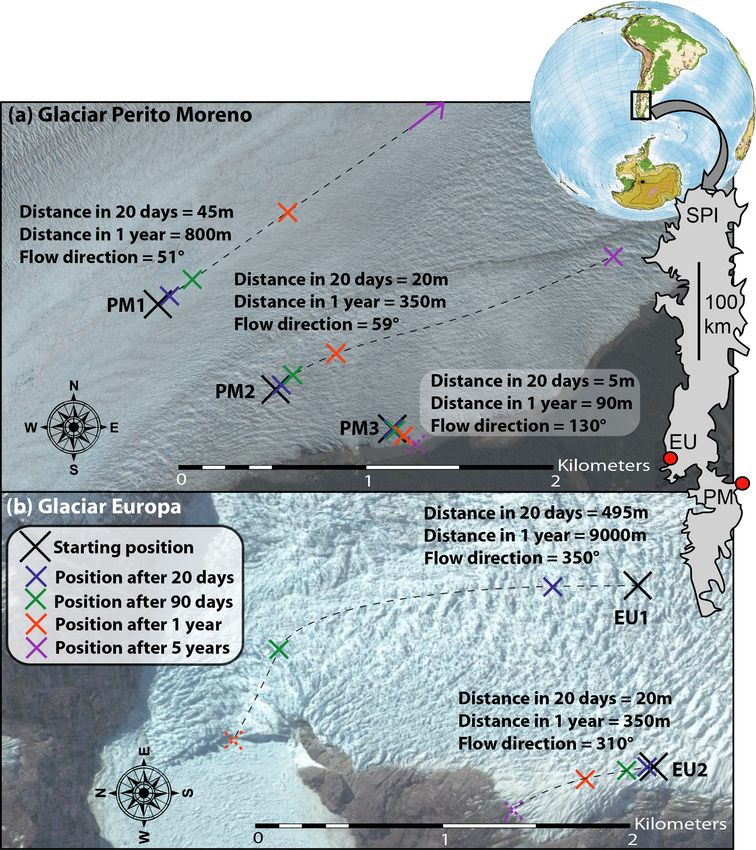
3.4 Ice velocity of a small tropical glacier: Chimborazo
Many tropical glaciers have limited to no ice-flow data from
direct field measurements (Thompson et al., 2011). These are
important water sources to millions of people (Bury et al.,
2011; Chevallier et al., 2011; La Frenierre and Mark, 2017).
Vergara et al. (2007) estimated the economic cost of glacier
retreat on water use to be in the hundreds of millions of
US dollars and the impact on Peru’s electrical utility to be
∼ 1.5 billion. High-resolution estimates of ice velocity pro-
vide information on glacier state and can contribute to prac-
tical decision-making in the tropical Andes.
Chimborazo is a 6268 m high stratovolcano in Ecuador
covered with 17 glaciers. On Chimborazo’s north-eastern
flank, glacier meltwater drives nearly all of the discharge
variability, and the disappearance of the prominent Reschre-
iter Glacier could decrease the discharge of the watershed’s Figure 10. Ice-surface-velocity map for the Chimborazo glaciers
calculated with GIV. Imagery © Google Earth and Sentinel-2.
outlet stream by up to 50 % (Saberi et al., 2019). Due to its
high elevation and steep slopes that are unstable in regions of
recent ice retreat, the glaciers on Chimborazo are difficult to
survey (Saberi et al., 2019). No field measurements of glacier or more (Fig. 3). This makes velocity-field calculations with
surface velocity have been conducted. hundreds to tens of thousands of image pairs practical on reg-
Chimborazo poses challenges to feature-tracking-based ular computers. The inclusion of “temporal oversampling”
ice velocimetry as its glaciers are small, regularly feature- allows much larger datasets to be generated than via simple
poor or snow covered, very slow moving, and cloud covered consecutive image comparison; a dataset of 100 images may
for large parts of the year. The velocity limitations are mit- in fact include several thousand usable image pairs. We com-
igated by using only images with large temporal separation bine methodological advances in feature tracking and image
(acquisition dates more than 6 months apart). GIV is also processing from both geoscience and engineering toolboxes
well suited for extracting velocities from partially clouded and develop new filtering techniques to improve the quality
imagery. We run GIV on the full Sentinel-2 dataset, which is of the final surface-velocity maps. GIV provides a rapid and
comprised of 91 individual partially or fully cloud-free im- easy-to-use interface (shown in Fig. 11) and a user manual
ages. These were cropped to Chimborazo, resulting in 3062 and may also be of use to communities who would not gen-
image pairs separated by at least 6 months. Resultant ice erally be involved with glacier remote sensing (Van Wyk de
velocities for each pair were corrected for the mean dis- Vries, 2021a, b).
placement of a stable, non-glaciated region surrounding the GIV is easily learned and is not computationally time-
glaciers. Results are shown in Fig. 10. consuming, and the results derived with it are easy to re-
produce. GIV allows users to modify image-processing and
feature-tracking parameters based on their expert knowledge
4 Discussion and conclusions of particular glaciers without the need for specific compu-
tational knowledge. GIV may be run either directly through
These four examples underline GIV’s flexibility, ease of use, MATLAB functions, through a MATLAB graphical user in-
and ability to rapidly process large datasets for calculating terface (Van Wyk de Vries, 2021a), or as an independent
ice velocities in a range of environments. Most regular lap- desktop app that may be run with no MATLAB license (Van
top and desktop computers now include at least four cores, Wyk de Vries, 2021b). GIV has been tested and successfully
which GIV uses to speed up calculations by a factor of 2 run on Windows, Mac, and Linux operating systems.
https://doi.org/10.5194/tc-15-2115-2021 The Cryosphere, 15, 2115–2132, 20212128 M. Van Wyk de Vries and A. D. Wickert: Glacier Image Velocimetry
Figure 11. Main graphical user interface for GIV showing the main input fields. This interface may either be run through MATLAB or as an
independent desktop app with no licensing requirements.
In summary, GIV is a versatile, GUI-based, and fully par- Code availability. MATLAB code for GIV may be downloaded
allelized toolbox that enables the rapid calculation of glacier from https://github.com/MaxVWDV/glacier-image-velocimetry
velocity fields from satellite imagery. GIV builds upon re- (last access: 24 April 2021, Van Wyk de Vries, 2021a).
cent improvements in optical satellite imagery availability The GIV stand-alone app may be downloaded from
and resolution to extract high temporal and high spatial reso- https://github.com/MaxVWDV/glacier-image-velocimetry-app
(last access: 24 April 2021, Van Wyk de Vries, 2021b). Both
lution velocity maps, and it uses novel and pre-existing filters
include a user manual and an example dataset.
to optimize the quality of these velocity maps. GIV has been
successfully tested on a wide range of environments, includ-
ing small valley glaciers (Glacier d’Argentière, France), trop-
Data availability. All the velocity maps presented in this paper are
ical glaciers (Volcán Chimborazo, Ecuador), and large outlet derived from Sentinel-2 imagery, which may be freely accessed on-
glaciers (Glaciar Perito Moreno, Argentina, and outflow from line. Specific example datasets and information on how to repro-
Vavilov Ice Cap, Russia). We show that ice velocity datasets duce our results are included in the GIV GitHub repository and user
are versatile and may be used to complement field campaigns manual.
and study the dynamics of large and small glaciers. Source
code and pre-compiled binary executables for GIV are avail-
able from Van Wyk de Vries (2021a) and Van Wyk de Vries
(2021b).
The Cryosphere, 15, 2115–2132, 2021 https://doi.org/10.5194/tc-15-2115-2021M. Van Wyk de Vries and A. D. Wickert: Glacier Image Velocimetry 2129
Supplement. The supplement related to this article is available on- Benoit, L., Dehecq, A., Pham, H.-T., Vernier, F., Trouvé, E.,
line at: https://doi.org/10.5194/tc-15-2115-2021-supplement. Moreau, L., Martin, O., Thom, C., Pierrot-Deseilligny,
M., and Briole, P.: Multi-method monitoring of Glacier
d’Argentière dynamics, Ann. Glaciol., 56, 118–128,
Author contributions. MVWdV and ADW planned the project. https://doi.org/10.3189/2015AoG70A985, 2015.
MVWdV wrote the code and ran the examples. MVWdV and ADW Berthier, E., Vadon, H., Baratoux, D., Arnaud, Y., Vincent, C., Feigl,
wrote and edited the manuscript. K. L., Rémy, F., and Legrésy, B.: Surface motion of mountain
glaciers derived from satellite optical imagery, Remote Sens.
Environ., 95, 14–28, https://doi.org/10.1016/j.rse.2004.11.005,
Competing interests. The authors declare that they have no conflict 2005.
of interest. Bindschadler, R. A. and Scambos, T. A.: Satellite-Image-Derived
Velocity Field of an Antarctic Ice Stream, Science, 252, 242–
246, https://doi.org/10.1126/science.252.5003.242, 1991.
Bottomley, J. T.: Flow of Viscous Materials–A Model Glacier, Na-
Acknowledgements. Maximillian Van Wyk de Vries was supported
ture, 21, 159–159, https://doi.org/10.1038/021159a0, 1879.
by a University of Minnesota College of Science and Engineering
Box, J. E., Colgan, W. T., Wouters, B., Burgess, D. O., O’Neel, S.,
fellowship. Ben Popken assisted with early testing of GIV. Emi Ito,
Thomson, L. I., and Mernild, S. H.: Global sea-level contribu-
Kelly MacGregor, Jeff La Frenierre, Matias Romero, Shanti B. Pen-
tion from Arctic land ice: 1971–2017, Environ. Res. Lett., 13,
prase, Jabari Jones, and Kerry L. Callaghan provided comments
125 012, https://doi.org/10.1088/1748-9326/aaf2ed, 2018.
on this manuscript. David Carchipulla helped improve image-
Buchhave, P.: Particle image velocimetry–status and trends, Exp.
download workflows. Conversations about feature tracking with
Therm. Fluid Sci., 5, 586–604, https://doi.org/10.1016/0894-
Whyjay Zheng, Shashank Bhushan, Will Kochtitzky, and David
1777(92)90016-X, 1992.
Shean have helped refine the ideas in this paper and in GIV’s code.
Bury, J. T., Mark, B. G., McKenzie, J. M., French, A., Baraer, M.,
We acknowledge Ted Scambos and two anonymous referees for
Huh, K. I., Zapata Luyo, M. A., and Gómez López, R. J.: Glacier
thoughtful reviews which improved both the manuscript and the as-
recession and human vulnerability in the Yanamarey watershed
sociated toolbox. We further thank editor Harry Zekollari for de-
of the Cordillera Blanca, Peru, Climatic Change, 105, 179–206,
tailed suggestions which were valuable for fine-tuning our text and
https://doi.org/10.1007/s10584-010-9870-1, 2011.
figures. This material is based upon work supported by the National
Chadwell, C. D.: Reliability analysis for design of stake networks
Science Foundation under grant no. EAR-1714614, coordinated by
to measure glacier surface velocity, J. Glaciol., 45, 154–164,
lead PI Maria Beatrice Magnani.
https://doi.org/10.3189/S0022143000003130, 1999.
Chevallier, P., Pouyaud, B., Suarez, W., and Condom, T.: Cli-
mate change threats to environment in the tropical Andes:
Financial support. This research has been supported by the United glaciers and water resources, Reg. Environ. Change, 11, 179–
States National Science Foundation (grant no. EAR-1714614). 187, https://doi.org/10.1007/s10113-010-0177-6, 2011.
Crameri, F., Shephard, G. E., and Heron, P. J.: The misuse of
colour in science communication, Nat. Commun., 11, 5444,
Review statement. This paper was edited by Harry Zekollari and https://doi.org/10.1038/s41467-020-19160-7, 2020.
reviewed by Ted Scambos and two anonymous referees. Darji, S., Shah, R. D., Oza, S., and Bahuguna, I. M.: Inter-
Comparison of Various Feature Tracking Tools Deriving Glacier
Ice Velocity, Int. J. Sci. Res. Rev., 7, 422–429, 2018.
Davies, B. J. and Glasser, N. F.: Accelerating shrink-
References age of Patagonian glaciers from the Little Ice Age
(∼ AD 1870) to 2011, J. Glaciol., 58, 1063–1084,
Altena, B.: Observing change in glacier flow by using optical satel- https://doi.org/10.3189/2012JoG12J026, 2012.
lites, PhD thesis, available at: https://www.duo.uio.no/handle/ Deeley, R. M. and Parr, P. H.: XVI. The Hintereis Glacier, The Lon-
10852/61747 (last access: 24 April 2021), 2018. don, Edinburgh, and Dublin Philosophical Magazine and Journal
Altena, B., Scambos, T., Fahnestock, M., and Kääb, A.: Extract- of Science, 27, 153–176, 1914.
ing recent short-term glacier velocity evolution over south- Drusch, M., Del Bello, U., Carlier, S., Colin, O., Fernandez,
ern Alaska and the Yukon from a large collection of Landsat V., Gascon, F., Hoersch, B., Isola, C., Laberinti, P., Marti-
data, The Cryosphere, 13, 795–814, https://doi.org/10.5194/tc- mort, P., Meygret, A., Spoto, F., Sy, O., Marchese, F., and
13-795-2019, 2019. Bargellini, P.: Sentinel-2: ESA’s Optical High-Resolution Mis-
Armstrong, W. H. and Anderson, R. S.: Ice-marginal lake hydrol- sion for GMES Operational Services, Remote Sens. Environ.,
ogy and the seasonal dynamical evolution of Kennicott Glacier, 120, 25–36, https://doi.org/10.1016/j.rse.2011.11.026, 2012.
Alaska, J. Glaciol., 66, 699–713, 2020. Fahnestock, M., Scambos, T., Moon, T., Gardner, A., Ha-
Bassford, R. P., Siegert, M. J., Dowdeswell, J. A., Oerlemans, ran, T., and Klinger, M.: Rapid large-area mapping of ice
J., Glazovsky, A. F., and Macheret, Y. Y.: Quantifying the flow using Landsat 8, Remote Sens. Environ., 185, 84–94,
Mass Balance of Ice Caps on Severnaya Zemlya, Russian High https://doi.org/10.1016/j.rse.2015.11.023, 2016.
Arctic. I: Climate and Mass Balance of the Vavilov Ice Cap, Fitch, A., Kadyrov, A., Christmas, W., and Kittler, J.: Ori-
Arct. Antarct. Alp. Res., 38, 1–12, https://doi.org/10.1657/1523- entation Correlation, in: Procedings of the British Ma-
0430(2006)038[0013:QTMBOI]2.0.CO;2, 2006.
https://doi.org/10.5194/tc-15-2115-2021 The Cryosphere, 15, 2115–2132, 20212130 M. Van Wyk de Vries and A. D. Wickert: Glacier Image Velocimetry chine Vision Conference 2002, pp. 11.1–11.10, British Ma- Data, Proceedings, 2, 341, https://doi.org/10.3390/ecrs-2-05154, chine Vision Association, Cardiff, 2–5 September 2002, 2018. https://doi.org/10.5244/C.16.11, 2002. Kamb, B. and LaChapelle, E.: Direct Observation of the Mecha- Forbes, J. D.: The Glacier Theory, google-Books-ID: nism of Glacier Sliding Over Bedrock, J. Glaciol., 5, 159–172, wPoTAAAAQAAJ, 1840. https://doi.org/10.3189/S0022143000028756, 1964. Forbes, J. D.: XII. Illustrations of the viscous theory of Kääb, A. and Vollmer, M.: Surface Geometry, Thickness glacier motion. – Part I. Containing experiments on the Changes and Flow Fields on Creeping Mountain Per- flow of plastic bodies, and observations on the phenomena mafrost: Automatic Extraction by Digital Image Analysis, Per- of lava streams, Philos. T. R. Soc. Lond., 136, 143–155, mafrost Periglac., 11, 315–326, https://doi.org/10.1002/1099- https://doi.org/10.1098/rstl.1846.0013, 1846. 1530(200012)11:43.0.CO;2-J, 2000. Fowler, A.: Weertman, Lliboutry and the develop- Kääb, A., Winsvold, S. H., Altena, B., Nuth, C., Nagler, T., ment of sliding theory, J. Glaciol., 56, 965–972, and Wuite, J.: Glacier Remote Sensing Using Sentinel-2. https://doi.org/10.3189/002214311796406112, 2010. Part I: Radiometric and Geometric Performance, and Ap- Frigo, M. and Johnson, S.: FFTW: an adaptive software ar- plication to Ice Velocity, Remote Sens.-bASEL, 8, 598, chitecture for the FFT, in: Proceedings of the 1998 IEEE https://doi.org/10.3390/rs8070598, 2016. International Conference on Acoustics, Speech and Sig- Kobayashi, T. and Otsu, N.: Image Feature Extraction Using Gradi- nal Processing, ICASSP ’98 (Cat. No.98CH36181), vol. 3, ent Local Auto-Correlations, in: Computer Vision – ECCV 2008, pp. 1381–1384, IEEE, Seattle, WA, USA, 15 May 1998, edited by: Forsyth, D., Torr, P., and Zisserman, A., Lecture Notes https://doi.org/10.1109/ICASSP.1998.681704, 1998. in Computer Science, vol. 5302, Springer, Berlin, Heidelberg, Frigo, M. and Johnson, S.: The Design and Im- https://doi.org/10.1007/978-3-540-88682-2_27, 2008. plementation of FFTW3, P. IEEE, 93, 216–231, La Frenierre, J. and Mark, B. G.: Detecting Patterns of Cli- https://doi.org/10.1109/JPROC.2004.840301, 2005. mate Change at Volcán Chimborazo, Ecuador, by Inte- Gardner, A., Fahnestock, M., and Scambos, T.: ITS_LIVE Regional grating Instrumental Data, Public Observations, and Glacier Glacier and Ice Sheet Surface Velocities, National Snow and Ice Change Analysis, Ann. Am. Assoc. Geogr., 107, 979–997, Data Center, https://doi.org/10.5067/6II6VW8LLWJ7, 2020. https://doi.org/10.1080/24694452.2016.1270185, 2017. Gardner, A. S., Moholdt, G., Scambos, T., Fahnstock, M., Lee, R. M., Yue, H., Rappel, W.-J., and Losert, W.: Data from: Infer- Ligtenberg, S., van den Broeke, M., and Nilsson, J.: In- ring single cell behavior from large-scale epithelial sheet migra- creased West Antarctic and unchanged East Antarctic ice dis- tion patterns, Digital Repository at the University of Maryland, charge over the last 7 years, The Cryosphere, 12, 521–547, https://doi.org/10.13016/M2855R, 2017. https://doi.org/10.5194/tc-12-521-2018, 2018. Leprince, S., Ayoub, F., Klinger, Y., and Avouac, J.-P.: Grant, I.: Particle image velocimetry: A re- Co-Registration of Optically Sensed Images and Cor- view, P. I. Mech. Eng. C-J. Mec., 211, 55–76, relation (COSI-Corr): an operational methodology for https://doi.org/10.1243/0954406971521665, 1997. ground deformation measurements, in: 2007 IEEE Inter- Heid, T. and Kääb, A.: Evaluation of existing image matching meth- national Geoscience and Remote Sensing Symposium, pp. ods for deriving glacier surface displacements globally from op- 1943–1946, IEEE, Barcelona, Spain, 23–28 July 2007, tical satellite imagery, Remote Sens. Environ., 118, 339–355, https://doi.org/10.1109/IGARSS.2007.4423207, 2007a. https://doi.org/10.1016/j.rse.2011.11.024, 2012a. Leprince, S., Barbot, S., Ayoub, F., and Avouac, J.-P.: Automatic Heid, T. and Kääb, A.: Repeat optical satellite images reveal and Precise Orthorectification, Coregistration, and Subpixel Cor- widespread and long term decrease in land-terminating glacier relation of Satellite Images, Application to Ground Deforma- speeds, The Cryosphere, 6, 467–478, https://doi.org/10.5194/tc- tion Measurements, IEEE T. Geosci. Remote, 45, 1529–1558, 6-467-2012, 2012b. https://doi.org/10.1109/TGRS.2006.888937, 2007b. Hooke, R. L., Calla, P., Holmlund, P., Nilsson, M., and Stroeven, Mair, D., Willis, I., Fischer, U. H., Hubbard, B., Nienow, P., A.: A 3 Year Record of Seasonal Variations in Surface and Hubbard, A.: Hydrological controls on patterns of sur- Velocity, StorglaciÄren, Sweden, J. Glaciol., 35, 235–247, face, internal and basal motion during three “spring events”: https://doi.org/10.3189/S0022143000004561, 1989. Haut Glacier d’Arolla, Switzerland, J. Glaciol., 49, 555–567, How, P., Hulton, N. R. J., Buie, L., and Benn, D. I.: https://doi.org/10.3189/172756503781830467, 2003. PyTrx: A Python-Based Monoscopic Terrestrial Pho- Meier, M. F. and Tangborn, W. V.: Net Budget and Flow of togrammetry Toolset for Glaciology, Front. Earth Sci., 8, South Cascade Glacier, Washington, J. Glaciol., 5, 547–566, https://doi.org/10.3389/feart.2020.00021, 2020. https://doi.org/10.3189/S0022143000018608, 1965. Howat, I. M., Porter, C., Smith, B. E., Noh, M.-J., and Morin, P.: Messerli, A. and Grinsted, A.: Image georectification and feature The Reference Elevation Model of Antarctica, The Cryosphere, tracking toolbox: ImGRAFT, Geosci. Instrum. Method. Data 13, 665–674, https://doi.org/10.5194/tc-13-665-2019, 2019. Syst., 4, 23–34, https://doi.org/10.5194/gi-4-23-2015, 2015. James, M. R., How, P., and Wynn, P. M.: Pointcatcher software: Millan, R.: Ice thickness and bed elevation of the Patagonian Ice- analysis of glacial time-lapse photography and integration with fields [Data set], Dryad, https://doi.org/10.7280/d11q17, 2019. multitemporal digital elevation models, J. Glaciol., 62, 159–169, Millan, R., Mouginot, J., Rabatel, A., Jeong, S., Cusican- https://doi.org/10.1017/jog.2016.27, 2016. qui, D., Derkacheva, A., and Chekki, M.: Mapping Sur- Jawak, S. D., Kumar, S., Luis, A. J., Bartanwala, M., Tummala, S., face Flow Velocity of Glaciers at Regional Scale Using a and Pandey, A. C.: Evaluation of Geospatial Tools for Generating Multiple Sensors Approach, Remote Sens.-Basel, 11, 2498, Accurate Glacier Velocity Maps from Optical Remote Sensing https://doi.org/10.3390/rs11212498, 2019. The Cryosphere, 15, 2115–2132, 2021 https://doi.org/10.5194/tc-15-2115-2021
You can also read