Linking global terrestrial CO2 fluxes and environmental drivers: inferences from the Orbiting Carbon Observatory 2 satellite and terrestrial ...
←
→
Page content transcription
If your browser does not render page correctly, please read the page content below
Atmos. Chem. Phys., 21, 6663–6680, 2021
https://doi.org/10.5194/acp-21-6663-2021
© Author(s) 2021. This work is distributed under
the Creative Commons Attribution 4.0 License.

Linking global terrestrial CO2 fluxes and environmental drivers:
inferences from the Orbiting Carbon Observatory 2 satellite and
terrestrial biospheric models
Zichong Chen1 , Junjie Liu2 , Daven K. Henze3 , Deborah N. Huntzinger4 , Kelley C. Wells5 , Stephen Sitch6 ,
Pierre Friedlingstein7 , Emilie Joetzjer8 , Vladislav Bastrikov9 , Daniel S. Goll10 , Vanessa Haverd11 , Atul K. Jain12 ,
Etsushi Kato13 , Sebastian Lienert14 , Danica L. Lombardozzi15 , Patrick C. McGuire16 , Joe R. Melton17 ,
Julia E. M. S. Nabel18 , Benjamin Poulter19 , Hanqin Tian20 , Andrew J. Wiltshire21 , Sönke Zaehle22 , and
Scot M. Miller1
1 Department    of Environmental Health and Engineering, Johns Hopkins University, Baltimore, MD, USA
2 Jet Propulsion Laboratory, California Institute of Technology, Pasadena, CA, USA
3 Department of Mechanical Engineering, University of Colorado Boulder, Boulder, CO, USA
4 School of Earth and Sustainability, Northern Arizona University, Flagstaff, AZ, USA
5 Department of Soil, Water, and Climate, University of Minnesota Twin Cities, St. Paul, MN, USA
6 College of Life and Environmental Sciences, University of Exeter, Exeter, UK
7 College of Engineering, Mathematics and Physical Sciences, University of Exeter, Exeter, UK
8 Centre National de Recherche Météorologique, Unité mixte de recherche 3589 Meteo-France/CNRS,

42 Avenue Gaspard Coriolis, 31100 Toulouse, France
9 Laboratoire des Sciences du Climat et de l’Environnement, Institut Pierre-Simon Laplace, CEA-CNRS-UVSQ,

CE Orme des Merisiers, 91191 Gif-sur-Yvette CEDEX, France
10 Université Paris-Saclay, CEA-CNRS-UVSQ, LSCE/IPSL, Gif-sur-Yvette, France
11 CSIRO Oceans and Atmosphere, G.P.O. Box 1700, Canberra, ACT 2601, Australia
12 Department of Atmospheric Sciences, University of Illinois, Urbana, IL, USA
13 Institute of Applied Energy (IAE), Minato-ku, Tokyo 105-0003, Japan
14 Climate and Environmental Physics, Physics Institute and Oeschger Centre for Climate Change Research,

University of Bern, Bern, Switzerland
15 Terrestrial Sciences Section, Climate and Global Dynamics, National Center for Atmospheric Research, Boulder, CO, USA
16 Department of Meteorology, Department of Geography and Environmental Science, National Centre for Atmospheric

Science, University of Reading, Reading, UK
17 Climate Research Division, Environment and Climate Change Canada, Victoria, BC, Canada
18 Max Planck Institute for Meteorology, Hamburg, Germany
19 NASA Goddard Space Flight Center, Biospheric Sciences Laboratory, Greenbelt, MD, USA
20 International Center for Climate and Global Change Research, School of Forestry and Wildlife Sciences,

Auburn University, 602 Duncan Drive, Auburn, AL, USA
21 Met Office Hadley Centre, FitzRoy Road, Exeter EX1 3PB, UK
22 Max Planck Institute for Biogeochemistry, P.O. Box 600164, Hans-Knöll-Str. 10, 07745 Jena, Germany

Correspondence: Zichong Chen (zchen74@jhu.edu)

Received: 25 March 2020 – Discussion started: 24 April 2020
Revised: 11 December 2020 – Accepted: 28 March 2021 – Published: 4 May 2021

Published by Copernicus Publications on behalf of the European Geosciences Union.
6664                                                                            Z. Chen et al.: Global CO2 fluxes from space

Abstract. Observations from the Orbiting Carbon Observa-           sinks (e.g., Eldering et al., 2017; Liu et al., 2017; Crowell
tory 2 (OCO-2) satellite have been used to estimate CO2            et al., 2019; Palmer et al., 2019; Byrne et al., 2020a).
fluxes in many regions of the globe and provide new insight           Recent advances in OCO-2 retrievals from the NASA
into the global carbon cycle. The objective of this study is       ACOS science team have led to widespread reductions in
to infer the relationships between patterns in OCO-2 obser-        observation errors (e.g., O’Dell et al., 2018). Reducing the
vations and environmental drivers (e.g., temperature, precip-      errors in satellite observations of CO2 is critical for under-
itation) and therefore inform a process understanding of car-      standing CO2 sources and sinks using inverse modeling, as
bon fluxes using OCO-2. We use a multiple regression and           even small biases in the observations can have an impact on
inverse model, and the regression coefficients quantify the        the CO2 flux estimate (e.g., Chevallier et al., 2007, 2014;
relationships between observations from OCO-2 and envi-            Feng et al., 2016; Miller et al., 2018). For example, Miller
ronmental driver datasets within individual years for 2015–        et al. (2018) evaluated the extent to which OCO-2 retrievals
2018 and within seven global biomes. We subsequently com-          can detect patterns in biospheric CO2 fluxes and found that
pare these inferences to the relationships estimated from 15       an early version of the OCO-2 retrievals (version 7) is only
terrestrial biosphere models (TBMs) that participated in the       equipped to provide accurate flux constraints across very
TRENDY model inter-comparison. Using OCO-2, we are                 large continental or hemispheric regions; by contrast, in a
able to quantify only a limited number of relationships be-        follow-up paper, Miller and Michalak (2020) revisited satel-
tween patterns in atmospheric CO2 observations and patterns        lite capabilities in light of recently improved OCO-2 re-
in environmental driver datasets (i.e., 10 out of the 42 re-       trievals, and the authors argued that new OCO-2 retrievals
lationships examined). We further find that the ensemble of        can be used to constrain CO2 fluxes for more detailed regions
TBMs exhibits a large spread in the relationships with these       (i.e., for seven global biomes).
key environmental driver datasets. The largest uncertainty in         A further challenge is to use these new global satellite
the models is in the relationship with precipitation, particu-     datasets to evaluate and improve process-based estimates of
larly in the tropics, with smaller uncertainties for temperature   the global carbon cycle provided by terrestrial biospheric
and photosynthetically active radiation (PAR). Using obser-        models (TBMs). TBMs have become an integral tool for un-
vations from OCO-2, we find that precipitation is associated       derstanding regional- and global-scale carbon dynamics and
with increased CO2 uptake in all tropical biomes, a result         for predicting future carbon cycling under changing climate.
that agrees with half of the TBMs. By contrast, the relation-      With that said, existing TBMs show large uncertainties in
ships that we infer from OCO-2 for temperature and PAR are         carbon flux estimates at multiple spatial and temporal scales
similar to the ensemble mean of the TBMs, though the results       – at regional and seasonal scales (e.g., Peng et al., 2014;
differ from many individual TBMs. These results point to the       King et al., 2015), at global and inter-annual scales (e.g., Piao
limitations of current space-based observations for inferring      et al., 2020), and in historical and future projections (e.g.,
environmental relationships but also indicate the potential to     Friedlingstein et al., 2006; Huntzinger et al., 2017).
help inform key relationships that are very uncertain in state-       One approach to inform TBM development is to estimate
of-the-art TBMs.                                                   flux totals using atmospheric observations and compare those
                                                                   totals against TBMs – to inform the magnitude, seasonal-
                                                                   ity, or spatial distribution of fluxes (e.g., King et al., 2015;
                                                                   Bastos et al., 2018). A more challenging approach is to esti-
1   Introduction                                                   mate the relationships between CO2 fluxes and environmen-
                                                                   tal drivers using atmospheric observations and compare those
Over the past decade, the field of space-based CO2 moni-           relationships directly to the relationships in TBMs. We define
toring has undergone a rapid evolution. The sheer number           the term “environmental drivers” as any meteorological vari-
of CO2 -observing satellites has greatly increased, includ-        ables or characteristics of the physical environment that can
ing GOSAT/GOSAT-2 (Kuze et al., 2009; Nakajima et al.,             be modeled or measured and may correlate with net ecosys-
2012), TanSat (Yang et al., 2018), and OCO-2/OCO-3 (Crisp,         tem exchange (NEE). Several studies have shown that these
2015; Eldering et al., 2019). This expanding observing sys-        types of comparisons are feasible using in situ atmospheric
tem provides atmospheric CO2 observations broadly across           observations (e.g., Dargaville et al., 2002; Forkel et al., 2016;
the globe, making it possible to estimate the distribution and     Gourdji et al., 2008, 2012; Piao et al., 2013, 2017; Wang
magnitude of CO2 fluxes in many regions that have sparse           et al., 2014; Fang and Michalak, 2015; Shiga et al., 2018;
in situ surface atmospheric CO2 monitoring (e.g., the trop-        Wang et al., 2020). Among other studies, Fang and Micha-
ics and the Southern Hemisphere). For example, the OCO-            lak (2015) used in situ atmospheric CO2 observations across
2 satellite, launched in July 2014, provides ∼ 65 000 obser-       North America and an inverse modeling framework to probe
vations per day that pass quality screening (Eldering et al.,      the relationships between NEE and environmental drivers;
2017); this dense, global set of OCO-2 observations, com-          the authors compared these relationships directly to those in-
bined with inverse modeling techniques, has been used to           ferred from several TBMs and found that TBMs have rea-
constrain regional- and continental-scale CO2 sources and          sonable skill in representing the relationship with shortwave

Atmos. Chem. Phys., 21, 6663–6680, 2021                                              https://doi.org/10.5194/acp-21-6663-2021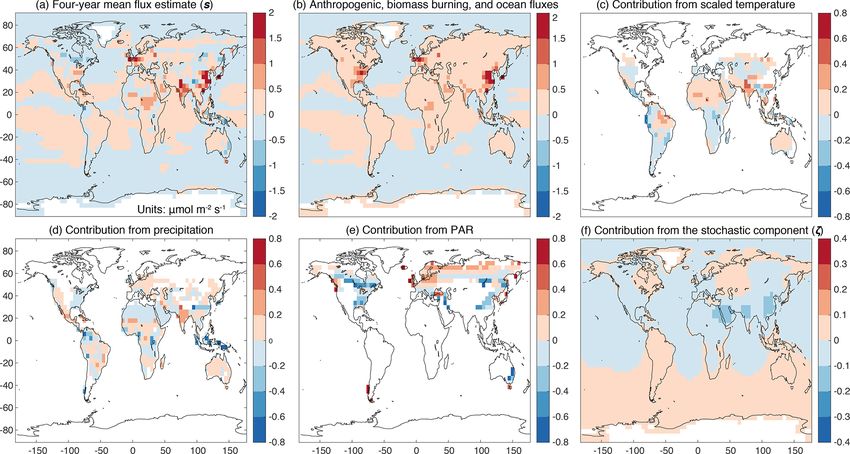
Z. Chen et al.: Global CO2 fluxes from space 6665
radiation but show weak performance in describing relation- 2 Methods
ships with other drivers like water availability. Similarly,
Shiga et al. (2018) used tower-based atmospheric CO2 ob- 2.1 Overview
servations to explore regional interannual variability (IAV)
in NEE across North America and found that TBMs disagree We quantify the relationships between CO2 observations
on the dominant regions responsible for IAV; this disagree- from OCO-2 and environmental driver datasets for different
ment can be linked to differing sensitivities of CO2 fluxes regions of the globe using a top-down regression framework
to environmental drivers within the TBMs. At an even longer and a GIM. We cannot directly observe the relationships be-
temporal scale, Wang et al. (2014) employed the atmospheric tween CO2 fluxes and environmental driver datasets. With
CO2 growth rate record from Mauna Loa, Hawaii, USA, and that said, an overarching idea of this study is that these rela-
the South Pole for five decades to explore the sensitivity of tionships manifest in atmospheric CO2 observations, and we
the global CO2 growth rate to tropical temperature; the au- can quantify at least some of these relationships using obser-
thors found that existing TBMs do not capture the observed vations from OCO-2 and a weighted multiple regression. The
sensitivity of the growth rate to tropical climatic variability, coefficients estimated as part of the regression relate patterns
implying a limited ability of these TBMs in representing the in atmospheric CO2 observations to patterns in the environ-
impact of drought and warming on tropical carbon dynamics. mental driver datasets.
More recently, a handful of studies have shown that it is As part of this analysis, we also explore differences in the
possible to tease out relationships between CO2 fluxes and estimated environmental relationships (i.e., regression coef-
environmental drivers using global satellite observations of ficients) among different years and different biomes. To this
CO2 (e.g., Liu et al., 2017; Byrne et al., 2020b). For example, end, we estimate separate regression coefficients for each
Liu et al. (2017) used observations from OCO-2 to disentan- of seven different global biomes, and we estimate sepa-
gle the environmental processes related to flux anomalies in rate coefficients for each individual year of the study pe-
tropical regions during the 2015–2016 El Niño. Byrne et al. riod (2015–2018). Hence, each coefficient estimated here
(2020b) assimilated in situ and GOSAT observations of at- represents the relationship between OCO-2 observations and
mospheric CO2 and an inverse model framework and found an environmental driver dataset across an entire year and a
contrasting environmental sensitivities of IAV in CO2 fluxes global biome. Miller and Michalak (2020) explored when
between western and eastern temperate North America. and where current OCO-2 observations can be use to detect
The goal of this study is to use atmospheric CO2 obser- variability in surface CO2 fluxes, and the authors argue that,
vations from OCO-2 to quantify the relationships between in most seasons, the satellite can be used to constrain fluxes
spatiotemporal patterns in CO2 fluxes and patterns in en- from seven large biome-based regions – hence the choice of
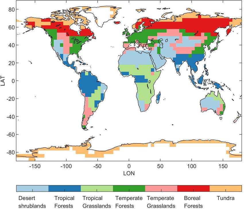
vironmental driver datasets. We conduct this analysis for the seven biomes used in this study (Fig. 1).
years 2015–2018 and focus on relationships that manifest We first conduct this analysis using CO2 observations from
across an individual year and individual biome. We specif- OCO-2. We then conduct a parallel analysis using the out-
ically quantify the relationships using a top-down regres- puts of 15 terrestrial biosphere models (TBMs) from the
sion framework and a geostatistical inverse model (GIM). We TRENDY model inter-comparison project (v8). The goal of
then compare the relationships inferred using OCO-2 obser- this step is to compare the environmental relationships (i.e.,
vations against those inferred from 15 state-of-the-art TBMs regression coefficients) that we infer from OCO-2 against the
from the TRENDY model comparison project (v8, https: regression coefficients that we estimate from numerous state-
//sites.exeter.ac.uk/trendy (last access: 28 October 2020); see of-the-art TBMs. We can then identify any similarities or dif-
Table S1 for a full list of TBMs; Sitch et al., 2015; Friedling- ferences between the TBMs and inferences using OCO-2 ob-
stein et al., 2019). The primary objectives of this analysis servations. We specifically analyze TRENDY model outputs
are threefold: (1) evaluate what kinds of environmental re- for years 2015–2018, the same years as the OCO-2 analysis
lationships we can infer using current satellite observations described above. To conduct this analysis, we generate syn-
from OCO-2, (2) assess where and when TBMs do and do thetic OCO-2 observations using each of the 15 TBMs and
not show consensus on the relationships between CO2 fluxes using an atmospheric transport model. We then run the mul-
and salient environmental drivers, and (3) compare the rela- tiple regression on these synthetic observations. This setup
tionships inferred from OCO-2 against those inferred from mirrors that of Fang and Michalak (2015) and creates an
TBMs with the goal of informing and improving TBM de- apples-to-apples comparison between the TBMs and OCO-2
velopment. observations; in each case, we use atmospheric observations
(either real or synthetic) and use the same set of equations to
estimate the regression coefficients.
The multiple regression used in this study has the follow-
ing mathematical form (e.g., Fang and Michalak, 2015):
z = h(Xβ + ζ ) + , (1)
https://doi.org/10.5194/acp-21-6663-2021 Atmos. Chem. Phys., 21, 6663–6680, 2021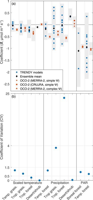
6666                                                                               Z. Chen et al.: Global CO2 fluxes from space

Figure 1. The seven biome-based regions aggregated from a world biome map in Olson et al. (2001).

where z (n × 1) is a vector of real or synthetic CO2 observa-        tions (e.g., Mueller et al., 2010; Yadav et al., 2010), and to
tions from OCO-2, X (m × p) is a matrix of environmental             infer relationships between atmospheric CO2 observations
driver datasets (described in Sect. 2.2), and β (p × 1) rep-         and environmental driver datasets (e.g., Gourdji et al., 2012;
resents the regression coefficients that are estimated as part       Fang et al., 2014; Fang and Michalak, 2015; Piao et al.,
of the regression. Each column of X represents a different           2013, 2017; Rödenbeck et al., 2018).
environmental driver dataset for a specific biome in a spe-             The equations above require an atmospheric transport
cific year. Note that we estimate all of the coefficients for the    model (h()). We use the forward GEOS-Chem model (ver-
different environmental drivers and different biomes simul-          sion v9-02; http://www.geos-chem.org, last access: 28 Oc-
taneously in the regression model. In addition, ζ (m×1) rep-         tober 2020) in this study, and we further use wind fields
resents patterns in the fluxes that cannot be described by the       from the Modern-Era Retrospective Analysis for Research
environmental driver datasets, and these values are unknown.         and Applications (MERRA-2) to drive atmospheric transport
This component of the fluxes is also commonly referred to as         within GEOS-Chem (Gelaro et al., 2017). The GEOS-Chem
the stochastic component and is discussed in Sect. 2.5. h() is       simulations used here have a global spatial resolution of 4◦
an atmospheric transport model (described later in this sec-         latitude by 5◦ longitude and therefore are best able to capture
tion) that relates surface CO2 fluxes (Xβ + ζ ) to the atmo-         broad, regional spatial patterns in atmospheric CO2 .
spheric CO2 observations, and  (n × 1) is a vector of errors
in the OCO-2 observations and/or in the atmospheric model.           2.2   Environmental driver datasets
The statistical properties of these errors are estimated before
running the regression (described in Sect. 2.4).                     We estimate the relationships between OCO-2 observations
   Note that this framework assumes linear relationships be-         (either real or synthetic) and environmental driver datasets
tween the environmental driver datasets and the OCO-2 ob-            drawn from commonly used meteorological reanalysis. We
servations. Numerous existing studies have used linear mod-          specifically consider the following driver datasets as pre-
els to approximate relationships with environmental driver           dictor variables in the multiple regression: 2 m air tempera-
datasets. For example, studies have used linear models to            ture, precipitation, photosynthetically active radiation (PAR),
compare the relationships between CO2 fluxes and envi-               downwelling shortwave radiation, and specific humidity.
ronmental driver datasets in TBMs (e.g., Huntzinger et al.,             We also include a nonlinear function of 2 m air tempera-
2011), to infer these relationships using eddy flux observa-         ture as an environmental driver dataset in the regression (re-
                                                                     ferred to hereafter as scaled temperature; plotted in Fig. S1

Atmos. Chem. Phys., 21, 6663–6680, 2021                                                https://doi.org/10.5194/acp-21-6663-2021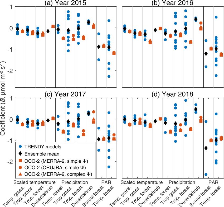
Z. Chen et al.: Global CO2 fluxes from space                                                                                  6667

and described in detail in Supplement Sect. S3). Numerous          dex) in the present study. Rather, the focus of this study is to
existing studies show that the relationship between tempera-       explore environmental drivers of CO2 fluxes and not remote
ture and photosynthesis has a different sign depending upon        sensing proxies for CO2 fluxes. Also note that we standard-
the temperature range; at sufficiently warm temperatures, an       ize (i.e., normalize) each of the environmental driver datasets
increase in temperature yields a decrease in photosynthesis        within each biome and each year before running the regres-
(e.g., Baldocchi et al., 2017). The scaled temperature func-       sion, as has been done in several previous GIM studies (e.g.,
tion considered here can account for those differences, and        Gourdji et al., 2012; Fang and Michalak, 2015). This step
we find that this function yields a better model–data fit in       means that all of the estimated regression coefficients (β)
the regression analysis than using temperature alone. The          have the same units, are independent of the original units on
scaled temperature function used here is from the Vegeta-          the environmental driver data, and can be directly compared
tion Photosynthesis and Respiration Model (VPRM) (Ma-              to one another.
hadevan et al., 2008) and describes the nonlinear relationship
between temperature and photosynthesis (Raich et al., 1991).       2.3   Model selection
The function is shaped like an upside-down parabola (shown
in Fig. S1). Furthermore, this type of nonlinear temperature       We use model selection to decide which environmental driver
function has been commonly used in existing TBMs (e.g.,            datasets to include in the analysis of the OCO-2 observa-
Heskel et al., 2016; Luus et al., 2017; Dayalu et al., 2018;       tions and in the analysis of each TBM using synthetic ob-
Chen et al., 2019).                                                servations. Model selection ensures that the environmental
   The environmental driver datasets described above are           driver datasets in the regression (X) do not overfit the avail-
drawn from the Climatic Research Unit (CRU) and Japanese           able OCO-2 data (z). The inclusion of additional environ-
reanalysis (JRA) meteorology product (CRUJRA; Harris,              mental driver datasets or columns in X will always improve
2019). We use environmental driver data from CRUJRA be-            the model–data fit in the regression, but the inclusion of too
cause it is the same product used to generate the TRENDY           many driver datasets in X can overfit the regression to avail-
model estimates. All flux outputs from TRENDY are pro-             able OCO-2 data and result in unrealistic coefficients (β)
vided at a monthly temporal resolution, so we input monthly        (e.g., Zucchini, 2000). In addition, model selection indicates
meteorological variables from CRUJRA into the regression           which relationships with environmental drivers we can con-
framework. Furthermore, we regrid the environmental driver         fidently constrain and which we cannot given current OCO-2
datasets to a 4◦ latitude by 5◦ longitude spatial resolution be-   observations (e.g., Miller et al., 2018). In this study, we im-
fore inputting these datasets into the regression. This spatial    plement a type of model selection known as the Bayesian
resolution matches the resolution of the atmospheric trans-        information criterion (BIC) (Schwarz et al., 1978), and var-
port simulations used in this study (described in Sect. 2.1).      ious forms of the BIC have been implemented in numerous
The regression coefficients therefore quantify the relation-       recent atmospheric inverse modeling studies (e.g., Gourdji
ships between OCO-2 observations and patterns in environ-          et al., 2012; Miller et al., 2013, 2018; Fang and Michalak,
mental driver datasets that manifest at this spatial and tem-      2015; Miller and Michalak, 2020). Using the BIC, we score
poral resolution.                                                  different combinations of environmental driver datasets that
   We subsequently rerun the regression analysis using en-         could be included in X based on how well each combination
vironmental driver datasets drawn from a second meteoro-           helps reproduce either the real or synthetic OCO-2 observa-
logical product. Estimates of environmental driver data like       tions (z, Eq. 1). We specifically use an implementation of
temperature or precipitation can vary among meteorological         the BIC from Miller et al. (2018) and Miller and Michalak
models, and these differences among models are a source of         (2020) that is designed to be computationally efficient for
uncertainty in the estimated regression coefficients. Hence,       very large satellite datasets. The BIC scores in this imple-
the use of a second meteorological product can at least par-       mentation are calculated using the following equation:
tially account for these uncertainties. We specifically rerun      BIC = L + p ln n∗ ,                                          (2)
the regression analysis using environmental driver datasets
drawn from MERRA-2. We choose MERRA-2 because it is                where L is the log likelihood of a particular combination of
a commonly used, global reanalysis product from the NASA           environmental driver datasets (i.e., columns of X), p is the
Global Modeling and Assimilation Office (GMAO). Further-           number of environmental driver datasets in a particular com-
more, we use wind fields from MERRA-2 to drive all atmo-           bination, and n∗ is the effective number of independent ob-
spheric transport model simulations in this study (described       servations. This last variable accounts for the fact that not all
in Sect. 2.1), so the use of MERRA-2 for the environmental         atmospheric observations are independent, and the model–
driver datasets in the regression creates consistency with the     data residuals can exhibit spatially and temporally correlated
wind fields in the atmospheric model simulations that sup-         errors (Miller et al., 2018). For all simulations here, we use
port the regression.                                               an estimate of n∗ for the v9 OCO-2 observations from Miller
   Note that we do not include any remote sensing indices          and Michalak (2020). The first component of Eq. 2 (L) re-
(e.g., solar-induced chlorophyll fluorescence or leaf area in-     wards combinations that are a better fit to the OCO-2 ob-

https://doi.org/10.5194/acp-21-6663-2021                                            Atmos. Chem. Phys., 21, 6663–6680, 2021
6668                                                                             Z. Chen et al.: Global CO2 fluxes from space

servations (z), whereas the second component of Eq. (2)             that describes ζ (the patterns in the fluxes that cannot be de-
(p ln n∗ ) penalizes models with a greater number of columns        scribed by the environmental driver datasets). This formula-
to prevent overfitting. The best combination of environmen-         tion is more complete because it fully accounts for the resid-
tal drivers for X is the combination that receives the lowest       uals between z and Xβ. However, it is extremely computa-
BIC score. Miller et al. (2018) describes this implementation       tionally intensive to estimate the coefficients (β) using this
of the BIC in greater detail, including the specific setup and      complex formulation of 9. We cannot explicitly formulate
equations.                                                          this more complex version of 9 due to its large size and the
   Note that we run model selection for the OCO-2 data              number of atmospheric model simulations (h()) that would
and rerun model selection for each set of synthetic OCO-2           be required. As a result, we find the solution to Eq. (3) using
datasets generated using each TBM. As a result, we some-            this complex version of 9 by iteratively minimizing the cost
times select different environmental driver datasets for the        function for a geostatistical inverse model (GIM) (Sects. 2.5
analysis using different TBMs. This setup parallels that of         and S1), a process that takes approximately 2 weeks for each
Huntzinger et al. (2011) and Fang and Michalak (2015).              year of model simulations in the setup used here.
Furthermore, we use the same set of environmental driver               We use both the simple and complex formulations of 9
datasets in each year of the study period (e.g., 2015–2018),        when analyzing the real OCO-2 observations. Both the sim-
a setup that parallels existing GIM studies that use multiple       ple and complex formulations of 9 yield similar estimates
years of atmospheric observations (e.g., Shiga et al., 2018).       for the coefficients β, as discussed in the Results and discus-
We estimate different regression coefficients (β) for each          sion (Sect. 3.2). When analyzing the 15 TRENDY models,
year of the study period, but the actual environmental driver       we only use the simple, diagonal formulation of 9 – because
datasets included in the regression do not change from one          of the prohibitive computational costs that would be required
year to the next. An environmental driver dataset is either se-     to run the more complex approach for all 15 TRENDY mod-
lected to be included for all years in a specific biome (based      els.
on the BIC scores) or it is not used in any year of the analysis.      Note that we estimate the values of Q, the covariance ma-
                                                                    trix that describes ζ , using an approach known as restricted
2.4    Statistical model for estimating the coefficients (β)        maximum likelihood (RML) estimation (e.g., Mueller et al.,
                                                                    2008; Gourdji et al., 2008, 2010, 2012). In the Supplement,
Once we have chosen a set of environmental driver datasets          we discuss the structure of Q in detail, describe RML, and
using model selection, we estimate the coefficients (β) that        compare the estimated parameters for Q against existing
relate the real or synthetic OCO-2 observations to these en-        studies.
vironmental datasets (e.g., Gourdji et al., 2012; Fang and
Michalak, 2015):                                                    2.5   Statistical model for estimating CO2 fluxes using
                                                                          OCO-2 observations
β̂ = (h(X)T 9 −1 h(X))−1 h(X)T 9 −1 z,                       (3)

where 9 (n×n) is a covariance matrix that describes model–          To complement the analysis described above, we take an ad-
data residuals (discussed at the end of this section). Further-     ditional step for the real OCO-2 observations of estimating
more, the uncertainties in these estimated coefficients can         ζ , patterns in the fluxes that cannot be described by the envi-
also be estimated using a linear equation (e.g., Gourdji et al.,    ronmental driver datasets, also known as the stochastic com-
2008; Fang and Michalak, 2015):                                     ponent of the fluxes (Eq. 1). This step thereby creates a com-
                                                                    plete estimate of CO2 fluxes using OCO-2 observations. This
Vβ̂ = (h(X)T 9 −1 h(X))−1 ,                                  (4)    additional step accomplishes two goals. First, the fluxes in ζ
                                                                    can reveal flux anomalies or patterns that are too complex to
where Vβ̂ is a p × p covariance matrix.                             quantify using a linear combination of environmental vari-
   We test out two different formulations for the covariance        ables and/or can indicate the strengths and shortfalls of the
matrix 9 to evaluate the sensitivity of the results to the as-      regression. Second, by estimating all components of the CO2
sumptions made about the covariance matrix parameters. In           fluxes (Xβ and ζ ), we can better evaluate our inferences us-
one set of simulations, we model 9 as a diagonal matrix.            ing OCO-2 against independent, ground-based observations
The diagonal values characterize model–data errors (), es-         of CO2 . This independent evaluation is important because
timated for the version 9 retrievals from the recent OCO-2          OCO-2 observations and the atmospheric transport model
model inter-comparison project (e.g., Crowell et al., 2019).        (i.e., GEOS-Chem) can contain errors.
The values have an average standard deviation of 0.98 ppm               We generate a complete estimate of the CO2 fluxes (Xβ +
and range from 0.29 to 4.8 ppm. In a second set of simu-            ζ ) by minimizing the cost function for a GIM (e.g., Kitanidis,
lations, we use a more complex and more complete formu-             1986; Michalak et al., 2004; Miller et al., 2020). We describe
lation of 9: 9 = h(h(Q)T ) + R (e.g., Fang and Michalak,            this process in detail in Supplement Sect. S1. This process
2015), where R (n × n) characterizes the model–data errors          requires two covariance matrices (R and Q), and we use the
(described above), and Q (m × m) is a covariance matrix             same parameters for these covariance matrices as described

Atmos. Chem. Phys., 21, 6663–6680, 2021                                               https://doi.org/10.5194/acp-21-6663-2021
Z. Chen et al.: Global CO2 fluxes from space 6669
above in Sect. 2.4. Note that for the setup here, we estimate ζ
at a spatial resolution of 4◦ latitude by 5◦ longitude to match
that of GEOS-Chem, and we estimate ζ at a daily tempo-
ral resolution to better account for sub-monthly variability in
CO2 fluxes. Also note that minimizing the GIM cost function
yields the same estimate for the coefficients (β) as in Eq. (3),
provided that the covariance matrices in the GIM cost func-
tion and in Eq. (3) are identical. The Supplement Sect. S1
and Miller et al. (2020) describe the process of minimizing
the GIM cost function in greater detail.
2.6 Analysis using real observations from OCO-2
For analysis using OCO-2 observations, we employ 10 s av-
erages of the version 9 OCO-2 observations (e.g., Crowell
et al., 2019) and include both land nadir- and land-glint-mode
retrievals. Recent retrieval updates have greatly reduced bi-
ases that previously existed between land nadir and land
glint observations (O’Dell et al., 2018). Moreover, Miller
and Michalak (2020) evaluated the impact of these updated
OCO-2 retrievals on the terrestrial CO2 flux constraint in dif-
ferent regions of the globe; the authors found that the in-
clusion of both land nadir and land glint retrievals yielded
a stronger constraint on CO2 fluxes relative to using only a
single observation type.
We also include a column of X in all simulations using real
OCO-2 observations to account for anthropogenic emissions,
ocean fluxes, and biomass burning. This column includes
anthropogenic emissions from the Open-Data Inventory for
Anthropogenic Carbon dioxide (ODIAC) (Oda et al., 2018),
ocean fluxes from NASA Estimating the Circulation and Cli-
mate of the Ocean (ECCO) Darwin (Carroll et al., 2020),
and biomass burning fluxes from the Global Fire Emissions
Database (GFED) (Randerson et al., 2018). We estimate a
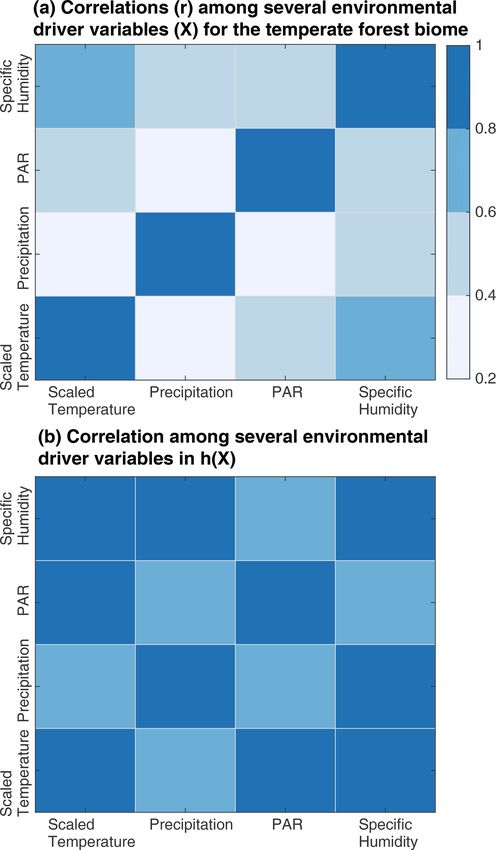
single coefficient or scaling factor (β) for this column. These Figure 2. Correlation coefficients (r) between environmental
fluxes are input into the regression at a 4◦ latitude by 5◦ drivers over temperate forests biome in year 2017 in X (a) and
longitude spatial resolution to match that of GEOS-Chem. h(X) (b). We find that the correlation between environmental
The Supplement Sect. S2 contains greater discussion of these drivers (X) are generally low (a), e.g., PAR and scaled tempera-
CO2 sources. ture, precipitation, and specific humidity; however, when these en-
vironmental drivers are passed through the transport model h() and
interpolated to the locations of OCO-2 observations, the correlation
2.7 Analysis using the TBMs between these drivers becomes much stronger (b), indicating high
collinearity.
We compare the estimated coefficients (β) from real OCO-2
observations against simulations using synthetic OCO-2 ob-
servations generated from 15 different TBMs in TRENDY We generate synthetic OCO-2 observations using each of
(v8). We list out all of the individual models in the TRENDY these TBM flux estimates. To do so, we first regrid each
comparison in Table S1. Model outputs from the TRENDY of the TRENDY model estimates to a spatial resolution of
project were provided at a monthly time resolution, and the 4◦ latitude by 5◦ longitude, the spatial resolution of the
spatial resolution varies from one model to another (though GEOS-Chem model. We then run the TRENDY model fluxes
many models have a native spatial resolution of either 0.5◦ through the GEOS-Chem model for years 2015–2018 and in-
latitude–longitude or 1◦ latitude–longitude). We specifically terpolate the model outputs to the times and locations of the
use TRENDY model outputs from scenario 3 simulations, in OCO-2 observations.
which all TBMs are forced with time-varying CO2 , climate,
and land use.
https://doi.org/10.5194/acp-21-6663-2021 Atmos. Chem. Phys., 21, 6663–6680, 20216670 Z. Chen et al.: Global CO2 fluxes from space
3 Results and discussion lenge in relating satellite-based CO2 observations to pat-
terns in environmental drivers. The environmental driver
3.1 Results of model selection datasets are passed through the GEOS-Chem model (h())
and interpolated the locations of OCO-2 observations as
The model selection results highlight the strengths and limi- part of the regression (h(X), Eqs. 1 and 3). In other words,
tations of using current OCO-2 observations to estimate rela- these driver datasets are input into GEOS-Chem in place of
tionships with environmental driver datasets. We use model a traditional CO2 flux estimate. This step is necessary so
selection based on the BIC to determine a set of environmen- that the environmental driver datasets can be directly com-
tal driver datasets to include in the analysis using OCO-2 pared against patterns in the OCO-2 observations. The driver
observations and using the TBMs. We only select 10 envi- datasets (i.e., columns of X) that we use in the regression
ronmental driver datasets when we run model selection on are generally unique from one another (i.e., have unique spa-
the OCO-2 observations – both when we use environmental tial and temporal patterns). However, the differences among
driver datasets from the CRUJRA and MERRA-2 products. many driver datasets disappear once those datasets have been
We are generally able to identify at least one or two key en- passed through GEOS-Chem. Figure 2 displays the corre-
vironmental relationships in each biome using total column lation coefficients (r) among environmental driver datasets
CO2 observations (shown on the x axis of Fig. 3). With that from MERRA-2 for temperate forests, both before (Fig. 2a)
said, we are only able to quantify relationships with these and after (Fig. 2b) those driver datasets have been passed
few, salient environmental variables. More detailed environ- through GEOS-Chem and interpolated to the OCO-2 obser-
mental relationships within each biome are difficult to dis- vations. The correlation coefficients increase substantially
cern. from the former to the latter case. This colinearity is inde-
Note that we select a similar number of environmental pendent of errors in the OCO-2 observations and indicates a
driver datasets when using synthetic OCO-2 observations hard limit on the number of relationships with environmen-
that are generated from each of the TBMs. We select any- tal driver datasets (i.e., coefficients) that we can quantify in
where between 8 and 13 environmental driver datasets (an the regression. In other words, model selection results are at
average of 10 datasets) in the analysis using each of the least partially limited by the limited sensitivity of OCO-2 ob-
TBMs. This result indicates consistency between the anal- servations to variations in these environmental driver datasets
ysis using real OCO-2 observations and the analysis using – either due to atmospheric smoothing and/or due to limita-
synthetic OCO-2 observations generated using CO2 fluxes tions in the availability of OCO-2 observations in some re-
from each of the 15 different TBMs. gions of the globe. This limitation is in addition to the un-
Overall, we have difficulty detecting the unique contribu- certainties due to errors in the OCO-2 observations and the
tions of many environmental driver datasets to variability in GEOS-Chem model, which also have a critical impact on in-
the OCO-2 observations. This issue is highlighted by an ex- ferences about CO2 fluxes using OCO-2 observations (e.g.,
amination of colinearity in the regression model. In a re- Chevallier et al., 2007, 2014; Miller et al., 2018).
gression, we cannot estimate different coefficients (β) for
two predictor variables (i.e., columns of X) that are iden- 3.2 Environmental relationships inferred using
tical or nearly identical; the regression cannot be used to observations from OCO-2
estimate unique coefficients because the predictor variables
themselves are not unique. In regression modeling, this phe- We are able to quantify the relationships between OCO-2
nomenon is known as colinearity. The coefficients (β) es- observations and several key environmental driver datasets.
timated for colinear variables are often unrealistic, and the Figures 3 and 4 display the estimated coefficients from the
standard errors or uncertainties in those coefficients (Vβ̂ ) are regression analysis using observations from OCO-2. Across
often unexpectedly large (e.g., Ramsey and Schafer, 2012). extratropical biomes, PAR is the most commonly selected
Model selection is one way to reduce or remove colinearity; variable. This result reflects the fact that light availability is
colinear variables, by definition, do not contribute unique in- a key factor that drives CO2 flux variability in mid-to-high
formation to a regression and are therefore rarely selected latitudes (e.g., Fang and Michalak, 2015; Baldocchi et al.,
using a model selection approach like the BIC. One common 2017). As expected, the estimated coefficients for PAR are
method for detecting colinearity is to estimate the correla- negative, indicating that an increase (or decrease) in PAR in
tion coefficient (r) between different columns of X; a value the model is associated with a decrease (or increase) in NEE
greater than ∼ 0.55 can indicate the presence of colinearity and an increase (or decrease) in carbon uptake. Note that in
(e.g., Ratner, 2012). this study negative values for NEE refer to CO2 uptake while
We find substantial colinearity in the regression analy- positive values refer to net CO2 release to the atmosphere.
sis (Fig. 2). This colinearity likely plays an important role By contrast, precipitation and scaled temperature are
in the model selection results, in addition to errors in the the most commonly selected environmental driver datasets
OCO-2 observations and errors in the GEOS-Chem model; across tropical biomes. The magnitude of the coefficients for
it represents an important but potentially overlooked chal- each of these two variables is similar in most biomes, indi-
Atmos. Chem. Phys., 21, 6663–6680, 2021 https://doi.org/10.5194/acp-21-6663-2021Z. Chen et al.: Global CO2 fluxes from space 6671
cating that patterns in both have similarly important associ-
ations with patterns in CO2 fluxes. Specifically, a negative
coefficient assigned to scaled temperature indicates that an
increase in air temperature is associated with increased car-
bon uptake when air temperatures are cool and reduced car-
bon uptake when air temperatures are hot; the scaled tem-
perature function has the shape of an upside-down parabola,
and temperature thus has a different association with CO2
fluxes depending upon whether the air temperature is above
or below the optimal temperature for photosynthesis (e.g.,
Fig. S1). Indeed, high temperatures in the tropics often ex-
ceed the optimal temperature for photosynthesis (e.g., Bal-
docchi et al., 2017), which reduces carbon uptake (e.g.,
Doughty and Goulden, 2008). Furthermore, negative coef-
ficients for precipitation indicate that an increase in precipi-
tation is associated with an increase in carbon uptake, which
is in line with current knowledge that water availability fa-
cilitates photosynthesis across seasonal to annual temporal
scales, especially in arid or semiarid regions (e.g., Gatti et al.,
2014; Jung et al., 2017).
In addition to this regression analysis, we use a GIM to
estimate the stochastic component of the fluxes (ζ , Eq. 1) –
patterns in the fluxes that are implied by the OCO-2 obser-
vations but do not match any existing environmental driver
dataset. To this end, Fig. 5 shows the mean contribution of
each environmental driver variable and the stochastic com-
ponent to the GIM across years 2015–2018 using MERRA-2
for the environmental driver datasets. The magnitude of the
stochastic component in this plot is small relative to the con-
tribution of different environmental variables and relative to
the contribution of anthropogenic sources. Furthermore, the
stochastic component contains very diffuse spatial patterns,
and these very broad patterns do not imply any clear defi-
ciency in the other components of the GIM. For example, the
regression component of the GIM (Xβ̂) accounts for 89.6 %
of the variance in the estimated fluxes, and the stochas-
tic component conversely accounts for only 10.4 % of the
flux variance. Furthermore, the regression component, when Figure 3. Estimated coefficients (β) from the TRENDY models
passed through the GEOS-Chem model, matches OCO-2 ob- (blue), from the ensemble mean of the TRENDY models (black),
servations nearly as well as the full posterior flux estimate and from the analysis using OCO-2 (red). Each blue or red dot in-
(Figs. S2 and S13). This result shows that a limited number dicates the mean value across all 4 years of the study period. Gray
of environmental driver datasets can adeptly reproduce broad bars indicate the full range of uncertainties in the coefficients. To
patterns in CO2 fluxes across continental and global spatial construct these gray bars, we calculate the uncertainties in the coef-
ficients estimated for each individual TBM (or for the real OCO-2
scales but reinforces the conclusion that current OCO-2 ob-
data) using Eq. (4). They gray bars encapsulate all of the uncertainty
servations are not sufficient to disentangle more complex en- bounds from all of these individual model calculations. Further-
vironmental relationships. more, the analysis of OCO-2 includes simulations using MERRA-
In all of the simulations using OCO-2 observations, we es- 2 meteorology with a simple formulation of 9 (red square), using
timate a scaling factor (β) for anthropogenic, biomass burn- CRUJRA meteorology and a simple formulation of 9 (red dot), and
ing, and ocean fluxes of near one, indicating that these source using MERRA-2 and a complex formulation of 9 (the same used
types have a magnitude that is broadly consistent with atmo- in the GIM, red triangle). The coefficients from the analysis using
spheric observations. Specifically, the estimated scaling fac- OCO-2 (red) are broadly within the range of the estimates in TBMs
tor estimated ranges from 0.97 to 1.05, depending upon the (blue). We further calculate the coefficient of variation (CV) of co-
year and simulation. Note, however, that we estimate a single efficients for each environmental driver within the TBMs (b), and
scaling factor for all of these source types combined and are we find that the largest CVs are from the coefficients for precipita-
tion.
unable to confidently constrain separate scaling factors for
https://doi.org/10.5194/acp-21-6663-2021 Atmos. Chem. Phys., 21, 6663–6680, 20216672 Z. Chen et al.: Global CO2 fluxes from space
Figure 4. This figure is similar to Fig. 3 but shows results for individual years. There are no noticeable shifts in the coefficient estimates
between El Niño (2015–2016; a–b) and non-El Niño years (2017–2018; c–d) from the analysis using OCO-2 (red). Some individual TBMs
show differences of up to 50 % in the estimated coefficient among years, though many individual TBMs do not.
each source, a topic discussed in greater detail in the Supple- 3.3 Comparison between inferences from OCO-2 and
ment Sect. S2. TBMs
Note that the inferences described here are also broadly
consistent with independent, ground-based atmospheric ob- The environmental relationships (i.e., coefficients) estimated
servations. We specifically model atmospheric CO2 using for the TBMs show a substantial range (Figs. 3 and 4); this
fluxes estimated from the GIM and compare against regular spread highlights uncertainties in state-of-the-art TBMs and
aircraft observations, campaign data from the Atmospheric indicates that there is an opportunity to help inform these re-
Tomography Mission (ATom; Wofsy et al., 2018), and obser- lationships using atmospheric CO2 observations. On the one
vations from the Total Carbon Column Observing Network hand, we are only able to infer a limited number of environ-
(TCCON; Wunch et al., 2011). In most instances, the model mental relationships using current observations from OCO-2,
result matches the observations to within the errors specified and this fact limits the extent to which we can inform TBM
in the inverse model (i.e., to within the errors specified in development using available space-based CO2 observations.
the R covariance matrix), and the model–data comparisons On the other hand, we can infer relationships with several
do not exhibit any obvious seasonal biases. Furthermore, we key environmental drivers (e.g., Fig. 3), and TBMs disagree
also model XCO2 using the outputs of the regression analy- on relationships with even these key drivers. This result thus
sis (Xβ̂), and these outputs also show good agreement with indicates the limitations of this analysis but also its strengths.
OCO-2 observations (Fig. S13). The Supplement Sect. S4, Specifically, Figs. 3 and 4 graphically display these results
Figs. S2–S13, and Tables S2–S3 describe these comparisons from the regression analysis – the coefficients estimated us-
in greater detail. ing OCO-2 observations compared to those estimated from
the TRENDY models. The coefficients from the OCO-2 anal-
ysis are almost always within the range of those estimated
using the ensemble of TBMs. With that said, the coefficients
estimated for many of the TBMs are far from the value esti-
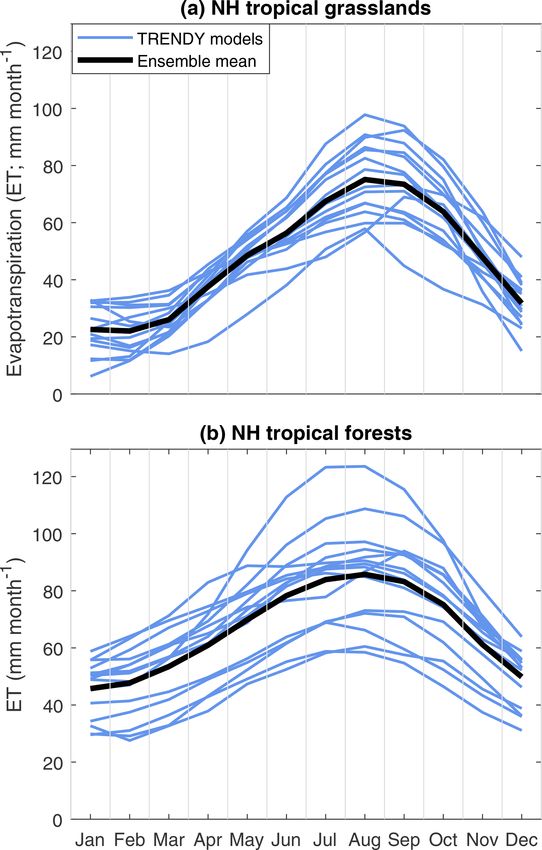
Atmos. Chem. Phys., 21, 6663–6680, 2021 https://doi.org/10.5194/acp-21-6663-2021Z. Chen et al.: Global CO2 fluxes from space 6673 Figure 5. The contribution of different environmental driver datasets to the flux estimate from the GIM. Panel (a) displays the 4-year mean flux estimate (including both the regression and stochastic components of the flux estimate; units of µmol m−2 s−1 ) and panel (b) the contribution from anthropogenic, biomass burning, and ocean fluxes. Contributions from different environmental drivers, including scaled temperature (c), precipitation (d), and PAR (e), describe most of spatiotemporal variability in terrestrial biospheric CO2 fluxes, whereas the stochastic components (ζ ) (f) only account for a small portion of flux variability. Note that the inverse modeling results shown in this figure use environmental driver data from MERRA-2. Also note that the color bars used in panels (a)–(b), (c)–(e), and (f) are different. White colors in panels (c)–(e) indicate that not all environmental drivers are selected in all biomes. mated using OCO-2, implying that observations from OCO- efficient from the ensemble of TBMs. In addition, the TBMs 2 can be used to inform the relationships within numerous are evenly split on whether the relationship with precipitation individual models. Note that in Figs. 3 and 4 the x axis is is positive or negative across tropical biomes, and our anal- ordered based upon the environmental driver variables that ysis using OCO-2 observations agrees with models that esti- are selected using OCO-2, and we show the estimated coef- mate a negative relationship (i.e., precipitation is associated ficients for TBMs in which the listed environmental driver with greater CO2 uptake). There is substantial disagreement variable is also chosen using model selection. Furthermore, on the magnitude of this relationship, even among models the coefficients shown for the TBMs in Figs. 3 and 4 are cal- that yield a negative relationship; the estimate using OCO-2 culated using environmental driver datasets from CRUJRA. observations falls in the midrange of these TBMs for both Figure S14 displays the results for the TBMs using environ- tropical biomes. mental driver data from MERRA-2, and the results look sim- More broadly, the TBMs simulate very different water cy- ilar to those using CRUJRA. cling through each ecosystem, in spite of the fact that each We specifically find large differences between the analysis model uses the same precipitation inputs from CRUJRA. using OCO-2 and the TBMs for relationships with precipi- These broader differences in water cycling within the TBMs tation. The relationships between precipitation are arguably may help explain the large uncertainties in the relationships more uncertain within the TBMs than the relationships with between CO2 and precipitation and highlight an important other environmental variables (Fig. 3a) and are more uncer- source of uncertainty within these models. Specifically, we tain in tropical biomes than temperate ones. This statement find that estimated evapotranspiration (ET) across the TBMs is particularly apparent when we examine the coefficient of differs by almost a factor of 3 among models in some seasons variation for each relationship (Fig. 3b). The coefficient of and biomes, and annual ET ranges from 375 to 700 mm over variation is a measure of the uncertainty relative to the mag- northern hemispheric tropical grasslands (Fig. 6a) and from nitude of the mean, and Fig. 3b shows the standard deviation 530 to 1010 mm over northern hemispheric tropical forests in the coefficients from the 15 TBMs divided by the mean co- (Fig. 6b). These large differences in ET estimates reinforce https://doi.org/10.5194/acp-21-6663-2021 Atmos. Chem. Phys., 21, 6663–6680, 2021
6674                                                                               Z. Chen et al.: Global CO2 fluxes from space

                                                                      timescales considered (e.g., Baldocchi et al., 2017). For ex-
                                                                      ample, excess precipitation is associated with limited light
                                                                      availability in regions like the humid tropics and can raise
                                                                      the water table to a level that inhibits respiration. With that
                                                                      said, short-term rain events have been shown to boost respi-
                                                                      ration (e.g., Baldocchi, 2008).
                                                                         Like precipitation, relationships with PAR are also highly
                                                                      uncertain in the simulations using TBMs. Most models yield
                                                                      relationships with the same sign, but those relationships vary
                                                                      widely in magnitude. By contrast, results using OCO-2 ob-
                                                                      servations are very similar to the ensemble mean of the
                                                                      TBMs. This result is particularly interesting given that the
                                                                      individual TBMs do not show consensus with one another.
                                                                      The differences among the TBMs likely stem from the fact
                                                                      that these TBMs exhibit widely varying seasonal cycles and
                                                                      peak growing season uptake across extratropical biomes. For
                                                                      example, in temperate forests (e.g., Fig. S17), the maximum
                                                                      monthly carbon uptake differs by a factor of 8 among the
                                                                      TBMs, and a handful of TBMs estimate a very different sea-
                                                                      sonal cycle than the bulk of the TBMs with maximum uptake
                                                                      during the middle of the growing season.
                                                                         In contrast to the discussion of precipitation and PAR, ex-
                                                                      isting TBMs yield much better agreement on the relation-
                                                                      ships between CO2 and scaled temperature (Fig. 3). In tropi-
                                                                      cal biomes, nearly all TBMs agree on the sign of the relation-
                                                                      ship, and the estimates using OCO-2 observations are within
                                                                      the range of those estimated using TBMs. Interestingly, the
                                                                      uncertainty bounds on the coefficient estimate using OCO-2
                                                                      are not that much smaller than the range of coefficients from
Figure 6. Four-year-averaged evapotranspiration (ET) estimates        the ensemble of TBMs, both for tropical grasslands and es-
from a suite of 15 TBMs (blue) and from the ensemble mean (black)     pecially for tropical forests. This result points to relatively
for northern hemispheric tropical grasslands (a) and for northern     good consensus in modeled relationships with temperature
hemispheric tropical forests (b). Annual ETs show large differences
                                                                      for tropical grasslands and forests – both using TBMs and
in magnitude across the TBMs for both tropical biomes.
                                                                      OCO-2 observations. However, it also indicates that atmo-
                                                                      spheric observations from OCO-2 potentially have less op-
                                                                      portunity to inform these relationships than for precipitation
the very different responses of tropical ecosystems in these          or PAR where TBMs do not show consensus.
models (both tropical forests and tropical grasslands) to pre-           The comparisons described above are largely from biomes
cipitation inputs.                                                    centered in the tropics and midlatitudes and include few com-
   Indeed, existing studies have indicated large uncertainties        parisons for high-latitude biomes (e.g., the boreal forest or
in the responses of tropical forests to water availability (e.g.,     tundra biomes). For example, we do not select any environ-
Restrepo-Coupe et al., 2016) and have offered several possi-          mental driver variables for the tundra biome using OCO-2
ble explanations. Soil depths and rooting distribution are par-       and only select PAR in boreal forests. OCO-2 observations
ticularly challenging to model in tropical ecosystems, yield-         are sparse across high latitudes both due to the lack of sun-
ing uncertainties in the relationship between water availabil-        light in winter and due to frequent cloud cover in many high-
ity and CO2 fluxes (e.g., Baker et al., 2008; Poulter et al.,         latitude regions. We also only select PAR in boreal forests in
2009). For example, Poulter et al. (2009) argued that current         simulations using 2 of the 15 TBMs. This result also reflects
TBMs tend to underestimate soil depths in tropical forests,           the limited availability of OCO-2 observations over high-
which are critical to guarantee soil water access and to ac-          latitude regions; for the analysis here, we create synthetic
curately simulate dry-season photosynthesis in TBMs. The              OCO-2 observations using each TBM and apply model se-
treatment of irrigation and other land management practices           lection to each of these synthetic OCO-2 datasets. Hence, the
also differs among models and creates further uncertainty             sparsity of OCO-2 observations not only affects the model
(e.g., Le Quéré et al., 2018; Pan et al., 2020). To compli-           selection results using real OCO-2 observations but also af-
cate matters, the role of precipitation in carbon dynamics can        fects the analysis shown in Figs. 3 and 4 using the TBMs.
vary depending on broader environmental conditions and the            The fact that PAR is selected for so few TBMs is not a reflec-

Atmos. Chem. Phys., 21, 6663–6680, 2021                                                https://doi.org/10.5194/acp-21-6663-2021
Z. Chen et al.: Global CO2 fluxes from space 6675
tion on the important role of PAR across the boreal forest in order to reduce these uncertainties, scientists will likely need
many TBMs. to reconcile differences in the environmental processes that
Note that the analysis described above is based upon the drive these CO2 flux estimates. Existing studies have used
mean relationships that we infer for years 2015–2018. We in situ atmospheric observations to help quantify and evalu-
also explored how these relationships in the models vary ate these relationships across the extratropics (e.g., Fang and
during El Niño (2015–2016) and non-El Niño years (2017– Michalak, 2015; Hu et al., 2019). However, this task is much
2018) (Fig. 4). The relationships that we estimate do not fun- more challenging across regions of the globe with sparse in
damentally change between El Niño and non-El Niño years situ observations, including most of the tropics. In spite of
and neither does the spread among the models. This result in- the limitations described in this study, the advent of satellite-
dicates two conclusions: (1) there is not a fundamental shift based CO2 observations like those from OCO-2 provides a
in these relationships between El Niño versus non-El Niño new opportunity to constrain these environmental relation-
years, suggesting that it is not the change in environmen- ships and thereby provide unique atmospheric constraints on
tal relationships but the change in environmental variables the global carbon cycle.
themselves that correlates with the change in flux estimates;
and (2) the uncertainties in the relationships, as estimated
by the TBMs, are not higher in El Niño versus non-El Niño Data availability. The version 9 of 10 s average OCO-2 retrievals is
years. With that said, the magnitude of the estimated coeffi- available at ftp://ftp.cira.colostate.edu/ftp/BAKER/ (last access: 29
cient does change in some models between El Niño and non- October 2020, Baker, 2019); data information of the OCO-2 MIP
El Niño years; the changes in the coefficients are generally is available at https://www.esrl.noaa.gov/gmd/ccgg/OCO2/ (last ac-
cess: 9 November 2020, OCO-2 MIP team, 2020); data information
less than 50 % in most models, and the models do not show
of the ObsPack data product is available at http://www.esrl.noaa.
a consistent direction of change between El Niño and non-El
gov/gmd/ccgg/obspack/ (last access: 20 September 2020, Coopera-
Niño years. tive Global Atmospheric Data Integration Project, 2019).
4 Conclusions Supplement. The supplement related to this article is available on-
line at: https://doi.org/10.5194/acp-21-6663-2021-supplement.
In this study, we use 4 years of observations from OCO-2
and a top-down statistical framework to evaluate the rela-
tionships between patterns in atmospheric CO2 observations Author contributions. ZC and SMM designed the study, analyzed
and patterns in environmental driver datasets that are com- the data, and wrote the manuscript. SS, PF, VB, DSG, VH, AJ, EJ,
monly used in modeling the global carbon cycle. We are able EK, SL, DLL, PCM, JRM, JEMSN, BP, HT, AJW, and SZ provided
to quantify a limited number of these environmental relation- TRENDY model flux estimates. All authors reviewed and edited the
ships using observations from OCO-2. In spite of these limi- paper.
tations, we are still able to identify relationships with a small
number of salient environmental driver datasets, and state-
of-the-art TBMs do not show consensus on some of these Competing interests. The authors declare that they have no conflict
of interest.
key relationships, indicating an opportunity to inform these
relationships using atmospheric CO2 observations.
We subsequently compare inferences using OCO-2 against
Acknowledgements. We thank Kim Mueller and Anna Michalak
inferences from 15 state-of-the-art TBMs that have model for their feedback on the research; David Baker for his help with
outputs available for the same set of years. For the broad the XCO2 data; Colm Sweeny and Kathryn McKain for their help
regions and time span explored in this study, we find neg- with aircraft datasets from the NOAA/ESRL Global Greenhouse
ative relationships between patterns in OCO-2 observations Gas Reference Network; John Miller, Luciana Gatti, Wouter Pe-
and patterns in precipitation; this result agrees with half of ters, and Manuel Gloor for their help with the aircraft data from
the TBMs, which do not show consensus on relationships the INPE ObsPack data product; Steven Wofsy, Kathryn McKain,
with precipitation. By contrast, TBMs exhibit much greater Colm Sweeny, and Róisín Commane for their help with ATom air-
skill in describing relationships with scaled temperature, as craft datasets; and Debra Wunch for her help with the TCCON
implied by the relatively good agreement among TBMs. In datasets. Daven Henze’s work is supported by NOAA grant no.
fact, the uncertainties in the temperature relationship across NA16OAR4310113. Daniel Goll’s work is supported by the ANR
CLAND Convergence Institute. The data analysis and inverse mod-
tropical biomes, as estimated using OCO-2 observations, are
eling were performed on the NASA Pleiades Supercomputer.
nearly as large as the range of estimates using TBMs.
More broadly, state-of-the-art TBMs disagree on the con-
tribution of individual biomes to the global carbon balance, a Financial support. This research has been supported by NASA
result highlighted in several studies (e.g., Poulter et al., 2014; ROSES (grant no. 80NSSC18K0976).
Sitch et al., 2015; Ahlström et al., 2015; Piao et al., 2020). In
https://doi.org/10.5194/acp-21-6663-2021 Atmos. Chem. Phys., 21, 6663–6680, 2021You can also read