A satellite-data-driven framework to rapidly quantify air-basin-scale NOx emissions and its application to the Po Valley during the COVID-19 pandemic
←
→
Page content transcription
If your browser does not render page correctly, please read the page content below
Atmos. Chem. Phys., 21, 13311–13332, 2021
https://doi.org/10.5194/acp-21-13311-2021
© Author(s) 2021. This work is distributed under
the Creative Commons Attribution 4.0 License.

A satellite-data-driven framework to rapidly quantify
air-basin-scale NOx emissions and its application to the
Po Valley during the COVID-19 pandemic
Kang Sun1,2 , Lingbo Li1 , Shruti Jagini1 , and Dan Li3
1 Department of Civil, Structural and Environmental Engineering, University at Buffalo, Buffalo, NY, USA
2 Researchand Education in Energy, Environment and Water Institute, University at Buffalo, Buffalo, NY, USA
3 Department of Earth and Environment, Boston University, Boston, MA, USA

Correspondence: Kang Sun (kangsun@buffalo.edu)

Received: 26 March 2021 – Discussion started: 25 May 2021
Revised: 22 July 2021 – Accepted: 10 August 2021 – Published: 8 September 2021

Abstract. The evolving nature of the COVID-19 pandemic             The tropospheric VCD (TVCD) retrieval of NO2 has been
necessitates timely estimates of the resultant perturbations       widely used to infer the emissions of nitrogen oxides
to anthropogenic emissions. Here we present a novel frame-         (NOx = NO2 + NO), which is at the center stage of at-
work based on the relationships between observed column            mospheric chemistry by modulating ozone and secondary
abundance and wind speed to rapidly estimate the air-basin-        aerosol formation (Kroll et al., 2020). The NOx emissions are
scale NOx emission rate and apply it at the Po Valley in Italy     dominated by anthropogenic fossil fuel combustion, and its
using OMI and TROPOMI NO2 tropospheric column obser-               chemical lifetime in the lower troposphere is relatively short.
vations. The NOx chemical lifetime is retrieved together with      Consequently, the satellite-observed NO2 TVCD is highly
the emission rate and found to be 15–20 h in winter and 5–         responsive to perturbations of human activities, including
6 h in summer. A statistical model is trained using the esti-      economic recession (Castellanos and Boersma, 2012; Russell
mated emission rates before the pandemic to predict the tra-       et al., 2012), long- and short-term emission regulations (Dun-
jectory without COVID-19. Compared with this business-as-          can et al., 2016; Mijling et al., 2009; Witte et al., 2009), and
usual trajectory, the real emission rates show three distinctive   the ongoing global pandemic caused by the coronavirus, or
drops in March 2020 (−42 %), November 2020 (−38 %), and            COVID-19 (Bauwens et al., 2020; Liu et al., 2020; Huang
March 2021 (−39 %) that correspond to tightened COVID-             and Sun, 2020).
19 control measures. The temporal variation of pandemic-              Although NO2 TVCD is well established as an indica-
induced NOx emission changes qualitatively agrees with             tor of NOx emission, the quantitative connection between
Google and Apple mobility indicators. The overall net NOx          NO2 abundance and NOx emission is confounded by non-
emission reduction in 2020 due to the COVID-19 pandemic            linear chemistry and meteorology (Valin et al., 2014; Gold-
is estimated to be 22 %.                                           berg et al., 2020; Keller et al., 2021). Many NOx emis-
                                                                   sion inference methods have been proposed using chemical
                                                                   transport models (CTMs) that resolve chemistry and mete-
                                                                   orology in space and time, including mass balance (Martin
1   Introduction                                                   et al., 2003; Lamsal et al., 2011; Zheng et al., 2020), four-
                                                                   dimensional variational data assimilation (4D-Var, Qu et al.,
Satellites have revolutionized our ability to observe the          2019; Wang et al., 2020), and Kalman filters (Miyazaki et al.,
Earth’s atmospheric composition and air quality. Verti-            2020a; Mijling and Van Der A, 2012; Ding et al., 2020). Ding
cal column densities (VCDs) of reactive species such as            et al. (2020) and Miyazaki et al. (2020b) used CTMs to es-
NO2 , HCHO, SO2 , and NH3 are retrieved from the ob-               timate NOx emission reduction in China in the early phase
served radiances in the ultraviolet, visible, or infrared bands.

Published by Copernicus Publications on behalf of the European Geosciences Union.
13312 K. Sun et al.: Observational-data-driven emission and lifetime estimates over air basins
of the COVID-19 pandemic, but it is a growing challenge to stantial increase in retrieved NO2 TVCD in polluted regions.
match the resolution, lag time, and running cost of CTMs The TROPOMI NO2 algorithm is expected to be updated
with the new generation of satellite products that resolve the with full reprocessing in 2021 to improve its consistency and
NO2 spatial distribution down to a few kilometers. As such, continuity (GES DISC, 2021). The level 2 orbits covering the
observational-data-driven approaches have also been devel- geographical region of interest over every month are stan-
oped, which attempt to derive emissions based on the ob- dardized into single files from October 2004 to June 2021
served column abundance and without invoking CTMs. A for OMI and from May 2018 to June 2021 for TROPOMI.
common way to estimate emissions of short-lived species We only use quality-assured level 2 pixels with cloud frac-
like NOx is to retrieve emission and lifetime simultaneously tion < 0.3 and solar zenith angle < 70◦ . Throughout the OMI
by fitting an exponentially modified Gaussian (EMG) func- mission, its across-track pixels are limited to 5–23 out of 1–
tion to the downwind plumes from relatively isolated emis- 60 to avoid the row anomaly and keep the time series analy-
sion sources (e.g., cities or power plants) (Beirle et al., 2011; sis consistent (Duncan et al., 2016; Schenkeveld et al., 2017).
Liu et al., 2016; de Foy et al., 2015; Lu et al., 2015; Gold- TROPOMI features 450 pixels across its 2600 km swath and
berg et al., 2019a, b; Laughner and Cohen, 2019; Valin et al., a nadir pixel size of 3.5 × 5.5 km2 (3.5 × 7 km2 before 6 Au-
2013; Zhang et al., 2019). However, the observational-data- gust 2019), leading to significantly higher spatial resolution
driven approaches using OMI only provide warm-season than OMI, whose nadir pixel size is 13 × 24 km2 .
or annually averaged emissions and hence cannot capture Validation studies of both OMI and TROPOMI NO2
the rapidly varying and ongoing COVID-19-induced emis- TVCDs consistently show systematic low biases (Choi et al.,
sion changes. The availability of much more finely resolved 2020; Judd et al., 2020; Verhoelst et al., 2021), which can be
TROPOMI observations since 2018 enables observation- attributed to the horizontally coarse a priori profile represen-
based NOx emission estimates at daily scale over a megac- tation as well as uncertainties in surface albedo and cloud pa-
ity (Lorente et al., 2019). rameters in the air mass factor (AMF) calculation. This low
Based on satellite observations and reanalysis wind speed, bias matters less for emission trend analysis but will propor-
we develop a novel framework that directly and quickly tionally impact the absolute values of the derived emission
quantifies air-basin-scale NOx emissions at monthly reso- rate. This study focuses on an air basin in which a high level
lution. We demonstrate this framework using NO2 TVCDs of pollution is confined, and the spatial gradient is signifi-
from both OMI and TROPOMI over the Po Valley air basin cantly less than many other polluted regions. The relative bi-
in Italy, which has been severely affected by COVID-19 (Fil- ases between OMI and TROPOMI NO2 TVCD are assessed
ippini et al., 2020). The COVID-19-induced emission decline by comparing strictly collocated level 2 retrievals and given
has to be disentangled from pre-existing trends and season- in Appendix A. The OMI NO2 TVCD is generally higher
ality. Leveraging the long data record from OMI, we build than TROPOMI in the cold season, with a monthly OMI–
a statistical model using historic emission rates and predict TROPOMI normalized mean bias (NMB) up to over 30 %,
the business-as-usual trajectory in 2020–2021. The differ- whereas the TROPOMI TVCD is generally higher in the
ence between this trajectory and the real 2020–2021 emis- warm season, with a monthly OMI–TROPOMI NMB down
sions reflects the net effect of COVID-19. As the pandemic to −20 %.
and the controlling policies are still evolving in 2021, this
extrapolation using a long-term satellite record offers a sig- 2.2 Study domain and NOx emission inventories
nificant advantage over a simple 2020 vs. 2019 comparison.
Although only NOx emission in the Po Valley is investigated The Po Valley air basin is delineated according to the bound-
in this work, this satellite-data-driven framework can be read- ary between the flat terrain in northern Italy and mountain
ily applied to other satellite products and regions to rapidly ranges in the north, west, and south as well as the Adri-
characterize emission changes. atic Sea coastline in the east, as shown in Fig. 1. The air
basin area is 6.6 × 10⁴ km2 . The west–east length scale is
∼ 500 km, and the south–north length scale is ∼ 300 km;
2 Materials both are larger than the square root of basin area (257 km)
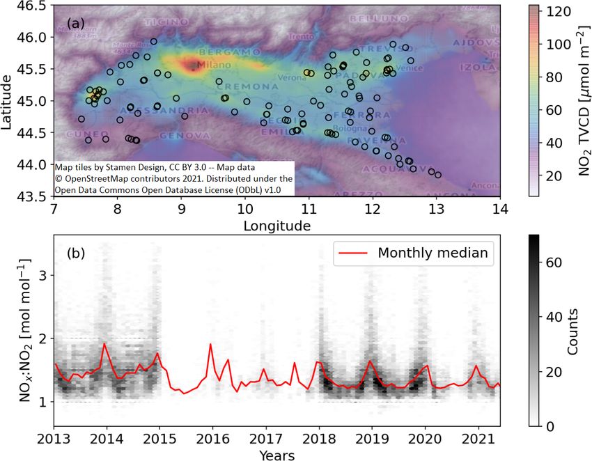
due to the irregularity of the basin shape. We contrast our de-
2.1 Satellite TVCDs rived monthly air-basin-scale NOx emission rates with four
global inventories. Their emission distributions near the Po
We use the most recent (version 4) NO2 level 2 TVCD re- Valley air basin are illustrated in Fig. 1. The Jet Propulsion
trievals from the NASA operational standard product for Laboratory (JPL) chemical reanalysis provides monthly top-
OMI (Lamsal et al., 2021). The operational TROPOMI NO2 down emission estimates at 1.1◦ × 1.1◦ spatial resolution for
product (van Geffen et al., 2020; ESA, 2018) used in this 2005–2019 (Miyazaki et al., 2019, 2020a). The NOx emis-
study underwent several algorithm updates since its public sions from the JPL chemical reanalysis (Fig. 1a) are con-
release in 30 April 2018. A significant cloud retrieval algo- strained by assimilating O3 , NO2 , CO, HNO3 , and SO2 from
rithm update happened in November 2020, leading to sub- the OMI, GOME-2, SCIAMACHY, MLS, TES, and MO-
Atmos. Chem. Phys., 21, 13311–13332, 2021 https://doi.org/10.5194/acp-21-13311-2021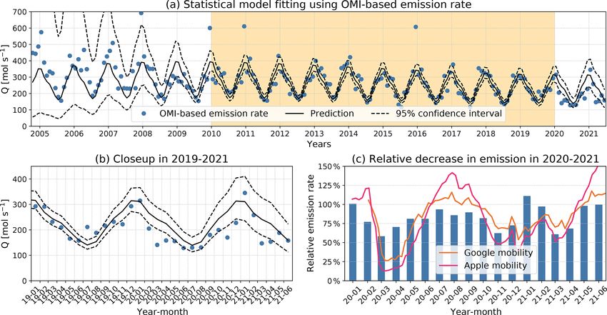
K. Sun et al.: Observational-data-driven emission and lifetime estimates over air basins                                     13313

PITT satellite instruments (Miyazaki et al., 2020a) and are      NOx available are included in the analysis. We include only
considered to have the highest accuracy in spite of the rel-     ground-based observations within OMI level 2 pixels with
atively low spatial resolution. The other three are bottom-      cloud fraction < 0.3, but the resultant all-sky vs. clear-sky
up emission inventories, including the Community Emission        differences are insignificant.
Data System (CEDS; McDuffie et al., 2020), the Emis-
sions Database for Global Atmospheric Research version
4.3.2 (EDGAR; Crippa et al., 2018), and the Peking Uni-          3     Methods
versity NOx inventory (PKUNOx; Huang et al., 2017). The
CEDS inventory is spatially resolved at 0.5◦ × 0.5◦ (Fig. 1b)    3.1    Construction of column–wind speed relationships
and available monthly from 1970 to 2017. Both EDGAR                     by physical oversampling
and PKUNOx are at 0.1◦ × 0.1◦ spatial resolution (Fig. 1c,
d). EDGAR is available annually from 1970 to 2012, and           A key step to estimating NOx emissions from the observed
PKUNOx is available monthly from 1960 to 2014. Because           NO2 TVCDs is to construct the column–wind speed rela-
of the large grid sizes of the JPL chemical reanalysis and       tionship by averaging column amounts over a range of wind
CEDS inventory, we calculate the air-basin-mean emission         speed intervals. Physical oversampling (Sun et al., 2018) pro-
rate by averaging inventory grid cells that overlap with the     vides a flexible way to spatiotemporally average satellite data
Po Valley air basin, weighted by the overlapping area.           with proper weighting and slice the data under different envi-
                                                                 ronmental conditions (e.g., wind speed). The averaged NO2
2.3   Wind fields                                                TVCD (hi) given sets of filtering criteria with respect to
                                                                 space (s), time (t), and other level 2 parameters (p) can be
We use wind fields gridded at 0.25◦ × 0.25◦ spatial reso-        calculated as
lution and hourly temporal resolution from the ERA5 re-                          P P
analysis meteorology (Hersbach et al., 2020). The relevant                         j ∈s   i∈t,p wi, j i
ERA5 fields are spatiotemporally interpolated at each indi-      hi(s, t, p) = P P                      .                   (1)
                                                                                     j ∈s   i∈t,p wi, j
vidual OMI and TROPOMI level 2 observation. Previous
observational-data-driven emission inference studies repre-      Here j is the index of each level 3 grid cell at 0.01◦ reso-
sented horizontal advection of NO2 (or similar short-lived       lution, and j ∈ s includes all grid cells satisfying the spatial
tracers like SO2 and NH3 ) by 10 m wind above the sur-           aggregation criterion s (e.g., within the boundary of an air
face (de Foy et al., 2015), 100 m above the surface (Gold-       basin). i is NO2 TVCD retrieved at level 2 pixel i. i ∈ t
berg et al., 2020), vertically averaged wind from the sur-       and p keep only level 2 pixels satisfying time filtering cri-
face to 500 m (Lu et al., 2015; Liu et al., 2016; Gold-          teria (e.g., within a calendar month) and parameter filtering
berg et al., 2019a), or vertically averaged wind from the        criteria (e.g., wind speed at the level 2 pixel within a certain
surface to 1000 m (Fioletov et al., 2017; Dammers et al.,        interval). wi, j is the weight of level 2 pixel i at level 3 grid
2019). Figure 2 quantitatively compares the wind speeds of       cell j and depends on the spatial response of pixel i at grid
these four options using ERA5 data sampled at OMI level          cell j as well as the retrieval uncertainty at pixel i (Zhu et al.,
2 observations within the Po Valley air basin boundary (see      2017; Sun et al., 2018).
Fig. 1) from October 2004 to February 2021. These four              The column–wind speed relationship for an air basin over
wind speeds show strong linear correlation, with stronger        a certain time interval is an array of averaged NO2 TVCDs
winds when higher altitudes are involved. The surface–           over different wind speed intervals (every 0.5 m s−1 in this
1000 m wind speed is almost twice as strong as the 10 m          study):
wind, whereas the two intermediate options, the 100 m wind
and the surface–500 m wind, are similar with a difference of
                                                                 hi = [hi(0 m s−1 ≤ W < 0.5 m s−1 ), hi(0.5 m s−1
13 %. The wind directions among those four options show
much larger discrepancy, but only the wind speeds will be            ≤ W < 1.0 m s−1 ), . . . ],                                (2)
used in this study.
                                                                 where W is the horizontal wind speed that is interpolated at
2.4   In situ NOx observations                                   level 2 pixels and is representative of horizontal advection.
                                                                 The four wind speed options shown in Fig. 2 are tested in
We use the ground-based NOx observations over the Po Val-        this study. Figure 3 shows the column–wind speed (100 m
ley available from the air quality data portal of the European   wind here) relationships for OMI and TROPOMI over the Po
Environment Agency (EEA) to constrain the temporal varia-        Valley in December 2018–November 2020 grouped into four
tion of the NOx : NO2 ratio (EEA, 2021). The validated data      seasons. TROPOMI provides 2–3 times more coverage than
(E1a) are used for the years 2013–2019 and combined with         OMI, as indicated by the dot sizes, but ∼ 50 times more valid
up-to-date data (E2a) for 2020–2021. Only valid hourly data      level 2 pixels due to much finer spatial resolution, as labeled
labeled at 13:00 and 14:00 local time with both NO2 and          in the legends.

https://doi.org/10.5194/acp-21-13311-2021                                        Atmos. Chem. Phys., 21, 13311–13332, 2021
13314                              K. Sun et al.: Observational-data-driven emission and lifetime estimates over air basins

Figure 1. Spatial distribution of annual NOx emissions in 2005 near the Po Valley air basin (black dashed line) from (a) JPL chemical
reanalysis, (b) CEDS, (c) EDGAR, and (d) PKUNOx.

Figure 2. Correlations between speeds of 100 m wind and 10 m wind (a), 100 m wind and surface–500 m wind (b), 100 m wind and surface–
1000 m wind (c), 10 m wind and surface–500 m wind (d), 10 m wind and surface–1000 m wind (e), and surface–500 m wind and surface–
1000 m wind (f). Wind data are from ERA5 meteorology sampled at valid OMI NO2 observation locations in the Po Valley air basin in
2004–2021. The slopes labeled in the plot are from orthogonal regression, and r is the correlation coefficient (wind speed unit: m s−1 ).

Atmos. Chem. Phys., 21, 13311–13332, 2021                                               https://doi.org/10.5194/acp-21-13311-2021
K. Sun et al.: Observational-data-driven emission and lifetime estimates over air basins 13315
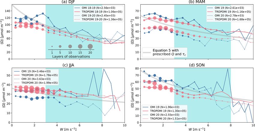
Figure 3. Relationships between OMI (blue) and TROPOMI (red) NO2 TVCDs and wind speeds in December, January, February (DJF, a),
March, April, May (MAM, b), June, July, August (JJA, c), September, October, and November (SON, d). Data are shown as solid lines for
2019 (including December 2018) and dotted lines for 2020 (including December 2019). Layers of level 2 observation coverage are indicated
by dot sizes. N in the legends denotes the total number of level 2 pixels used in each column–wind speed relationship. Thick gray lines show
the behaviors of Eq. (5) using prescribed NOx emission rates (Q) of 240, 170, 160, and 170 µmol m−2 and chemical lifetimes (τc ) of 16, 9,
5.5, and 11 h for the four seasons. A modest wind range of 3–8 m s−1 is highlighted by cyan shading.
3.2 Conceptual model of column–wind speed horizontal length scale of the air basin L:
relationships
L
τd = . (4)
The emission rate over an air basin Q can be linked to the W
basin-average column amount through a box model: This implicitly assumes that the horizontal wind efficiently
Q ventilates pollution away from the air basin. However, the
hi = , (3) Po Valley is surrounded by mountains except the east side.
1
φA τd + τ1c Low wind conditions may only circulate air pollution within
the basin boundary. We thus limit our analysis over moderate
where boldface symbols indicate vectors. The averaged NO2 wind speeds as shown in Fig. 3. We do not find systematic
TVCD hi and dynamic lifetime τ d are both vectors re- differences in column–wind relationships over different wind
solved over a range of wind speeds W , φ is the NOx : NO2 directions over moderate wind speeds, so all wind directions
ratio, A is the air basin area, and τc is the NOx chemical are combined to maximize the number of observations. Then,
lifetime. For cloud-free midday conditions in a polluted air the conceptual model of column–wind speed relationship can
mass, φ is conventionally assumed to be a constant of 1.32 be written as
with 20 % uncertainty in satellite-based NOx emission esti-
mates (Seinfeld and Pandis, 2006; Liu et al., 2016; Beirle Q
hi = . (5)
W
et al., 2019). We further constrain the temporal variation of φA L + τ1c
φ using observations in Sect. 4.3. The NOx chemical life-
time may vary with wind speed depending on complicated Van Damme et al. (2018) and de Foy et al. (2015) have ap-
nonlinear chemistry (Valin et al., 2013), so the scalar τc here plied such box models to estimate short-lived NH3 and NOx
should be considered the average value over the wind speed emission rates by prescribing their chemical lifetimes. The
range. The high noise level in column–wind speed relation- dynamic lifetime was neglected (Van Damme et al., 2018)
ships prevents us from obtaining further wind speed depen- or calculated as the ratio between the near-surface wind
dence of the chemical lifetime. We simplify the dynamic life- speed and the half-edge length of the square box (de Foy
time dimensionally as the ratio between wind speed and the et al., 2015). Similar box models have also been used to
https://doi.org/10.5194/acp-21-13311-2021 Atmos. Chem. Phys., 21, 13311–13332, 2021
13316                             K. Sun et al.: Observational-data-driven emission and lifetime estimates over air basins

infer area-integrated CH4 emission rates from column ob-          and τc are strongly anticorrelated, the error in τc is efficiently
servations (Buchwitz et al., 2017; Varon et al., 2018). The       propagated to the fitted Q. For example, the spikes in the ob-
chemical lifetime of CH4 is negligible, and the dynamic life-     served OMI column–wind speed relationships in Fig. 3c and
time was constrained by CTM simulations in these studies.         d would result in an unphysically low chemical lifetime and
Considering that the four wind options described in Sect. 2.3     unrealistically high emission rate without proper regulariza-
(10 m, 100 m, surface–500 m, and surface–1000 m) give dif-        tion. To reliably retrieve Q for each calendar month through-
ferent yet strongly correlated wind speed values (Fig. 2), we     out the OMI and TROPOMI record, we build a monthly cli-
expect that different L values are needed for those wind op-      matology of τc from aggregated observation data and use it
tions. End-to-end emission rate estimates are performed us-       as prior information in a Bayesian optimal estimation frame-
ing those four wind speed options with a range of L values in     work (Rodgers, 2000; Brasseur and Jacob, 2017). The steps
Sect. 4.1. We found that using 100 m wind√ and L = 280 km         are summarized below, followed by a description in this sec-
for the Po Valley air basin (close to A = 257 km) gives           tion.
emission rate estimates that are most consistent with the
JPL chemical reanalysis, which is considered to contain the         1. The monthly column–wind speed relationships are
smallest bias due to the high level of observational con-              aggregated into 12 months for all the years (“cli-
straints. This is deemed a calibration for the dynamic lifetime        matological months” hereafter, in contrast to calen-
and is specific to the Po Valley air basin.                            dar months) separately for OMI (2004–2021) and
   The behavior of Eq. (5) is shown in Fig. 3 as gray lines            TROPOMI (2018–2021). τc and Q are then fitted from
with prescribed emission rate Q and chemical lifetime τc               the column–wind speed relationship of each climatolog-
values for each season. Equation (5) implies that the column           ical month.
abundance should monotonously decrease with wind speed
                                                                    2. The fitted τc values in the previous step are used as prior
and, for the same chemical lifetime, scales with emission
                                                                       constraints in a Bayesian inversion to optimally esti-
rate. When the chemical lifetime gets shorter, the 1/τc term
                                                                       mate NOx chemical lifetimes in the 12 climatological
becomes larger relative to the dynamic lifetime term W /L,
                                                                       months.
and hence the column abundance becomes a weaker function
of wind speed. This is demonstrated by the fact that the NO2        3. The optimally estimated τc climatology is used as
TVCDs decrease more rapidly with stronger wind in win-                 a prior constraint to retrieve emission rate Q and
ter, indicating a longer NOx chemical lifetime. The overall            τc for each calendar month separately for OMI and
higher levels of NO2 TVCDs in winter result from the com-              TROPOMI.
bined effects of longer chemical lifetime and stronger emis-
sions (see Sect. 4.4 for the seasonality of emission rates de-    3.3.1   Constructing and fitting climatological
rived from this study as well as other top-down and bottom-               column–wind speed relationships
up inventories).
   As shown in Fig. 3, the observed column–wind speed re-         The column–wind speed relationship of each climatological
lationship deviates from Eq. (5) at the lower and upper limits    month is averaged from 3-month windows in all available
of wind speed. The simple parameterization of dynamic life-       years. For example, the climatological month June is aver-
time by L/W assumes that the ventilation of the air basin is      aged from May–July in 2005–2020 for OMI and 2018–2020
driven by horizontal advection, which is not valid when the       for TROPOMI. Although each climatological column–wind
basin air mass is stagnant. This is supported by the flattening   speed relationship is averaged from a significant number of
of column–wind speed relationships at low wind speeds. At         calendar months (48–51 for OMI and 7–9 for TROPOMI),
high wind speed, the number of valid observations rapidly         unregularized nonlinear fitting of Q and τc is still highly un-
decreases, leading to excessive noise. Therefore, we restrict     stable. Figure 4 shows the independent fitting of the column–
our analysis to a moderate wind speed range of 3–8 m s−1 , as     wind speed relationships for each climatological month for
indicated by the shaded areas in cyan in Fig. 3.                  OMI (panels a and b) and TROPOMI (panels c and d) as
                                                                  black symbols. The gray symbols show 100 bootstrap real-
3.3   Retrieving emission rate and chemical lifetime              izations for each climatological month, for which the calen-
      from column–wind speed relationships                        dar months used for averaging are selected randomly with
                                                                  replacement in each realization. This bootstrapping is nec-
As shown in Eq. (5), hi and W are vectors with elements          essary for realistic error estimation, as the fitting errors are
separated by wind speeds, so we may directly fit Eq. (5) to the   substantially biased low due to strong anticorrelation of fit-
observed column–wind speed relationships and simultane-           ted parameters. Some climatological months (April, May,
ously obtain emission rate Q and chemical lifetime τc . How-      and September for OMI and August–October for TROPOMI)
ever, the information on τc mainly comes from the flatness of     are characterized by a nonphysically high emission rate and
the observed column–wind speed relationship, and thus the         low chemical lifetime, whereas others (January and Febru-
fitted τc is highly sensitive to observational noise. Because Q   ary for OMI) are subject to a spuriously high chemical life-

Atmos. Chem. Phys., 21, 13311–13332, 2021                                          https://doi.org/10.5194/acp-21-13311-2021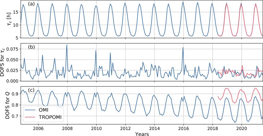
K. Sun et al.: Observational-data-driven emission and lifetime estimates over air basins 13317
time. Those originate from irregular features in the column– from the optimal estimation will effectively suppress noise
wind speed relationship (observable in Fig. 3) and tend to in the observed column–wind speed relationship.
be more significant when satellite coverage is low. Because In this optimal estimation setup, the 12 climatological
of the stochastic nature of atmospheric motion, those irregu- column–wind relationships are concatenated into a single
lar features randomly appear in a limited number of calendar observation vector, and the 12 climatological chemical life-
months, leading to wide spread of bootstrapping realizations times and emission rates are retrieved simultaneously as a 24-
and namely large uncertainties in emission rate and chemical element state vector. The fitted OMI- and TROPOMI-based
lifetime estimates. τc values with outlier calendar months removed (black sym-
We additionally remove “outlier” calendar months that bols in Fig. 6b and d) are averaged together and smoothed
would significantly alter the fitted τc and Q from the cli- by a first-order Savizky–Golay filter with a 3-month win-
matological column–wind speed relationship. These outlier dow (Savitzky and Golay, 1964). This smoothed curve is
months are often characterized by anomalously high NO2 used as the prior values of chemical lifetimes for both OMI
TVCDs over a few wind speed bins. For each calendar and TROPOMI. The prior value for the emission rates is a
month, the corresponding climatological month is processed constant 260 mol s−1 for all climatological months. The prior
twice, with and without that calendar month included in the error standard deviation is loosely set at 150 % for both Q
averaging. The differences of the fitted Q and τc the clima- and τc , and a time correlation scale of 1.5 months is as-
tological month with and without a specific calendar month sumed within the lifetime terms and the emission rate terms
are displayed in Fig. 5. The calendar month is excluded as an in the prior error covariance matrix. The model–observation
outlier if the absolute value of its impact on the climatolog- mismatch error depends on satellite retrieval error, the rep-
ical Q is larger than 70 mol s−1 or the absolute value of its resentativeness of satellite observation in the air basin, and
impact on the climatological τc is larger than 1.5 h. The long the chaotic nature of atmospheric motion. Little is known
record of OMI enables a second round of outlier removal, about the last two sources of error except that longer av-
whereby the climatology is averaged from a single month eraging time may reduce them, so we simplify the model–
(instead of 3-month window). It is impossible to do that for observation mismatch error as a single regularization factor
TROPOMI as 1 climatological month would only have 2–3 λ that presents its overall variance. Optimal λ values are de-
calendar months to average from. In this round, the max Q termined separately for OMI and TROPOMI by balancing
difference with and without including a calendar month is the norm of fitting residuals and the norm of the prior error-
still 70 mol s−1 , but the max τc difference is relaxed to 5 h. weighted deviation of the solution to the prior using the L
The excluded calendar months are highlighted by red dots in curve (Hansen and O’Leary, 1993). Details on the optimal
Fig. 5. More winter months are excluded due to lower cov- estimation setup are provided in Appendix B.
erage and consequently noisier column–wind speed relation- Figure 7 shows the posterior climatological emission rates
ship. 53 % of winter calendar months in the OMI record are Q (a and c) and chemical lifetimes τc (b and d) optimally
excluded, while the overall removal rate is 30 %. estimated using OMI (a and b) and TROPOMI (c and d)
After identifying and excluding the outlier calendar column–wind speed relationships. After taking into account
months, the climatological column–wind speed relationships the correlations between climatological months via Bayesian
are finalized, and the climatology of emission rates and optimal estimation, the errors are markedly reduced com-
chemical lifetimes are fitted again. The results are shown in pared with individual climatological month fittings shown in
Fig. 6. The fitting quality is significantly improved, as indi- Figs. 4 and 6. The climatological emission rates estimated
cated by the reduced variation of bootstrap realizations. from OMI data are higher than TROPOMI because overall
the OMI record covers more early years (2004–2021) than
3.3.2 Optimal estimation of climatological chemical TROPOMI (2018–2021), and the emission rate has been de-
lifetime creasing (see Sect. 4.4). The posterior climatological chemi-
cal lifetimes will be discussed in Sect. 4.2.
The climatological NOx chemical lifetimes fitted from the
previous step are still unsatisfactory due to remaining large 3.3.3 Optimal estimation of emission rates and
errors and correlation between fitted emission rates and chemical lifetimes for all calendar months
chemical lifetimes. For instance, the OMI-based chemical
lifetimes in climatological months April and September are Finally, the monthly NOx emission rate and chemical life-
unrealistically shorter than the summer months (Fig. 6b), time are retrieved from the column–wind speed relationships
which is inconsistent with the TROPOMI values (Fig. 6d) of all calendar months simultaneously in an optimal estima-
and corresponds to suspiciously high emission rates in those tion algorithm (see Appendix B for technical details). The
two climatological months (Fig. 6a). To further improve the prior values of monthly τc are taken from the OMI-based τc
climatology estimates, we incorporate the a priori informa- climatology due to its overall higher quality and longer tem-
tion that the climatology should vary smoothly over the year poral coverage (see Fig. 7b and d and further discussion in
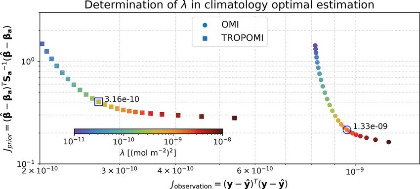
through a Bayesian optimal estimation. The regularization Sect. 4.2). In other words, the OMI-based posterior chemical
https://doi.org/10.5194/acp-21-13311-2021 Atmos. Chem. Phys., 21, 13311–13332, 2021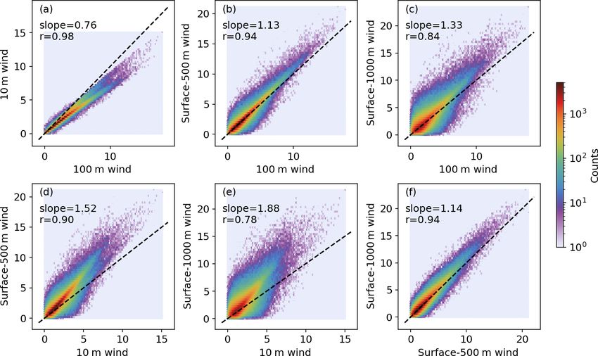
13318                              K. Sun et al.: Observational-data-driven emission and lifetime estimates over air basins

Figure 4. Fitting of the column–wind speed relationships for each climatological month for OMI (a, b) and TROPOMI (c, d). The black
symbols are fitted from real observed data, and the gray symbols are bootstrapping realizations.

Figure 5. Exclusion of outlier months (red) for OMI (a) and TROPOMI. Each dot locates the differences of Q and τc from the corresponding
climatological month fitting with and without a specific calendar month. The blue boxes show the boundaries delineating the maximum
tolerated Q and τc influences from each calendar month to their corresponding climatological month.

lifetimes in the 12 climatological months are used as the prior       4     Results
chemical lifetime in each calendar month for both OMI and
TROPOMI. The prior error of calendar month τc is assumed              4.1    Selection of air basin length scale
to be 30 %, autocorrelated with an interannual timescale of
1.5 years and an intra-annual timescale of 1.5 months. This
                                                                      Equation (5) expresses the dynamic lifetime of NOx in an air
prior regularization to the τc terms is instrumental in the suc-
                                                                      basin dimensionally as the ratio between a length scale L and
cessful retrieval of the emission rate Q. The prior values of
                                                                      wind speed. To assess the uncertainties induced by such sim-
monthly Q are estimated from an exponential function fitted
                                                                      plification, we conduct sensitivity studies using end-to-end
from the annually averaged JPL chemical reanalysis emis-
                                                                      emission rate and chemical lifetime estimations described
sion rates, and 100 % prior errors are used. No error corre-
                                                                      in Sect. 3.3 by switching wind speed options described in
lations are assumed among the Q terms and between Q and
                                                                      Sect. 2.3 and varying the prescribed values for L. The resul-
τc terms. This configuration maximizes the information con-
                                                                      tant OMI-based emission rates are compared with total sur-
tent of emission rates Q from observations while suppressing
                                                                      face NOx emission rates from the JPL chemical reanalysis.
excessive noise in the results.
                                                                      We choose OMI-based emission rates due to long-term con-
                                                                      sistency and large overlap with the JPL chemical reanalysis.

Atmos. Chem. Phys., 21, 13311–13332, 2021                                              https://doi.org/10.5194/acp-21-13311-2021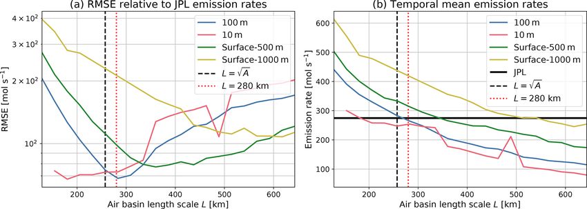
K. Sun et al.: Observational-data-driven emission and lifetime estimates over air basins                                             13319

Figure 6. Similar to Fig. 4, but after outlier month exclusion shown in Fig. 5.

Figure 7. Similar to Figs. 4 and 6, but using Bayesian optimal estimation incorporating the prior knowledge that the climatological emission
rates and lifetimes should vary smoothly.

The combined wind speed option and L value that gives the                 pares the temporally averaged emission rates. The optimal
closest agreement with the JPL chemical reanalysis monthly                L value, characterized by the lowest RMSE and the match-
emission rate is selected, as the overall accuracy of the JPL             ing of temporal mean emission rates to the JPL mean value,
chemical reanalysis is constrained by multiple observation                increases in the order of 10 m, 100 m, surface–500 m, and
datasets.                                                                 surface–1000 m wind, consistent with the overall magnitude
   Figure 8a shows the root mean square error (RMSE) be-                  of those four wind options. As shown in Fig. 2, those four
tween the OMI-based emission rates and corresponding JPL                  wind speeds are linearly well correlated. Therefore, the op-
chemical reanalysis values for 2005–2019, and Fig. 8b com-                timal L value scales with the wind strengths and partially

https://doi.org/10.5194/acp-21-13311-2021                                               Atmos. Chem. Phys., 21, 13311–13332, 2021
13320                                 K. Sun et al.: Observational-data-driven emission and lifetime estimates over air basins

Figure 8. (a) Root mean square error (RMSE) of OMI-based emission rates relative to the monthly JPL chemical reanalysis emission rates
for 2005–2019 when using 10, 100, surface–500 m, and surface–1000 m wind speeds as W in Eq. (5) and a range of L values. (b) Comparison
of the temporal mean emission rates estimated from those wind and length scale options with the mean JPL chemical reanalysis emission
rate. The square root of the air basin area is shown as the black vertical dashed line, and the selected air basin length scale (280 km) is shown
as the red vertical dotted line.

“absorbs” the systematic differences between wind speed op-                and 27 h in summer and winter in 2012 and 5.9 and 21 h
tions. We choose 100 m wind due to its low optimal RMSE                    in summer and winter 2017 using GEOS-Chem in China.
and better representation of horizontal advection than the                 Over the Netherlands, Zara et al. (2021) found that the win-
10 m wind. The basin length scale L is selected to be 280 km,              ter NOx lifetime decreased from 25 to 19 h and the summer
similar to the square root of the air basin area (257 km). One             NOx lifetime decreased from 9 to 8 h using the Chemistry
should note that this length scale is specific to the Po Valley            Land-surface Atmosphere Soil Slab (CLASS) model.
air basin and should be fixed in time. A length scale should                  The TROPOMI-based climatological chemical lifetimes
be similarly estimated before applying such a framework to                 are suspiciously low after September. As the NOx sinks are
other source regions.                                                      driven by ambient temperature and solar radiation, we do
                                                                           not expect lower chemical lifetimes in September–October
4.2   NOx chemical lifetimes                                               than June–July. This anomaly likely results from abnormal
                                                                           TROPOMI column–wind speed relationships characterized
The optimally estimated climatological chemical lifetimes,                 by high NO2 TVCDs in a few wind speed bins. Although
which are shown in Fig. 7b and d, are replotted in Fig. 9 to               the individual monthly column–wind speed relationship from
emphasize the confidence intervals and the prior values com-               OMI is noisier than TROPOMI (Fig. 3), the much longer
mon for OMI and TROPOMI. The TROPOMI-based chemi-                          OMI record (201 calendar months vs. 38 calendar months
cal lifetime estimates are consistently lower than the OMI-                for TROPOMI) enables more effective removal of outlier
based values, but the error bars overlap in climatological                 months and retrieval of climatological chemical lifetimes.
months January–July, indicating that the differences are not               As such, we focus on the OMI-based chemical lifetime cli-
significant. Because the OMI climatology spans 2004–2021                   matology for the following analysis. The NOx climatolog-
while the TROPOMI one spans 2018–2021, this difference                     ical chemical lifetimes are 5–6 h in summer and 15–20 h
implies a weak yet notable long-term decrease in NOx chem-                 in winter, generally consistent with CTM studies that con-
ical lifetime. This is likely due to the decrease in NOx emis-             sider NOx sinks comprehensively (Mijling and Van Der A,
sions (see Fig. 12) and consequently the shifting of chemical              2012; Stavrakou et al., 2013; Silvern et al., 2019; Shah et al.,
regimes away from NOx -saturated conditions (Martin et al.,                2020). The summertime NOx chemical lifetime is also close
2004). Shifting in summertime NOx chemical lifetime due                    to or slightly higher than other observational-data-driven es-
to a change in NOx abundance and chemical regimes has                      timates, mostly through fitting the downwind decay of NO2
been identified in North American cities using OMI obser-                  plumes (Valin et al., 2013; de Foy et al., 2015; Liu et al.,
vations and an EMG-based approach (Laughner and Cohen,                     2016; Goldberg et al., 2019a; Laughner and Cohen, 2019).
2019). Model studies indicated a similar NOx chemical life-                This is consistent with the modeling verification by de Foy
time change in polluted regions undergoing decreasing emis-                et al. (2014), which found the NOx chemical lifetime derived
sions. Using the GEOS-Chem CTM, Silvern et al. (2019)                      from the EMG-based approach to be biased low compared to
found that the annual mean tropospheric NO2 column life-                   the true lifetimes in the model simulations.
time over the contiguous US was 8.1 h in 2005 and 7.7 h in                    The OMI-based climatological chemical lifetimes in Fig. 9
2017. Shah et al. (2020) simulated NOx lifetime to be 6.1                  are then used as priors to derive chemical lifetimes in each

Atmos. Chem. Phys., 21, 13311–13332, 2021                                                    https://doi.org/10.5194/acp-21-13311-2021
K. Sun et al.: Observational-data-driven emission and lifetime estimates over air basins 13321 Figure 9. Prior (black) and posterior (blue for OMI and red for TROPOMI) climatological chemical lifetimes from optimal estimation. The prior chemical lifetimes are based on nonlinear fitting to the climatological column–wind speed relationships. The error bars indicate 95 % confidence intervals by bootstrapping the calendar months used to construct each climatological column–wind speed relationship. Figure 10. Time series of chemical lifetime (a), degrees of freedom for signal (DOFS) for chemical lifetime τc (b), and DOFS for emission rate Q (c) from the calendar-month-based optimal estimations using OMI (blue) and TROPOMI (red) monthly data. calendar month for both OMI and TROPOMI. The resul- ical lifetimes for calendar months are dominated by prior in- tant monthly NOx chemical lifetimes are shown in Fig. 10a. fluences from the climatological chemical lifetimes, which Note that the chemical lifetimes in Fig. 10a are retrieved reflects our trade-off between emission rates and chemical from column–wind speed relationships for each calendar lifetimes by applying relatively strong prior regularization to month, whereas the chemical lifetimes in Fig. 9 are retrieved τc in each calendar month. While the climatological chemical from column–wind speed relationships for each climatolog- lifetimes are also derived from observations, the lack of ob- ical month. The degrees of freedom for signal (DOFS) of servational constraints for the lifetime in each individual cal- retrieved emission rates and chemical lifetimes, shown by endar month makes them closely resemble the corresponding Fig. 10b and c, are the diagonal elements of the averaging climatological month values (i.e., the prior) and prevents us kernel matrix as given in Appendix B. The DOFS quantifies from further interpretation of these monthly lifetime values. the number of pieces of information retrieved from obser- The information on the retrieved emission rate Q that vations for a specific state vector element (Rodgers, 2000; is gained from observations, indicated by the correspond- Brasseur and Jacob, 2017). The observational information ing DOFS, is, however, high and close to unity (Fig. 10c). content of τc for each calendar month, as indicated by the This indicates that we can confidently retrieve emission rates DOFS, is only ∼ 0.02 (Fig. 10b). This implies that the chem- from the monthly column–wind speed relationships. The de- https://doi.org/10.5194/acp-21-13311-2021 Atmos. Chem. Phys., 21, 13311–13332, 2021
13322                              K. Sun et al.: Observational-data-driven emission and lifetime estimates over air basins

caying DOFS for OMI-based emission rates from 2004 to               sis reports 3.5 % of NOx emissions in the Po Valley from
2021 is likely due to the gradual increase in OMI radiance          soils. However, other top-down studies indicate that the soil
noise (Schenkeveld et al., 2017) and consequently increased         emissions may be underestimated in Europe, ranging from
uncertainties in OMI NO2 TVCD. The higher DOFS from                 14 % to 40 % (Visser et al., 2019, and references therein).
TROPOMI than OMI is also consistent with the instrument             Since the satellites observe emissions from all sources, the
performances.                                                       discrepancy may also be from missing soil NOx emissions in
                                                                    bottom-up inventories. The TROPOMI-based emission rates
4.3   Observational constraints on the NOx : NO2 ratio              show similar variation as OMI and the JPL chemical re-
                                                                    analysis, but tend to be lower than OMI in the cold months
Despite its limited effect on the estimates of NOx chemi-           and higher than OMI in the warm months. The calendar
cal lifetime and relative emission changes, the uncertainty         month chemical lifetimes retrieved from TROPOMI are sim-
of the NOx : NO2 ratio (φ in Eq. 5) will directly propa-            ilar to OMI (Fig. 10a), and hence the differences in OMI-
gate to the NOx emission rate estimates. We investigate the         and TROPOMI-based emission rates directly result from dif-
ground-based NOx : NO2 ratio measured at EEA sites as la-           ferences in their NO2 TVCDs. This is supported by Fig. 3;
beled in Fig. 11a. No ratio data are available in the most          when wind speed is controlled, the OMI TVCDs are higher
polluted Milan metropolitan area because only NO2 data are          in cold months, while the TROPOMI TVCDs are higher in
reported. Figure 11b shows the monthly distribution of the          warm months.
NOx : NO2 ratio in the Po Valley as grayscale background               Once the air basin length scale is selected (see Sect. 4.1),
and the monthly median values as a red line. The data cov-          the proposed satellite-data-driven framework can be used to
erage is sparse in 2015–2017, and no sensible temporal vari-        quantify rapid emission perturbations. The Po Valley region
ation can be identified. Consistent seasonal variation of the       experienced three major COVID-19 outbreaks, and the con-
NOx : NO2 ratio is observable in 2018–2021 with high values         dition is still evolving (Dong et al., 2020). All outbreaks trig-
(1.5–1.6) in the winter and low values (1.2–1.3) in other sea-      gered lockdown measures that are expected to reduce NOx
sons, with the caveat that the data after 2020 are not fully val-   emissions. However, the quantitative measure of net emis-
idated. The ratios in 2013 and 2014 show a similar seasonal         sion reduction due to the lockdowns is complicated by the
pattern but broader distributions and higher median values in       long-term decreasing trend and intra-annual variability. For
the warm months. Given this discontinuity, we cannot draw a         instance, the simple difference between 2020 and 2019 val-
conclusion about the interannual trend of the NOx : NO2 ra-         ues includes both the pandemic-induced emission changes
tio. Nonetheless, the seasonal pattern is robust and consistent     and the business-as-usual decrease. Leveraging the long and
with low photochemical reactivity in the winter. Therefore,         consistent OMI record, we train a statistical model to present
we average the monthly NOx : NO2 ratios in 2013–2014 and            the interannual and intra-annual variability using the OMI-
2018–2019 and use them as a climatology.                            based emission rates from January 2010 to December 2019
                                                                    (yellow shaded region in Fig. 13a):
4.4   NOx emission rates
                                                                    Q(t) =
                                                                        np
                                                                                                                            !
Figure 12 presents the monthly air-basin-scale emission rate            X           nh
                                                                                   X
                                                                                i

retrieved from OMI and TROPOMI column–wind speed re-                exp     ci t +     aj sin (2π tj ) + bj cos (2π tj ) + e , (6)
                                                                          i=0          j =1
lationships. The long-term trend and seasonality of OMI-
based emission rates generally match those from the JPL             where t is time measured in fractional years resolved by
chemical reanalysis (r = 0.40). The emission rates from             month, c, a, and b are model parameters, and e is an error
bottom-up inventories EDGAR, PKUNOx, and CEDS are                   term. The order of polynomial np = 3 and the number of har-
also shown in Fig. 12; EDGAR is only available as annual av-        monics nh = 4 are chosen through the Akaike information
erage. We use the surface total NOx emissions from the JPL          criterion (Akaike, 1974). The fitted model and 95 % confi-
chemical reanalysis, which does not include lightning (1.8 %        dence intervals are estimated using ordinary least squares
of surface total). According to the JPL chemical reanalysis,        and displayed in Fig. 13a and b. Because the model fitting
96.2 % of surface total NOx emissions are anthropogenic.            does not involve data before 2010 or after 2020, the model
All sectors from CEDS, EDGAR, and PKUNOx are used.                  line over those years is from extrapolation and character-
Although the PKUNOx and CEDS inventories are monthly,               ized by increasingly large uncertainties (i.e., broader confi-
their seasonality differs significantly from the OMI-based          dence intervals) as the range of projection grows. The well-
and JPL chemical reanalysis values. The interannual trends          documented emission perturbation during the 2008–2009 fi-
agree reasonably well between bottom-up inventories and             nancial crisis (Castellanos and Boersma, 2012) is evident in
top-down emission estimates (JPL chemical analysis and this         the discrepancy between model extrapolation and real emis-
study) in their overlapping periods, although the emission          sion rates (Fig. 13a). Similarly, since this statistical model
decrease trends are not as strong in the top-down estimates         is trained using data before the pandemic, the prediction
as in the bottom-up estimates. The JPL chemical reanaly-            in 2020 and beyond serves as a business-as-usual baseline.

Atmos. Chem. Phys., 21, 13311–13332, 2021                                           https://doi.org/10.5194/acp-21-13311-2021
K. Sun et al.: Observational-data-driven emission and lifetime estimates over air basins 13323 Figure 11. (a) Black circles are the locations of ground-based observation sites where NOx and NO2 data are available. TROPOMI NO2 TVCD from May 2018 to May 2019 oversampled to a 0.02◦ grid is illustrated in the background. (b) The background shows the density of available NOx : NO2 ratios from filtered hourly ground-based measurements. The red line shows the monthly median values. Figure 12. Po Valley NOx emission rates retrieved from OMI (blue circles) and TROPOMI (red squares) column–wind speed relationships in each calendar month. Monthly emission rates calculated from the JPL chemical reanalysis, EDGAR, PKUNOx, and CEDS inventories are shown as black, magenta, yellow, and cyan lines. The background color map indicates the prior error distributions normalized to the peak height of unity for each calendar month. Compared to just using a previous year or multiyear averaged emission reduction started in February 2020 and peaked in climatology as a reference (Goldberg et al., 2020; Liu et al., March 2020 at 42 %. The emission rate gradually recovered 2020; Bauwens et al., 2020), the model prediction incorpo- as the first outbreak was under control and reached 85 %– rates both the long-term trend and seasonality and is less 95 % of the pre-existing trajectory in June–September 2020. sensitive to noise in monthly estimates. The real emission Thereafter, the emission rate dropped twice as of July 2021, rates during the pandemic relative to the predicted emission reaching reductions of 38 % and 39 % relative to the no- rates are shown in Fig. 13c. Significant COVID-19-induced pandemic scenario in November 2020 and March 2021. https://doi.org/10.5194/acp-21-13311-2021 Atmos. Chem. Phys., 21, 13311–13332, 2021
13324                                K. Sun et al.: Observational-data-driven emission and lifetime estimates over air basins

Figure 13. (a) The blue dots show the monthly OMI-based emission rates. The black solid and dashed lines show the prediction and 95 %
confidence intervals using the model as in Eq. (6). Only data points for 2010–2019 (yellow shade) are used to fit the model. Prediction values
outside this range are extrapolations. Panel (b) is similar to (a) but focused on the period after 2019. (c) The bars show real 2020–2021
emission rates relative to the predicted emission rates. The yellow and red lines show Google and Apple mobility indicators.

These reductions correspond to the second and third out-                 between the mobility indicators and OMI-based net emission
breaks with the subsequent controlling measures. The emis-               changes. Discrepancies are noted in April 2020 and January
sion rates in January–February and May–June 2021 seem to                 2021, when the mobility indicators stayed low after major
be back to the expected normal, highlighting the evolving                control measures, but the NOx emissions recovered quicker.
nature of pandemic-induced emission perturbations. Over-                 We speculate that this is the impact of industrial NOx emis-
all, the real annual emission of 2020 is estimated to be 22 %            sions that are not well represented by the human mobility
lower due to the net effect of the COVID-19 pandemic in the              indicators.
Po Valley air basin.
   We further correlate the COVID-19-induced NOx emis-
sion changes with the qualitative indicators of human activi-            5    Conclusions and discussion
ties estimated by the mobility of Google (Google LLC, 2021)
and Apple (Apple, 2021) users. The Google mobility is mea-               We present a satellite-data-driven framework to rapidly quan-
sured by aggregated Google user activity levels for the cat-             tify NOx emission rates over an air basin and demonstrate it
egories grocery and pharmacy, parks, transit stations, work-             in the Po Valley, Italy. Monthly emission rates and chemical
places, and retail and recreation relative to a baseline period          lifetimes of NOx are retrieved from observed column–wind
during 3 January–6 February 2020. Google mobility reported               speed relationships, wherein the NOx column abundance is
for six Italian regions in the Po Valley air basin, includ-              represented by OMI and TROPOMI NO2 TVCD observa-
ing Piedmont, Lombardy, Veneto, Liguria, Emilia–Romagna,                 tions, and the wind speed is obtained from ERA5 reanalysis.
and Friuli–Venezia Giulia, is averaged. The Apple mobility               To regularize the retrieval, we derive a NOx chemical life-
is measured by Apple user activity levels in driving and tran-           time climatology and use it as prior information. The NOx
sit modes over the entirety of Italy relative to the baseline            chemical lifetime is 5–6 h in summer and 15–20 h in winter.
on 13 January 2020. Both Google and Apple mobility indi-                 Our observation-based emission rate estimates are consistent
cators are in daily native resolution and averaged weekly to             with top-down and bottom-up inventories and can be quickly
remove day-of-week effects. The result is shown in Fig. 13c.             updated as the method only depends on satellite and reanal-
The relative NOx emission changes and the mobility indi-                 ysis data. Leveraging the long and consistent OMI record, a
cators consistently show the three troughs corresponding to              statistical model is trained to predict the business-as-usual
large outbreaks. The impacts of the second and third out-                trajectory without the pandemic. Compared with this tra-
breaks were lower than the first one, which is also consistent           jectory, the real 2020–2021 emission rates show three dis-
                                                                         tinctive dips that correspond to tightened COVID-19 control

Atmos. Chem. Phys., 21, 13311–13332, 2021                                                  https://doi.org/10.5194/acp-21-13311-2021
K. Sun et al.: Observational-data-driven emission and lifetime estimates over air basins 13325 measures and reduced human activities. The overall net NOx emission reduction due to the COVID-19 pandemic is esti- mated to be 22 % in 2020 with maximum reduction in March, followed by November. The pandemic-induced emission re- duction continued in March–April 2021. Only observations under modest wind (3–8 m s−1 ) are used, so there is an implicit assumption that NOx emissions under modest wind can represent all wind conditions. Since NOx sources in air basins are mostly anthropogenic, this as- sumption is deemed to be valid. In addition, the satellite ob- servations are made in the early afternoon local time, so the retrieved emission rates may not necessarily represent the di- urnal mean emission rate. This is a common limitation of all observational-data-driven approach, and we note that the overall emission rate level is anchored to the overall emission rate level of the JPL chemical reanalysis, which is spatiotem- porally complete, through the selection of basin length scale L. The uncertainties of the retrieved monthly emission rates may also originate from the systematic biases of NO2 TVCD products, but the relative emission variations should be insen- sitive to the observational biases. Updated satellite products (e.g., the version 2 TROPOMI NO2 product to be released in 2021) can be readily adopted. The monthly climatological NOx : NO2 ratio derived from ground-based observation net- works is used to convert NO2 abundance to NOx abundance, which improves upon the fixed value used in previous stud- ies (Beirle et al., 2011; Valin et al., 2013; de Foy et al., 2015; Liu et al., 2016). However, uncertainty remains from con- tamination of NO2 in situ measurements (Visser et al., 2019) and the representativeness of the surface-based NOx : NO2 ratio to the column-integrated one due to proximity to emis- sion sources and local ozone titration. Moreover, a long-term trend in NOx : NO2 may exist, as observed in the Nether- lands by Zara et al. (2021), although biases in NOx : NO2 have limited impacts on chemical lifetime and relative emis- sion change estimates. The seasonal variability of estimated NOx emissions is determined by the seasonal variabilities of NO2 TVCD, chemical lifetime, and the NOx : NO2 ratio. We attempt to characterize these variabilities using as much ob- servational data as possible, and yet future investigations are still needed. The general framework is not limited to NO2 and NOx in the Po Valley air basin, but can be applied to investigating the emissions and lifetimes of other short-lived species in other geographical regions. https://doi.org/10.5194/acp-21-13311-2021 Atmos. Chem. Phys., 21, 13311–13332, 2021
You can also read