OMPS LP Version 2.0 multi-wavelength aerosol extinction coefficient retrieval algorithm - Recent
←
→
Page content transcription
If your browser does not render page correctly, please read the page content below
Atmos. Meas. Tech., 14, 1015–1036, 2021
https://doi.org/10.5194/amt-14-1015-2021
© Author(s) 2021. This work is distributed under
the Creative Commons Attribution 4.0 License.

OMPS LP Version 2.0 multi-wavelength aerosol extinction
coefficient retrieval algorithm
Ghassan Taha1,2 , Robert Loughman3 , Tong Zhu4 , Larry Thomason5 , Jayanta Kar5,6 , Landon Rieger7 , and
Adam Bourassa7
1 Universities  Space Research Association (USRA), Greenbelt, MD, USA
2 NASA    Goddard Space Flight Center, Greenbelt, MD, USA
3 Department of Atmospheric and Planetary Sciences, Hampton University, Hampton, VA, USA
4 Science Systems and Applications Inc., Greenbelt, MD, USA
5 Science Directorate, NASA Langley Research Center, Hampton, VA, USA
6 Science Systems and Applications Inc., Hampton, VA, USA
7 Institute of Space and Atmospheric Studies, University of Saskatchewan, Saskatoon, Saskatchewan, Canada

Correspondence: Ghassan Taha (ghassan.taha@nasa.gov)

Received: 13 August 2020 – Discussion started: 4 September 2020
Revised: 1 December 2020 – Accepted: 30 December 2020 – Published: 10 February 2021

Abstract. The OMPS Limb Profiler (LP) instrument is de-           accuracies and precisions close to 10 % and 15 %, respec-
signed to provide high-vertical-resolution ozone and aerosol      tively, while the 675 nm relative accuracy and precision are
profiles from measurements of the scattered solar radiation       on the order of 20 %. The 510 nm extinction coefficient is
in the 290–1000 nm spectral range. It collected its first Earth   shown to have limited accuracy in the SH and is only recom-
limb measurement on 10 January 2012 and continues to pro-         mended for use between 20–24 km and only in the Northern
vide daily global measurements of ozone and aerosol pro-          Hemisphere. The V2.0 retrieval algorithm has been applied
files from the cloud top up to 60 and 40 km, respectively.        to the complete set of OMPS LP measurements, and the new
The relatively high vertical and spatial sampling allow detec-    dataset is publicly available.
tion and tracking of sporadic events when aerosol particles
are injected into the stratosphere, such as volcanic eruptions
or pyrocumulonimbus (PyroCb) events. In this paper we dis-
cuss the newly released Version 2.0 OMPS multi-wavelength         1     Introduction
aerosol extinction coefficient retrieval algorithm. The algo-
rithm now produces aerosol extinction profiles at 510, 600,       1.1    The importance of stratospheric aerosol
674, 745, 869 and 997 nm wavelengths. The OMPS LP Ver-                   measurements
sion 2.0 data products are compared to the SAGE III/ISS,
OSIRIS and CALIPSO missions and shown to be of good               Observations of the stratospheric aerosol layer were first pro-
quality and suitable for scientific studies. The comparison       vided by Junge et al. (1961) using balloon-borne measure-
shows significant improvements in the OMPS LP retrieval           ments, showing a layer extending from 15 to 25 km altitude
performance in the Southern Hemisphere (SH) and at lower          with a peak at 20 km. Further measurements established that
altitudes. These improvements arise from use of the longer        the main composition of the aerosol in this layer is 75 % sul-
wavelengths, in contrast with the V1.0 and V1.5 OMPS              furic acid and 25 % water (SPARC, 2006; Deshler, 2008).
aerosol retrieval algorithms, which used radiances only at        The stratospheric aerosol budget is dominated by natural
675 nm and therefore had limited sensitivity in those re-         sources, where volcanic injections of SO2 and aerosol di-
gions. In particular, the extinction coefficients at 745, 869     rectly into the lower stratosphere stand out as the largest
and 997 nm are shown to be the most accurate, with relative       source over the past decades. Carbonyl sulfide (OCS) makes
                                                                  the second largest contribution to the aerosol layer. These

Published by Copernicus Publications on behalf of the European Geosciences Union.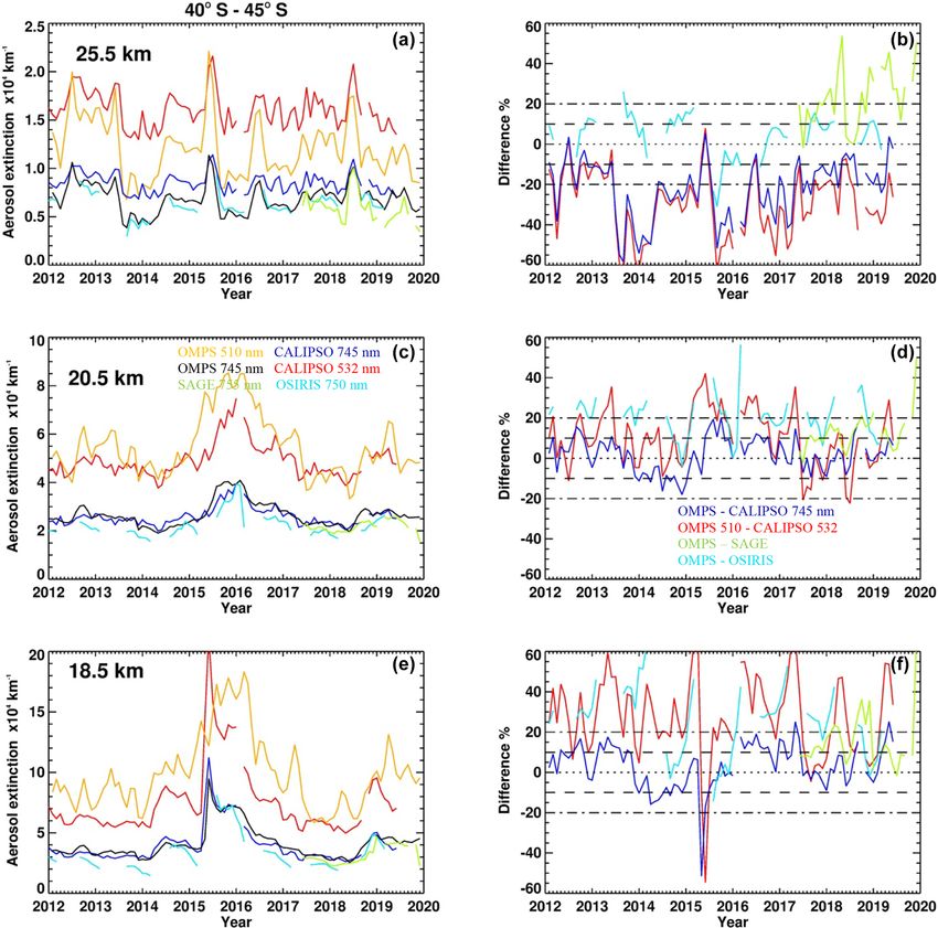
1016            G. Taha et al.: OMPS LP Version 2.0 multi-wavelength aerosol extinction coefficient retrieval algorithm

sulfur species originate at the Earth’s surface in a variety of    1.2     Overview of stratospheric aerosol measurement
reduced forms (including CS2 , DMS and H2 S) before oxida-                 types
tion in the atmosphere (Kremser et al., 2016). Other sources
of stratospheric aerosol include the transport of tropospheric     A comprehensive review of the wide variety of stratospheric
aerosol across the tropical tropopause through large con-          aerosol measurements is outside the scope of this study.
vective systems such as the Asian monsoon (Vernier et al.,         (The interested reader should refer to Sect. 4 of Kremser
2011a; Thomason and Vernier, 2013). In recent years, there         et al., 2016, for example.) This section will briefly name
has been evidence that pyrocumulonimbus (PyroCb) events            some key types of measurements that are useful for deter-
during large wildfires can inject smoke aerosol into the           mining various properties of stratospheric aerosols and high-
stratosphere, which can be comparable to volcanic aerosol          light some advantages and disadvantages of each technique.
injections in terms of impact on the stratosphere (Fromm et        This overview will focus primarily on the space-based re-
al., 2010; Peterson et al., 2018; Yu et al. 2019; Torres et al.,   mote sensing methods that are discussed further in Sects. 3–
2020).                                                             5, especially those that are used directly to assess the perfor-
   Stratospheric aerosols can have a direct impact on Earth’s      mance of the OMPS LP aerosol extinction retrieval.
climate system by affecting its radiative balance, and they
also play an important role in the chemical and dynamical          1.2.1    In situ and ground-based measurements
processes related to ozone destruction in the stratosphere
(Hofmann and Solomon, 1989; Solomon, 1999; Zhu et al.,             In situ measurements mainly provide information about the
2018). Powerful volcanic eruptions such as Mount Pinatubo          stratospheric aerosol size distribution, from which moments
in 1991 can increase the stratospheric sulfur burden by sev-       (such as surface area density and volume density) can be de-
eral orders of magnitude over the pre-eruption levels, which       rived. These instruments directly sample stratospheric air, us-
can last for several years and lead to stratospheric warming       ing a balloon-borne or aircraft platform. Examples include
and tropospheric cooling (Robock, 2000; Deshler, 2008). A          the optical particle counters (OPCs; Hofmann and Deshler,
volcanic eruption like Pinatubo can also lead to cooling of        1991; Jaeger and Deshler, 2002), the airborne focused cavity
the surface temperature on the order of a few tenths of a de-      aerosol spectrometer (FCAS; Jonsson et al., 1995), and the
gree (Robock and Mao, 1995). It was also shown that the            nucleation-mode aerosol size spectrometer (NMASS; Brock
background stratospheric aerosol layer is persistently vari-       et al., 2000). Size information can be obtained for particles
able, modulated by weaker volcanic eruptions, thus affecting       in the size range 0.05–10 µm, depending on the particular in-
the global surface temperature (Solomon et al., 2011; Vernier      strument. In situ measurements can provide higher temporal
et al., 2011b). Furthermore, Santer et al. (2014) identify sta-    and spatial sampling than other techniques during a measure-
tistically significant anti-correlations between observations      ment campaign. But the cost and effort associated with such
of stratospheric aerosol optical depth and satellite-based es-     a campaign limit this method to intensive case studies, rather
timates of tropospheric temperature, and they show that cli-       than providing broad temporal and spatial coverage.
mate model simulations without the effects of early 21st cen-         Ground-based lidars also make measurements of strato-
tury volcanic eruptions overestimate the tropospheric warm-        spheric aerosols (Poole and McCormick, 1988; Chouza et al.,
ing observed since 1998. Other investigations confirm that         2020). In this case, the signal consists of photons backscat-
early 21st century volcanic eruptions are one of several fac-      tered by stratospheric aerosols, and therefore the measure-
tors that affect the decreased warming observed during that        ments provide the backscattering coefficient of the particles.
period (relative to expectations based on continued growth         This is typically converted into an aerosol extinction coeffi-
of the greenhouse gases in the atmosphere) (Schmidt et al.,        cient, using an assumed “lidar ratio” as the conversion fac-
2014; Medhaug et al., 2017). Stratospheric aerosol has also        tor. The signal-to-noise ratio of a single lidar measurement
been used as a tracer to study stratospheric dynamics (Trepte      is generally low, which requires a combination of many indi-
and Hitchman, 1992; Jaeger, 2005; Fairlie et al., 2014). Over      vidual shots to produce useful retrievals. Ground-based lidars
the past few years, there has been a rising interest in the        are typically stationary, so they provide information at just
geoengineering concept for solar radiation management, by          one location, but they can provide high temporal sampling
injecting aerosol into the stratosphere (Rasch et al., 2008),      and good vertical resolution.
for which a basic understanding of the present stratospheric
aerosol layer is essential. A review paper by Kremser et           1.2.2    Space-based occultation measurements
al. (2016) concluded that it is critical to maintain continu-
ous observational records to detect unpredictable events (like     The primary space-based method for characterizing strato-
large volcanic eruptions) or unexpected developments (such         spheric aerosol is the occultation method, in which pho-
as non-volcanic processes like strong PyroCb events that re-       tons emitted by a bright source of radiation are transmitted
sult in changes in stratospheric aerosol levels), noting that      through the atmosphere as the source rises or sets through
observations are critical for testing the reliability of climate   the atmosphere (as viewed by the instrument). These line-
models.                                                            of-sight transmission profiles are then converted into vertical

Atmos. Meas. Tech., 14, 1015–1036, 2021                                             https://doi.org/10.5194/amt-14-1015-2021
G. Taha et al.: OMPS LP Version 2.0 multi-wavelength aerosol extinction coefficient retrieval algorithm                     1017

profiles of extinction coefficient for the various atmospheric    1.2.4    Space-based lidar measurements
constituents, including aerosol extinction coefficient. The
transmission measurement is essentially “self-calibrating,”       Spaceborne backscatter lidar measurements by Cloud-
and this fact (combined with the high signal-to-noise ratio       Aerosol Lidar and Infrared Pathfinder Satellite Observation
provided by a bright radiation source) leads to retrievals with   (CALIPSO) are also used to explore the stratospheric aerosol
high precision and accuracy. However, the locations and fre-      layer (Thomason et al., 2007a; Vernier et al., 2009; Kar et al.,
quency of occultation events are entirely determined by the       2019). The description given in Sect. 1.2.1 for ground-based
orbit of the instrument, which limits the coverage that can be    lidars generally applies to the spaceborne lidars as well. The
achieved.                                                         main difference is that an orbiting lidar provides the addi-
   Most occultation measurements for stratospheric aerosol        tional advantage of mobility (near global coverage in the case
studies use solar occultation (with the sun as the source         of CALIPSO). The spaceborne CALIPSO lidar instrument is
of photons). Examples of this technique include the Strato-       used in this study and is described further in Sect. 3.3.
spheric Aerosol Measurement (SAM II; McCormick et al.,
1982), the Stratospheric Aerosol and Gas Experiment (SAGE         1.2.5    Summary of available measurements
II; Chu et al., 1989) and SAGE III (Thomason and Taha,
                                                                  In 2017, accurate solar occultation measurements of strato-
2003), Polar Ozone and Aerosol Measurement (POAM II
                                                                  spheric aerosols resumed after the deployment of SAGE
and III; Lumpe et al., 2002), the Halogen Occultation Ex-
                                                                  III on the International Space Station (ISS; Cisewski et al.,
periment (HALOE; Hervig et al., 1996), the Improved Limb
                                                                  2014). Combined with the ongoing OSIRIS and CALIPSO
Atmospheric Spectrometer (ILAS I and II; Hayashida et al.,
                                                                  missions, we now have coincident stratospheric aerosol mea-
2000; Saitoh et al., 2006), and the Measurement of Aerosol
                                                                  surements from several space-based platforms. The structure
Extinction in the Stratosphere and Troposphere Retrieved by
                                                                  of this paper is as follows: in Sect. 2 we provide a brief de-
Occultation (MAESTRO; McElroy et al., 2007; Sioris et al.,
                                                                  scription of the OMPS LP instrument and V2.0 algorithm
2010). Aerosol extinction profiles were also measured by the
                                                                  changes. The correlative satellite aerosol measurements are
stellar occultation instrument Global Ozone Monitoring by
                                                                  described further in Sect. 3. Section 4 describes the validation
Occultation of Stars (GOMOS; Vanhellemont et al., 2010).
                                                                  methodology. The comparison results are shown in Sect. 5,
The particular solar occultation instrument used in this study
                                                                  followed by conclusions in Sect. 6.
(the SAGE III instrument on the ISS) is described further in
Sect. 3.1.
                                                                  2     OMPS LP measurements and algorithm description
1.2.3   Space-based limb scattering measurements
                                                                  2.1     Instrument review
In recent years, several limb scattering (LS) measurements
have become available, including SAGE III limb (Rault             The OMPS LP sensor images the Earth limb by pointing aft
and Taha, 2007), Optical Spectrograph and InfraRed Im-            along the spacecraft flight path to measure the sunlit por-
ager System (OSIRIS; Llewellyn et al., 2004; Bourassa et          tion of the globe without directly observing the sun. The
al., 2007), SpectroMeter for Atmospheric CHartographY             sensor employs three vertical slits separated horizontally to
(SCIAMACHY; Taha et al., 2011; von Savigny et al., 2015;          provide near-global coverage in 3–4 d and more than 7000
Malinina et al., 2018) and OMPS LP (Gorkavyi et al., 2013;        profiles a day. The instrument measures limb scattering ra-
Rault and Loughman, 2013). These instruments measure              diance at the 290–1000 nm wavelength range and the 0–
the radiance scattered by the limb of the atmosphere. The         80 km altitude range. The instrument is installed in a fixed
strength of the stratospheric aerosol signal in these radiances   orientation relative to the spacecraft, which flies in a sun-
depends on several aerosol properties, including the aerosol      synchronous ascending orbit with 13:30 Equator crossing
refractive index, shape, size and number density. These prop-     time. As a result, the observed single-scattering angle (SSA)
erties affect both the aerosol phase function and aerosol ex-     varies along the orbit, where the Northern Hemisphere (NH)
tinction coefficient, both of which influence the aerosol sig-    observations correspond to forward-scattered solar radiation,
nal present in the measured limb radiance.                        and the Southern Hemisphere (SH) observations correspond
   This study evaluates the OMPS LP V2.0 aerosol extinc-          to backscattered radiation. Therefore, the aerosol scattering
tion retrieval algorithm, which estimates the aerosol extinc-     signal is much larger in NH than in the SH, resulting in a
tion coefficient based on the measured LS radiance as de-         sampling of the aerosol phase function magnitude varying
scribed in Sect. 2.2. The resulting extinction coefficients are   by a factor of 50 over the course of OMPS orbit (Lough-
compared to the OSIRIS aerosol extinction product, which is       man et al., 2018). OMPS LP is scheduled to fly on the
described further in Sect. 3.2.                                   NOAA JPSS-2, JPSS-3 and JPSS-4 satellites, to extend the
                                                                  stratospheric aerosol measurements into the next couple of
                                                                  decades. (These satellite launches are currently targeted for
                                                                  2022, 2026 and 2031, respectively.)

https://doi.org/10.5194/amt-14-1015-2021                                            Atmos. Meas. Tech., 14, 1015–1036, 2021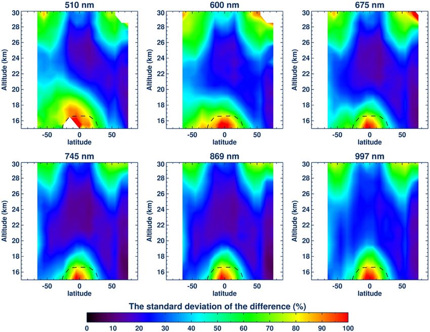
1018            G. Taha et al.: OMPS LP Version 2.0 multi-wavelength aerosol extinction coefficient retrieval algorithm

2.2     OMPS LP V2.0 algorithm improvement                             The Earth’s surface is modeled as a Lambertian surface
                                                                    (for which a fraction, R, of the incident downward radiation
The Version 2.0 (V2.0) OMPS LP aerosol extinction retrieval         is reflected as isotropic, unpolarized upward radiance field
algorithm builds upon the Version 1.0 (V1.0) and Version 1.5        at each point). The value of R is determined by requiring
(V1.5) algorithms, which were described in Sect. 4 of Lough-        that I c0 (λ, h) = I m (λ, h) at h = 40.5 km (Loughman et al.,
man et al. (2018) and Sects. 2 and 3 of Chen et al. (2018), re-     2018). An approximate ozone correction is also applied to
spectively. We therefore begin by briefly reviewing the V1.0        the model radiances to correct for possible ozone error, as de-
and V1.5 algorithms in Sect. 2.2.1 and defining the key vari-       scribed in Sect. 4.3 of Loughman et al. (2018). To reduce the
ables used. This is followed by Sect. 2.2.2, which details the      sensitivity of the algorithm to a variety of interfering factors,
algorithm updates made to produce V2.0.                             the radiances are normalized with respect to tangent height h.
                                                                    The measured altitude-normalized radiance (ANR) is defined
2.2.1    Review of the V1.0 and V1.5 OMPS LP                        as ρ m (λ, h) = I m (λ, h)/I m (λ, hn ), with hn , namely the nor-
         algorithms                                                 malization tangent height, set to a value of 40.5 km in the
                                                                    V1.0 and V1.5 algorithms. The value of hn is generally se-
Unlike solar occultation, limb scattering retrievals require
                                                                    lected as a compromise between two competing interests. It
complex forward model calculations, and the aerosol re-
                                                                    should be as high as possible to minimize the atmospheric
trieval in particular requires assumptions of aerosol refrac-
                                                                    aerosol extinction at hn , but not so high that the radiance at hn
tive index and size parameters. Previous versions of the
                                                                    is poorly characterized (due to residual stray light contamina-
OMPS LP aerosol retrieval algorithm were mainly designed
                                                                    tion, low signal-to-noise ratio, etc.). Analogous expressions
for minimizing the errors of ozone profiles and level-1 radi-
                                                                    define ρ c (λ, h) and ρ c0 (λ, h) based on the calculated radi-
ance diagnostics. The V1.0 and V1.5 algorithms use OMPS
                                                                    ance profiles.
LP radiance measurements, I m (λ, h), for a range of tangent
                                                                       As a final step, the ANR values are combined to pro-
heights, h, at a single wavelength (λ = 675 nm) to estimate
                                                                    duce the aerosol scattering index (ASI), which serves as the
the aerosol extinction profile. This wavelength was selected
                                                                    measurement vector y in the retrieval. The measured ASI is
to be near the Chappuis band that is used to retrieve the
                                                                    defined as y m (λ, h) = [ρ m (λ, h)−ρ c0 (λ, h)]/ρ m (λ, h), with
ozone profile in the visible region, for which the OMPS LP
                                                                    similar definitions for y c (λ, h) and y c0 (λ, h). Since the V1.0
radiances are best characterized. The algorithm assesses the
                                                                    and V1.5 algorithms use a single wavelength, this notation
measurements by comparison to two analogous sets of calcu-
                                                                    can be abbreviated to y m (λ, hi ) = y m i , with a similar abbre-
lated radiances, I c (λ, h) and I c0 (λ, h). These calculated ra-
                                                                    viation y c (λ, hi ) = y ni used to represent the ASI calculated
diance profiles are generated by the Gauss–Seidel limb scat-
                                                                    based on the model atmosphere after n iterations of the re-
tering (GSLS) radiative transfer model (RTM) (Loughman
                                                                    trieval algorithm.
et al., 2004) for the same viewing and solar illumination
                                                                       The V1.0 and V1.5 algorithms use the Chahine nonlin-
conditions that existed when I m (λ, h) was measured. The
                                                                    ear relaxation method (Chahine, 1970) to derive the aerosol
model atmospheres used (described further below) are iden-
                                                                    extinction coefficient (which represents the state vector, x)
tical for these two calculations, with one exception: in the
                                                                    based on the measurement vector y defined above. The state
case of I c0 (λ, h), the model atmosphere contains no aerosols,
                                                                    vector is updated iteratively as shown in Eq. (1):
while the I c (λ, h) model atmosphere contains the first-guess
aerosol profile.                                                                   ym
   The model atmosphere consists of static atmospheric tem-         x n+1
                                                                      i   = x ni    i
                                                                                        = x ni fin .                              (1)
                                                                                   y ni
perature and pressure profiles derived from the operational
geopotential height product provided by the NASA Global             In this expression, x n+1 is the state vector at altitude zi , and
                                                                                          i
Modeling and Assimilation Office (GMAO). The algorithm              n + 1 is the number of iterations. The measurement vector
uses the McPeters and Labow (2012) ozone climatology and            ym                                                   n
                                                                      i is the ASI at tangent height h = zi , while y i is the cal-
the PRATMO photochemical box model NO2 climatology                  culated ASI based on the extinction profile corresponding
(McLinden et al., 2000) to define the model atmosphere. The         to the nth iteration. As shown in Eq. (1), the retrieval cre-
first-guess aerosol extinction profile, x 0 , is defined based on   ates the updated aerosol extinction coefficient estimate x in+1
a single SAGE climatological profile. Aerosols are assumed          by multiplying the previous estimate, x ni , by the factor fin .
to consist of spherical liquid sulfate particles (75 % H2 SO4 )     The V1.0 algorithm constrains the value of fin to lie be-
with index of refraction m = 1.448 + 0i (Yue and Deepak,            tween 0.2 and 2.0 and sets the number of iterations to N = 3.
1983; Wang et al., 1996). In the V1.0 algorithm, the aerosol        These constraints were primarily motivated by caution in the
size distribution (ASD) is assumed to be a bi-modal log-            early stages of developing the aerosol extinction retrieval al-
normal distribution (Loughman et al., 2018); this was up-           gorithm, when the stability of the retrieval was relatively
dated to a gamma distribution in V1.5 (Chen et al., 2018).          untested. The V1.5 algorithm relaxed these constraints some-
Mie scattering theory is used to calculate the aerosol phase        what, using N = 4 and allowing fin values between 0.2 and
function based on the assumed ASD and optical properties.           3.0.

Atmos. Meas. Tech., 14, 1015–1036, 2021                                                   https://doi.org/10.5194/amt-14-1015-2021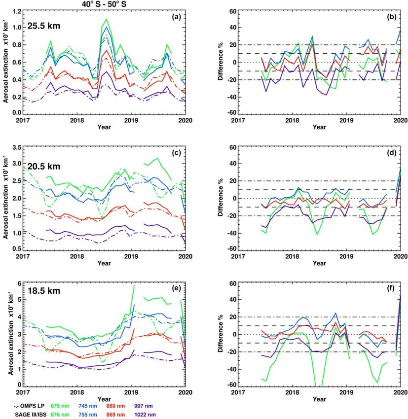
G. Taha et al.: OMPS LP Version 2.0 multi-wavelength aerosol extinction coefficient retrieval algorithm                        1019

2.2.2   Updates made for the V2.0 OMPS LP algorithm

Since the limb scattering radiances at visible and near-
infrared wavelengths are very sensitive to aerosol proper-
ties, the V2.0 OMPS LP aerosol algorithm is modified to
include multiple wavelengths in this spectral region, simi-
lar to the SAGE III aerosol channels (Thomason and Taha,
2003). The V2.0 algorithm uses OMPS LP measurements at
wavelengths 510, 600, 675, 745, 869 and 997 nm, selected to
minimize the effect of gaseous absorption, with the excep-
tion of 600 nm, which will be used primarily for diagnostics.
Each wavelength is retrieved independently, as described in
                                                                  Figure 1. Panel (a) is a plot of retrieved OMPS LP aerosol extinc-
the preceding section leading to Eq. (1). Taha et al. (2011)
                                                                  tion profiles (×104 km−1 ) colored by wavelength for event 26 in
showed that, because of its strong weighting function or Ja-      the SH measured on 12 April 2018. Panel (b) is the aerosol scatter-
cobian matrix, retrieving aerosol profiles at longer wave-        ing index (ASI) or measurement vectors (y) for the same event. The
lengths can improve the quality of the profile in the South-      dashed line is the tropopause altitude.
ern Hemisphere, where OMPS LP observes backscattered
radiation, and extend the retrieval further down in altitude.
The Jacobian matrix quantifies the changes in the radiance        ily done for speed purposes: scalar (unpolarized) radiance
with respect to the aerosol extinction. Multiple wavelength       calculations are considerably faster than their vector (po-
aerosol measurements can also provide limited information         larized) counterparts, and the resulting change in ρ c (λ, h)is
about aerosol particle size and can be used to identify cloud     very small. Recent calculations performed for a RTM com-
presence. Notice that the 997 nm radiance measurements are        parison project (Zawada et al., 2020) allow the ρ c (λ, h) val-
only available after 26 November 2013.                            ues computed by the scalar and vector versions of GSLS to be
   The assumed ASD is the same in V2.0 as in V1.5, but the        compared, for a variety of atmospheres and illumination con-
single first-guess aerosol extinction profile has been replaced   ditions. For the relevant wavelengths (500 nm and greater),
by a first-guess climatology that varies with wavelength, lat-    these values agree to within 1 % or better at 20 km and within
itude and season, again based on the SAGE aerosol data            2 % or better at 10 km.
record. The V2.0 algorithm further relaxes the constraints           Figures 1 and 2 illustrate the contrasting effect of the scat-
that were previously applied to the Chahine iteration results:    tering angle on the measurement vector and subsequent re-
N = 5 and fin has an upper bound of 10.0 and no lower             trieved aerosol extinction profiles at different wavelengths.
bound. The V2.0 algorithm also checks for convergence after       Figure 1 shows that at scattering angle 154◦ , wavelengths
each iteration, rather than always performing the stated num-     shorter than 745 nm have poor sensitivity to aerosol, which
ber of iterations: iterations end when the retrieved aerosol      limits the accuracy and altitude range of the OMPS LP SH
extinction changes by < 2 % at 20 km or when it reaches the       aerosol retrieval. In contrast, the longer wavelengths show
maximum number of iterations. The planned V2.1 release            high sensitivity to aerosol, thus improving the retrieval sig-
next year will use modified convergence criteria that check       nificantly at lower altitudes. Notice that the cloud at 10.5 km
for multiple altitudes.                                           is only observed by the longer wavelengths. Figure 2 illus-
   Limb scattering instruments such as OSIRIS, SCIA-              trates the strong sensitivity of all six wavelengths to aerosol
MACHY and OMPS LP suffer from increased stray light at            when the scattering angle is small. In the NH, the OMPS
increasing wavelength and altitude due in part to diminishing     LP measurement vector for all wavelengths is positive for all
scattered signal (Jaross et al., 2014; Rieger et al., 2019). To   altitudes, and the aerosol retrieval quality does not vary sig-
reduce the stray light effect on the retrieval at longer wave-    nificantly with wavelength. Notice that all retrieved aerosol
lengths, hn was lowered to 38.5 km in V2.0 (from the 40.5 km      wavelengths can detect the cloud layer evident as enhanced
value used in previous versions). The GSLS radiative trans-       extinction near 10.5 km.
fer model used in the V2.0 algorithm was also updated as
described by Loughman et al. (2015). The main improve-
ment associated with this change involves the use of several      3     Correlative aerosol measurements
zeniths to calculate the multiple-scattering source function
along the limb line of sight, which improves the radiance         3.1    SAGE III/ISS
calculations near the terminator. Unlike the V1.0 and V1.5
algorithms, the V2.0 GSLS model also includes refraction          The SAGE series of instruments started with the Strato-
in the line-of-sight calculation. The V2.0 algorithm also ex-     spheric Aerosol Monitor (SAM) in 1975, SAM II in 1978
cludes polarization (which had been included in the V1.5 ra-      (McCormick et al., 1982), SAGE I in 1979, SAGE II (Chu et
diance calculations). The exclusion of polarization is primar-    al., 1989) in 1984 and SAGE III Meteor 3M (M3M; Thoma-

https://doi.org/10.5194/amt-14-1015-2021                                             Atmos. Meas. Tech., 14, 1015–1036, 2021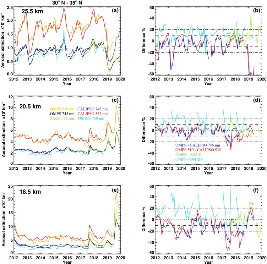
1020             G. Taha et al.: OMPS LP Version 2.0 multi-wavelength aerosol extinction coefficient retrieval algorithm

                                                                   found mean differences of less than 10 % in the tropics to
                                                                   mid-latitudes, with larger biases at higher latitudes and at al-
                                                                   titudes outside the main aerosol layer.
                                                                      More recently, the V7 OSIRIS retrieval was introduced,
                                                                   which combines information from measurements at 470,
                                                                   675, 750 and 805 nm to produce multi-wavelength aerosol
                                                                   extinction retrievals. The expanded wavelength usage re-
                                                                   duces biases caused by measurement geometry and improves
                                                                   the retrieval coverage and quality in the upper troposphere
                                                                   and lower stratosphere (UT–LS) region. The V7 algorithm
                                                                   also uses a modified version of the Chen et al. (2016) cloud
                                                                   detection algorithm (for polar stratospheric cloud (PSC) de-
Figure 2. Same as Fig. 1 but for event 150 in the NH.
                                                                   tection and general cloud screening). Rieger et al. (2019) re-
                                                                   port agreement at the 10 % level between SAGE II and the
son and Taha, 2003) in 2001, spanning over 26 years. On 19         Version 7 OSIRIS retrieval, with exceptions at high altitudes,
February 2017, SAGE III was launched to the International          which exhibit low bias due to sensitivity to stray light and
Space Station (ISS) to resume the SAGE series of measure-          nonzero aerosol in OSIRIS normalization altitudes. Over-
ments. It provides high-resolution vertical profiles of aerosol    all, the V7 product agreement with coincident SAGE data
extinction at multiple wavelengths; the molecular densities of     is comparable to the V5.07 performance, while the agree-
ozone, nitrogen dioxide and water vapor; and profiles of tem-      ment with the CALIPSO-GOCCP product (Chepfer et al.,
perature, pressure and cloud presence. The aerosol extinction      2010) is improved relative to V5.07. However, Kovilakam
is computed as a residual after accounting for Rayleigh scat-      et al. (2020) noted that OSIRIS extinction is consistently
tering and gaseous absorption, and thus, the retrieval makes       higher than SAGE II in the lower stratosphere with the dif-
no prior assumptions of the aerosol size or phase function.        ference exceeding 30 % near the tropopause when comparing
However, the technique is limited in coverage and number           monthly means.
of profiles, to typically about 30 per day. The SAGE III/ISS
                                                                   3.3   CALIPSO
retrieval algorithm is essentially the same as its predeces-
sor on the Meteor 3M platform. The quality of the SAGE             The spaceborne lidar on CALIPSO which was launched in
III on Meteor 3M aerosol data was evaluated by Thomason            April 2006 provides global measurements of vertically re-
and Taha (2003) and Thomason et al. (2007b, 2010). These           solved aerosol- and cloud-attenuated backscatter coefficients
studies found that the aerosol extinction measurements’ ac-        at 532 and 1064 nm (Winker et al., 2010). Significant im-
curacy and precision are on the order of 10 % between 15 and       provement in calibration in V4 of CALIPSO data products
25 km, with the exception of 601 and 675 nm above 20 km,           makes it possible to obtain extinction coefficients in the
which exhibit substantial bias that was caused by the ozone        stratosphere even with limited signal-to-noise ratio. The V1
clearing. A recent study by Wang et al. (2020) about SAGE          Level-3 CALIPSO stratospheric aerosol profile product was
III/ISS ozone validation also stated that an error in ozone cor-   produced using only the nighttime measurements, and sub-
rection caused an underestimation of the aerosol retrievals at     stantial spatial (vertical averaging to 900 m, 5◦ latitude bins,
wavelengths near the Chappuis band at altitudes where the          20◦ longitude bins) and temporal (monthly) averaging were
aerosol loading is minimal. Thomason et al. (2021) also re-        applied. A constant lidar ratio (extinction-to-backscatter ra-
ported a defect in these wavelengths below 20 km due to an         tio) of 50 sr was used to obtain the extinction profiles, which
error caused by the O4 cross section used in V5.1.                 is a typical value used for stratospheric aerosol background
                                                                   conditions (Kremser et al., 2016). The extinction profiles
3.2    OSIRIS
                                                                   were retrieved using two different methods. In the “back-
OSIRIS is an instrument that measures vertical profiles of         ground” mode, all detected cloud and aerosol layers were re-
limb-scattered sunlight from the upper troposphere into the        moved and thin cirrus clouds within a few kilometers above
lower mesosphere. It was launched on February 2001 on              the tropopause were filtered using a threshold on the vol-
board the Odin satellite and continues to take measurements        ume depolarization ratio (Kar et al., 2019). In the “all-aerosol
to the present. The instrument measures ozone, aerosol and         mode”, all layers detected as aerosols in the stratosphere
NO2 profiles. Initial (V5.07) aerosol retrievals were obtained     were retained, and thin cirrus were filtered using a threshold
by combining measurements at 470 and 750 nm and were               on the attenuated color ratio. In this work, we use the gridded
reported as aerosol extinction profiles at 750 nm. Rieger et       extinction profiles from the all-aerosol mode for consistently
al. (2015) compared coincident aerosol extinction observa-         comparing with OMPS. It should be noted that in this mode,
tions by interpolating the SAGE II 525 and 1020 nm chan-           the cirrus cloud removal is not as efficient as in the back-
nels to the OSIRIS extinction wavelength of 750 nm. They           ground mode.

Atmos. Meas. Tech., 14, 1015–1036, 2021                                             https://doi.org/10.5194/amt-14-1015-2021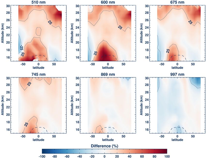
G. Taha et al.: OMPS LP Version 2.0 multi-wavelength aerosol extinction coefficient retrieval algorithm                        1021

   Initial validation of V1.0 CALIPSO L3 532 nm strato-             volcanic or PyroCb plumes, we filtered the data by removing
spheric aerosol profiles is described by Kar et al. (2019).         the extinction coefficient at and below cloud-top height only
This study concluded that CALIPSO agrees well with SAGE             if the reported cloud-top height is in the troposphere. SAGE
III/ISS aerosol, with CALIPSO about 25 % higher between             III is filtered for cloud contamination by using only data with
20–30 km in the tropics. However, the difference with SAGE          an extinction ratio of 510 to 1022 nm greater than 2 (Thoma-
III/ISS at the middle to high latitudes and low altitudes was       son and Vernier, 2013), while OSIRIS and CALIPSO provide
substantially larger, often exceeding 100 %.                        cloud-screened data.

4   Data comparison methodology                                     5     Results

In order to evaluate the accuracy of OMPS LP aerosol V2.0           5.1    Algorithm internal consistency
retrievals, we have used a variety of methods. This includes
comparison with the space-based instruments SAGE III/ISS,           So as to estimate the uncertainty of the assumed aerosol size
OSIRIS and CALIPSO, as well as performing internal con-             distribution and phase function, we compare measurements
sistency tests, which can quantify the uncertainty of the           taken at similar locations but with a different viewing geom-
aerosol model assumptions and the diffuse upwelling radi-           etry. Such measurements take place at high latitudes during
ance effect. To provide detailed assessment of OMPS per-            the summer of both hemispheres, when the OMPS orbit al-
formance at different altitudes, latitudes and times, we use        lows observations of a given latitude in both the ascending
two different approaches; coincident observation compari-           and descending nodes. The ascending and descending nodes
son and zonal mean climatology comparison. While the first          provide two daily observations of the same latitude, but with
approach is used to eliminate any geographical and time bi-         different scattering angles. The main assumption is that, if the
ases, the latter is proved to be useful for monitoring the health   retrieved aerosol values are different when the instrument is
and stability of the instrument and retrieval algorithm under       measuring the same air mass but with different scattering an-
different conditions and periods. However, zonally averaged         gle, then there is an error in the assumed phase function and
comparisons can produce large biases following large vol-           ASD model. As shown by Rieger et al. (2019), the ASD er-
canic eruptions, where the aerosol load is high and spatially       rors can introduce seasonal variations that correlate well with
inhomogeneous, and therefore coincident comparison is pre-          the SSA. Herein, we compare the daily zonal mean aerosol
ferred under these conditions (Rieger et al., 2019). The per-       climatology between ascending and descending nodes in the
cent difference is defined as                                       Northern Hemisphere, where the aerosol signal is stronger.
                                                                       Figure 3 is a scatter plot of the difference between ascend-
                 OMPS − reference                                   ing and descending zonal mean aerosol extinction coefficient
difference =                        × 100,                   (2)
               (OMPS + reference)/2                                 in the Northern Hemisphere between 60–90◦ N, plotted as a
                                                                    function of the difference of the SSA of the ascending and de-
where reference is the correlative measurement of aerosol           scending nodes at three different altitudes. The figure shows
extinction. All correlative aerosol profiles were interpolated      that at 20.5 km, the V2.0 algorithm has very little, if any, sen-
to 1 km vertical intervals, matching OMPS LP-reported al-           sitivity to the aerosol model errors. At 16.5 km, the depen-
titudes. Zonal mean climatologies were constructed using            dency of the aerosol retrieval on the scattering angle shows
monthly mean profiles within 5 or 10◦ latitude bins.                a linear trend of ≈ 0.25 % per degree for 745 and 869 nm
   For all comparisons shown in this paper, the center slit         and 0.5 % per degree for 675 nm. The trend is almost dou-
aerosol retrieval is used since it has the most accurate ra-        bled to −1 % per degree at 25.5 km, although it is distorted
diometric calibration and stray light corrections (Jaross et        by sensor noise and inhomogeneity of the aerosol loading
al., 2014). The OMPS LP algorithm identifies cloud-top              above the Junge layer at northern high latitudes, especially
height using the cloud detection method described in Chen et        when events occur inside the polar vortex where the aerosol
al. (2016). However, this algorithm also flags aerosols from        extinction is very low (Thomason and Poole, 1993). Never-
fresh volcanic eruptions or PyroCb events. OMPS LP V2.0             theless, the increase in the difference per unit of difference
data files now contain both cloud-filtered and unfiltered data,     in SSA suggests that the aerosol model used in the retrieval
as well as separate fields containing cloud height and type.        is less representative of the aerosol measured at this altitude.
Cloud type classifies the identified cloud as cloud, enhanced       Similar analyses made by Rieger et al. (2019) have shown
aerosol or PSC. The enhanced aerosol definition requires the        that the OSIRIS V7.0 aerosol extinction SSA dependence is
cloud altitude to be at least 1.5 km above the tropopause. The      0.5 % per degree.
PSC definition requires the cloud altitude to be at least 4 km
above the tropopause and the ancillary temperature at the
cloud altitude to be less than 200 K. Users may wish to use
both cloud height and cloud type flags to filter the data based
on their own needs. To avoid removing aerosols from fresh

https://doi.org/10.5194/amt-14-1015-2021                                              Atmos. Meas. Tech., 14, 1015–1036, 2021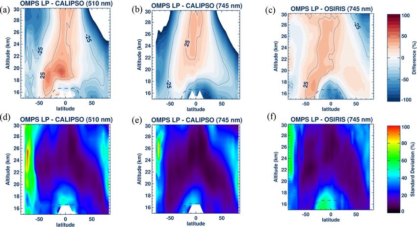
1022             G. Taha et al.: OMPS LP Version 2.0 multi-wavelength aerosol extinction coefficient retrieval algorithm

                                                                     Therefore, any observed differences outside the tropics are
                                                                     uncorrelated with cloud presence.

                                                                     5.3     Comparison of OMPS LP with SAGE III/ISS

                                                                     5.3.1    Coincidence comparison

                                                                     To evaluate the quality of OMPS LP aerosol retrieval with
                                                                     SAGE III, we use a coincidence criterion of same calendar
                                                                     day measurements, 1lat = ±3◦ and 1long = ±10◦ , which is
                                                                     selected to minimize the effect of spatial and temporal differ-
                                                                     ences between the two instruments. Coincidence pairs are av-
                                                                     eraged over 10 (Figs. 5, 7 and 8) or 40◦ (Fig. 6) latitudes bins
                                                                     covering the first 2 years of SAGE III/ISS measurements.
                                                                        Figure 5 depicts the mean OMPS LP and SAGE III/ISS
                                                                     aerosol extinction profiles for the set of coincident measure-
                                                                     ments, binned in 10◦ latitude bins, shown at selected alti-
                                                                     tudes for four different wavelengths. In general, OMPS LP
                                                                     and SAGE III extinction values show similar latitudinal dis-
Figure 3. Scatter plot of the difference between ascending and de-   tribution and are well within 20 % of each other for most
scending aerosol extinction coefficient zonal means (%) for 675      altitudes, with 869 nm showing the best agreement of bet-
(black), 745 (blue) and 869 nm (red) vs. the difference of single-   ter than 10 %. At 18.5 km in the SH tropics, OMPS aerosol
scattering angle (SSA) of the ascending and descending measure-
                                                                     is systemically higher than SAGE III, mostly influenced by
ments at 25 (top), 20.5 (middle) and 16.5 km (bottom). Measure-
                                                                     cloud presence at lower altitudes. The OMPS 675 nm extinc-
ments where the SSA difference is less than 6◦ are for zonal mean
latitude 90–80◦ N, SSA difference of 6–25◦ is for 80–70◦ N and       tion shows a negative bias at 18.5 km that increases with in-
SSA difference of 25–36◦ is for 70–60◦ N.                            creasing latitudes in the SH, where OMPS LP observes the
                                                                     backscatter solar radiation, and the attenuation of Rayleigh
                                                                     radiation is substantial below 20 km at 675 nm.
5.2    The diffuse upwelling radiance (DUR)                             Figure 6 is a summary plot of the mean difference between
       uncertainties                                                 OMPS and SAGE III coincidences for wavelengths 510, 600,
                                                                     675, 745, 869 and 997 nm. In general, 869 nm is the best
As described in Sect. 2.2.1, the aerosol retrieval algorithm         OMPS-retrieved wavelength relative to SAGE III with dif-
uses a simple Lambertian model of the reflecting surface to          ferences of 5 % or less for most altitudes and latitudes. Other
estimate an effective scene reflectivity (R). It does not mean       wavelengths agree with SAGE III to within 10 %. Exceptions
the Earth’s surface reflectivity, since the scene can contain        to this occur at high altitudes (above ≈ 28 km) where the
clouds or aerosols. Although the sensitivity of the aerosol          aerosol loading is minimal, and near the tropopause, which
retrieval to diffuse upwelling radiance (DUR) uncertainties          is affected by cloud contamination. The 510 and 600 nm
is reduced significantly by using normalized radiances (Flit-        OMPS extinction values have a slightly larger bias of 20 %
tner et al., 2000; Loughman et al., 2018), the error associated      in the tropics. This is due to the ozone interference in both
with assuming the Lambertian surface is difficult to estimate        OMPS and SAGE III 600 nm aerosol retrievals. The 997 nm
and possibly not negligible. In order to quantify DUR uncer-         OMPS extinction values have a systematic bias of −10 % be-
tainties, we compare OMPS LP daily zonal mean climatol-              tween 60◦ S and 20◦ N, caused by stray light contamination
ogy for R values less than 0.3 (cloud free) and greater than         in the OMPS measurements. Unlike the other wavelengths,
0.3 (bright or cloudy). Figure 4 is a plot of the percent dif-       the 997 nm laboratory characterization is poor, and its stray
ference between the two aerosol climatologies at three dif-          light correction, therefore, has lower quality (Jaross et al.,
ferent wavelengths. The three figures show a very similar            2014). In the SH, 510 nm shows a large positive bias relative
picture: very large differences below the tropopause in the          to SAGE III below 18 km. This is an artifact in the OMPS
tropics, where the cirrus clouds are more frequent and 5 %           retrieval algorithm, which often results in noisy and large
positive bias above 20 km, just over that cloudy region. The         extinction values when the measurement vector is too small
5 % bias may be caused by scattered light originating from           relative to gaseous absorption and Rayleigh scattering (see
cirrus clouds near the tropopause, which was not properly            Fig. 12).
accounted for in the radiative transfer model (which simply             It is worth noting that the best agreement between OMPS
used a bright Lambertian surface at sea level). Outside the          and SAGE is found in the NH, where OMPS observes in for-
tropics, the mean value of R is generally greater than 0.3,          ward scattering and the weighting function is strong for all
with strong seasonal dependence that peaks in the winter.            wavelengths. In that region, the agreement is mostly within

Atmos. Meas. Tech., 14, 1015–1036, 2021                                               https://doi.org/10.5194/amt-14-1015-2021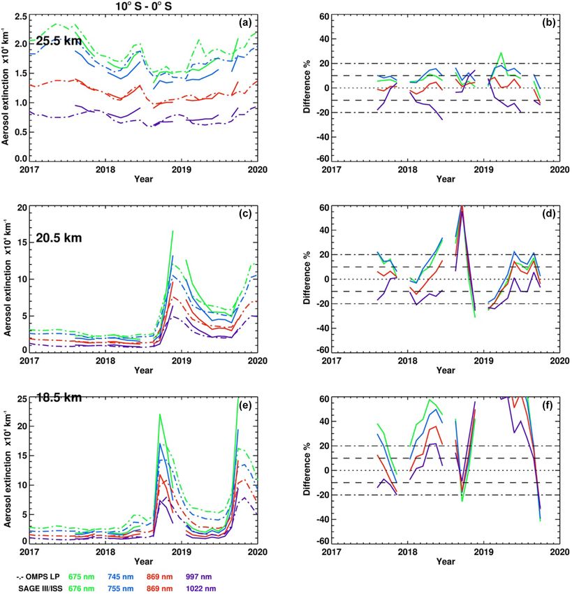
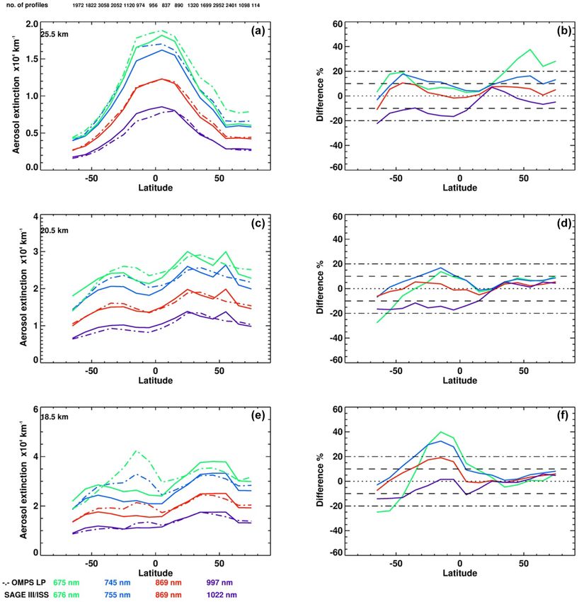
G. Taha et al.: OMPS LP Version 2.0 multi-wavelength aerosol extinction coefficient retrieval algorithm                                   1023

Figure 4. Panels (a) through (c) show the difference between the aerosol climatology when reflectivity is greater than 0.3 and when reflectivity
is less than 0.3. Extinction climatology at 745, 869 and 997 nm. The dashed line is tropopause altitude. The contour line shows differences
greater than ±5 %.

Figure 5. Panels (a), (c) and (e) are OMPS v2.0 (dash) and SAGE III (solid) aerosol extinction coefficient (×104 km−1 ) at 25.5, 20.5
and 18.5 km, for 675 (green), 745 (blue), 869 (red) and 997 nm (violet). Panels (b), (d) and (f) are the percent difference between the two
measurements. The number of coincidences for each zone is shown in the left top panel.

https://doi.org/10.5194/amt-14-1015-2021                                                      Atmos. Meas. Tech., 14, 1015–1036, 2021
1024             G. Taha et al.: OMPS LP Version 2.0 multi-wavelength aerosol extinction coefficient retrieval algorithm

Figure 6. Summary plot of the average percent difference between OMPS LP and SAGE III profiles in percent at three different latitudinal
zones for six wavelengths: 510 (orange), 600 (yellow), 675 (green), 745 (blue), 869 (red) and 997 nm (violet).

5 % for an altitude between 14 and 22 km. Above 24 km,                spheric variability. In general, the standard deviation is 15 %–
the observed biases for 510, 600, 675 and, to some extent,            20 % for altitudes that show good agreement with SAGE III
745, 869 and 997 nm gradually increase with altitude, mainly          (Fig. 7). The large standard deviation of ≈ 50 % at high al-
caused by instrument noise and errors under low-aerosol con-          titude is due to instrument noise and low aerosol loading.
ditions, although OMPS assumed aerosol size model uncer-              Below 20 km, the standard deviations for the shorter wave-
tainty also contributes to the larger differences.                    lengths increase to 50 %, caused by the OMPS LP reduced
   Figure 7 summarizes the quality of OMPS LP aerosol ex-             accuracy. In the UT–LS, the standard deviation is > 50 %
tinction at six retrieved wavelengths, showing the zonally            due to larger dynamical variability, especially during peri-
averaged mean differences between OMPS LP and SAGE                    ods when dispersal of plumes due to volcanic eruptions and
III aerosol (in percent). Below 25 km, the differences be-            other events causes longitudinal variations, as well as cloud
tween OMPS LP and SAGE III are largely driven by OMPS                 interference.
weighting functions or Jacobians. The weaker Jacobians for               Based on the comparison with SAGE III, we can estimate
short wavelengths under backscatter conditions in the SH and          the OMPS aerosol retrieval relative accuracy to be ≈ 10 %
below 20 km lead to limited accuracy, while stronger Jaco-            for 745, 869 and 997 nm in the stratosphere and 20 % for
bians at the longer wavelengths improve its accuracy signif-          675 nm above 20 km and in the NH. The 510 and 600 nm
icantly (Taha et al., 2011; Rieger et al., 2019). Overall, the        retrievals have limited accuracy in the SH and 25 % relative
shorter wavelengths (510, 600 and 675 nm) are biased low              accuracy at altitudes between 20–26 km and in the NH. Fur-
against SAGE III with a difference greater than 25 % below            thermore, the standard deviation can be used to determine the
20 km in the SH. In addition, these short wavelengths exhibit         retrieval relative precision, which can be estimated to be bet-
pronounced large aerosol in the tropics below 20 km caused            ter than 15 % for the longer wavelengths and close to 20 %
by the algorithm’s reduced accuracy when the measurement              for wavelengths less than 745 nm. The real precision is prob-
vector is very small. The agreement is well within 25 % at the        ably better than the quoted values since the calculated stan-
altitude range 20–25 km and better in the NH. Above 25 km,            dard deviation includes atmospheric variability and both in-
the comparison between the two instruments is poor, caused            struments’ biases, none of which was removed (Rault and
by either SAGE III ozone correction errors and/or OMPS re-            Taha, 2007; Wang et al., 2020).
duced sensitivity to aerosol at these short wavelengths. The
best agreement between OMPS and SAGE III can be seen at               5.3.2   Zonal mean comparison
869 and 997 nm, where they are mostly within 10 % of each
other for all altitudes and latitudes. The 745 nm OMPS ex-
                                                                      In order to investigate the OMPS LP retrieval performance
tinction agrees with SAGE to within 15 % everywhere except
                                                                      under different seasonal or geographical conditions, we com-
for the SH tropics below 18 km.
                                                                      pare the OMPS LP monthly zonal mean time series with the
   The standard deviation shown in Fig. 8 is influenced by
                                                                      SAGE III/ISS monthly zonal mean time series for four wave-
several factors: OMPS LP uncertainties such as measurement
                                                                      lengths at three different altitudes. The comparison is also
noise, forward model errors and retrieval algorithm sensitivi-
                                                                      divided into three different regions, the SH (Fig. 9), tropics
ties, in addition to SAGE III/ISS’s own uncertainty and atmo-
                                                                      (Fig. 10) and NH (Fig. 11). In general, the agreement be-

Atmos. Meas. Tech., 14, 1015–1036, 2021                                                 https://doi.org/10.5194/amt-14-1015-2021
G. Taha et al.: OMPS LP Version 2.0 multi-wavelength aerosol extinction coefficient retrieval algorithm 1025 Figure 7. Mean differences between OMPS LP and SAGE III extinctions as a function of latitude and altitude at 510, 66, 675, 745, 869 and 997 nm, zonally averaged at 10◦ latitudes. The contour line shows differences greater than ±25 %, and dashed line is the tropopause altitude. Positive differences (in percent) indicate the OMPS LP values are higher than SAGE III/ISS. Figure 8. Same as Fig. 7 but for the 1 − σ standard deviation or spread of difference between OMPS LP and SAGE III. https://doi.org/10.5194/amt-14-1015-2021 Atmos. Meas. Tech., 14, 1015–1036, 2021
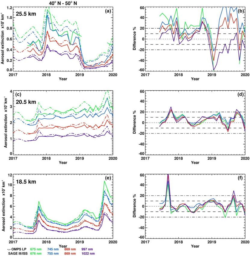
1026             G. Taha et al.: OMPS LP Version 2.0 multi-wavelength aerosol extinction coefficient retrieval algorithm

Figure 9. Panels (a), (c) and (e) are OMPS LP (dashed) and SAGE III/ISS (solid) aerosol extinction monthly zonal mean at 675, 745, 869
and 997 nm, latitude zone 40–50◦ S for altitudes 25.5 (top), 20.5 (middle) and 18.5 km (bottom), from 2017 to 2019. Panels (b), (d) and (f)
are the percent difference.

tween the two instruments in the SH is mostly within 10 %–              quency of measurements for each instrument. Still, the dif-
20 %. The 675 nm extinction at 20.5 km is a notable excep-              ference between the two measurements was mostly within
tion, as the OMPS LP aerosol extinction values drop signif-             20 % in the aftermath of this volcanic eruption. At 18.5 km,
icantly when the SSA is greater than 145◦ , and the attenu-             the difference is often greater than 20 %, reaching more than
ation of Rayleigh scattering below 20 km becomes signifi-               60 % following the subsidence of the volcanic plume. The
cant. This behavior appears as an apparent seasonal pattern,            reason for such large differences is unclear as OMPS LP still
in which the OMPS LP/SAGE III difference becomes much                   shows elevated aerosol levels when SAGE III measurements
larger during SH winter months. It is therefore recommended             indicate that the aerosol values are back to pre-eruption lev-
that OMPS aerosol measurements at λ ≤ 675 nm should be                  els, although spatial variability and spatial resolutions can
excluded when SSA is greater than 145◦ below 21 km.                     contribute to such large differences. SAGE III aerosol ex-
   A similar agreement is found in the tropics, at or above             tinction profiles are produced on a 0.5 km grid with an esti-
20.5 km, with the exception of the first few months follow-             mated vertical resolution of 0.7 km (SAGE III ATBD, 2002;
ing the Aoba volcanic eruption in July 2018, where OMPS                 Thomason et al., 2010) while OMPS LP vertical sampling
LP initially reported higher aerosol extinction than SAGE               is 1.0 km with an instantaneous resolution of 1.5 km (Jaross
III. This might be caused by the different coverage and fre-            et al., 2014). Bourassa et al. (2019) compared nearby OMPS

Atmos. Meas. Tech., 14, 1015–1036, 2021                                                   https://doi.org/10.5194/amt-14-1015-2021
G. Taha et al.: OMPS LP Version 2.0 multi-wavelength aerosol extinction coefficient retrieval algorithm                   1027

Figure 10. Same as Fig. 9 but for latitude zone 10–0◦ S.

LP and SAGE III/ISS aerosol profiles following the after-         aerosol loading was very high and spatially inhomogeneous.
math of the British Columbia fires in 2017. They showed that      Spatial inhomogeneity also caused a large bias after 2018
both instruments have very similar layered vertical structure     following the sharp drop in aerosol extinction at 25.5 km.
and magnitude. However, they noted that some differences          While the OMPS assumed ASD model may contribute to
in layer height and magnitude can be expected from differ-        the larger differences at 25.5 km, instrument noise and cal-
ing vertical resolutions. Another possible explanation is that    ibration errors are also more significant under low-aerosol
OMPS LP cloud clearing can be incomplete, and residual            conditions. OMPS LP 997 nm is affected by stray light con-
cloud contamination can contribute to the large differences       tamination at the normalization altitudes in the NH high lati-
near the tropopause. The best agreement between the two in-       tudes, which might explain the negative bias during 2019. On
struments can be found at 25.5 km, well within 10 %.              the other hand, SAGE III ozone correction uncertainty near
   In the NH, all OMPS LP wavelengths show similar robust         the Chappuis band can cause a dip in SAGE III aerosol ex-
agreement to SAGE III, mostly within 10 %, since OMPS LP          tinction measurements at 676 nm. In particular, the SAGE III
observes in the forward scattering and all wavelengths are        676 nm values at 25.5 km are either zero or negative during
strongly sensitive to aerosol (Fig. 11). A notable exception is   2019 when the measured aerosol is at its lowest levels in the
the first couple of months of the August 2017 Canadian Py-        NH during the short lifetime of ISS SAGE III.
roCb period and the June 2019 Raikoke eruption, when the

https://doi.org/10.5194/amt-14-1015-2021                                           Atmos. Meas. Tech., 14, 1015–1036, 2021
1028 G. Taha et al.: OMPS LP Version 2.0 multi-wavelength aerosol extinction coefficient retrieval algorithm
Figure 11. Same as Fig. 9 but for latitude zone 40–50◦ N.
5.4 Comparison of OMPS LP with OSIRIS and approach the ends of their lives, it is now more critical than
CALIPSO ever to extend the stratospheric aerosol record that has been
developed from SAGE–OSIRIS–CALIPSO into OMPS LP–
In this section, we compare OMPS LP aerosol at 510 and SAGE III/ISS records.
745 nm with V7 OSIRIS at 750 nm and V1 L3 CALIPSO Figures 12, 13 and 14 show OMPS LP, SAGE III/ISS,
at both 532 and 745 nm. CALIPSO 532 nm extinction (all- OSIRIS and CALIPSO zonally averaged monthly mean
aerosol mode) is converted to 745 nm using an Ångström aerosol extinction coefficient at three different altitudes in
exponent of 1.9, similar to the Ångström exponent for the the SH, tropics and NH, respectively, spanning a period be-
OMPS assumed aerosol model. We also included SAGE tween 2012 and 2019. The right panel is the mean difference
III/ISS measurements at 755 nm as an independent reference, in percent between OMPS LP and all instruments for the
since SAGE measurements are widely considered to be the same altitudes and latitudes. In general, OMPS LP, OSIRIS,
most accurate stratospheric aerosol dataset (SPARC, 2006; CALIPSO and SAGE III aerosol measurements are closely
von Savigny et al., 2015; Kremser et al., 2016; Thomason et matched at all altitudes, showing enhanced aerosol follow-
al., 2018; Kar et al., 2019). Although coverage and sampling ing the eruptions of Nabro (June 2011), Kelut (February
differences can make such comparisons difficult, it provides 2014), Calbuco (April 2015), Aoba (July 2018), Raikoke
a chance to evaluate the entire OMPS LP data record rela- (June 2019) and Ulawun (August 2019), as well as the Cana-
tive to these two datasets. As both OSIRIS and CALIPSO dian fires (August 2017). At 25.5 km in the tropics, OMPS
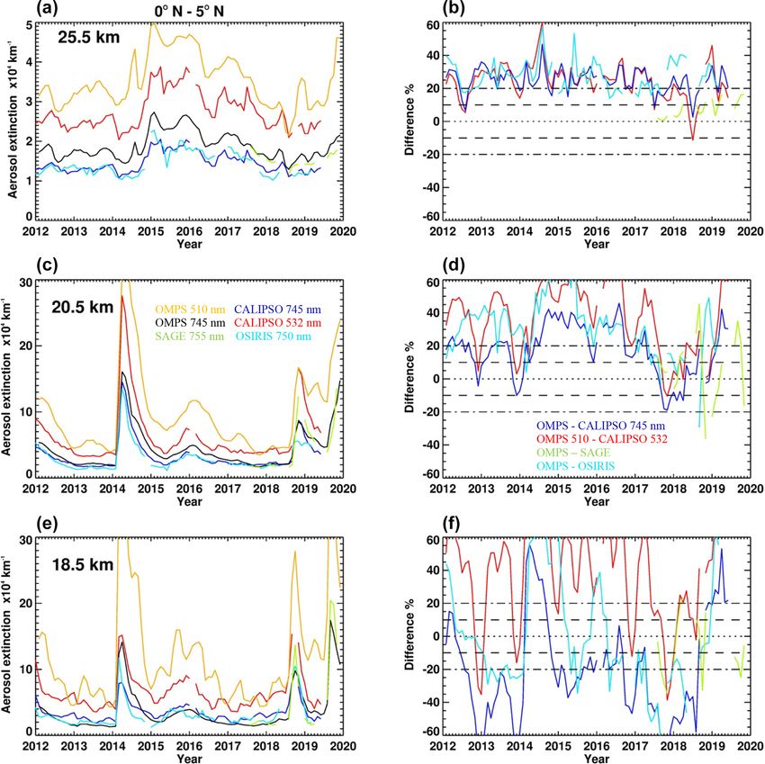
Atmos. Meas. Tech., 14, 1015–1036, 2021 https://doi.org/10.5194/amt-14-1015-2021G. Taha et al.: OMPS LP Version 2.0 multi-wavelength aerosol extinction coefficient retrieval algorithm 1029 Figure 12. Panels (a), (c) and (e) are CALIPSO 532 (red) and 745 (blue), OMPS LP 510 (orange) and 745 (black), OSIRIS 750 (light blue), and SAGE III/ISS 755 nm (green) aerosol extinction monthly zonal mean, latitude zone 40–45◦ S for altitudes 25.5 (top), 20.5 (middle) and 18.5 km (bottom), from 2012 to 2019. Panels (b), (d) and (e) are the percent difference between OMPS LP and other instruments. LP, CALIPSO and OSIRIS clearly show an enhanced aerosol 2–3 km above the tropopause that might be due to cloud con- layer within 1 year of each volcanic eruption, lofted into tamination. The OMPS LP 510 nm comparison shows good this altitude by the upwelling tropical branch of the Brewer– agreement with CALIPSO at 20.5 km in the SH, with peri- Dobson circulation (Vernier et al., 2011b). Notice that agree- ods of larger difference when the SSA is greater than 120◦ ment between OMPS LP and the three instruments is gener- in the SH. At 18.5 km, the difference is also 20 %, with ally within 20 % for all shown altitudes, except for 25.5 km OMPS exhibiting periodic jumps in the aerosol extinction in the SH, where CALIPSO is somewhat biased high, and in values at 510 nm, caused by the algorithm’s reduced accu- the tropics at or below 20.5 km, where the aerosol loading racy when the magnitude of the measurement vector is very is greatly enhanced by several moderate volcanic eruptions. small (see Fig. 1). At 25.5 km, both the 510 and 745 nm ex- Part of this large difference can be due to aerosol model un- tinction values show similar variability to CALIPSO, well certainties, as both OMPS LP and OSIRIS assume a fixed within 25 %, except for the SH. In the NH, the accuracy of background aerosol model, while CALIPSO uses a fixed li- the 510 nm aerosol retrieval is comparable to the 745 nm ac- dar ratio. In addition, differences at 18.5 km in the tropics can curacy. OSIRIS monthly means in the NH are slightly noisier be affected by residual cloud contamination, as all three in- because of the limited number of profiles used. struments use different criteria for screening cloudy events. A summary of the comparison between OMPS LP and Kar et al. (2019) reported that CALIPSO has larger biases CALIPSO is shown in Fig. 15a and b. The differences be- https://doi.org/10.5194/amt-14-1015-2021 Atmos. Meas. Tech., 14, 1015–1036, 2021
You can also read


