On the performance of satellite-based observations of XCO2 in capturing the NOAA Carbon Tracker model and ground-based flask observations over ...
←
→
Page content transcription
If your browser does not render page correctly, please read the page content below
Atmos. Meas. Tech., 13, 4009–4033, 2020
https://doi.org/10.5194/amt-13-4009-2020
© Author(s) 2020. This work is distributed under
the Creative Commons Attribution 4.0 License.

On the performance of satellite-based observations of XCO2 in
capturing the NOAA Carbon Tracker model and ground-based
flask observations over Africa’s land mass
Anteneh Getachew Mengistu1 and Gizaw Mengistu Tsidu1,2
1 Department   of Physics, Addis Ababa University, Addis Ababa, Ethiopia
2 Department   of Earth and Environment, Botswana International University of Science and Technology, Palapye, Botswana

Correspondence: Anteneh Getachew Mengistu (antenehgetachew7@gmail.com)

Received: 11 October 2019 – Discussion started: 5 November 2019
Revised: 2 May 2020 – Accepted: 9 June 2020 – Published: 24 July 2020

Abstract. Africa is one of the most data-scarce regions as        ample, CT shows a better sensitivity in capturing flask ob-
satellite observation at the Equator is limited by cloud cover    servations over sites located in North Africa. In contrast,
and there is a very limited number of ground-based measure-       satellite observations have better sensitivity in capturing flask
ments. As a result, the use of simulations from models is         observations in lower-altitude island sites. CT2016 shows a
mandatory to fill this data gap. A comparison of satellite ob-    high spatial mean of seasonal mean RMSD of 1.91 ppm dur-
servation with model and available in situ observations will      ing DJF with respect to GOSAT, while CT16NRT17 shows
be useful to estimate the performance of satellites in the re-    1.75 ppm during MAM with respect to OCO-2. On the other
gion. In this study, GOSAT column-averaged carbon dioxide         hand, low RMSDs of 1.00 and 1.07 ppm during SON in
dry-air mole fraction (XCO2 ) is compared with the NOAA           the model XCO2 with respect to GOSAT and OCO-2 are
CT2016 and six flask observations over Africa using 5 years       respectively determined, indicating better agreement during
of data covering the period from May 2009 to April 2014.          autumn. The model simulation and satellite observations ex-
Ditto for OCO-2 XCO2 against NOAA CT16NRT17 and                   hibit similar seasonal cycles of XCO2 with a small discrep-
eight flask observations over Africa using 2 years of data cov-   ancy over Southern Africa (35–10◦ S) and during wet seasons
ering the period from January 2015 to December 2016. The          over all regions.
analysis shows that the XCO2 from GOSAT is higher than
XCO2 simulated by CT2016 by 0.28 ± 1.05 ppm, whereas
OCO-2 XCO2 is lower than CT16NRT17 by 0.34 ± 0.9 ppm
on the African land mass on average. The mean correlations        1   Introduction
of 0.83 ± 1.12 and 0.60 ± 1.41 and average root mean square
deviation (RMSD) of 2.30 ± 1.45 and 2.57 ± 0.89 ppm are           Changes in atmospheric temperature, hydrology, sea ice, and
found between the model and the respective datasets from          sea levels are attributed to climate forcing agents dominated
GOSAT and OCO-2, implying the existence of a reason-              by CO2 (Santer et al., 2013; Stocker et al., 2013). However,
ably good agreement between CT and the two satellites over        understanding the climate response to anthropogenic forc-
Africa’s land region. However, significant variations were        ing in a more traceable manner is still difficult due to a ma-
observed in some regions. For example, OCO-2 XCO2 are             jor uncertainty in carbon-climate feedbacks (Friedlingstein
lower than that of CT16NRT17 by up to 3 ppm over some re-         et al., 2006). Part of this uncertainty is due to a lack of suf-
gions in North Africa (e.g. Egypt, Libya, and Mali), whereas      ficient data on the regional and global carbon cycle. This is
it exceeds CT16NRT17 XCO2 by 2 ppm over Equatorial                compounded by inappropriate modelling practices to capture
Africa (10◦ S–10◦ N). This regional difference is also noted      spatiotemporal variability of the carbon cycle. These prob-
in the comparison of model simulations and satellite obser-       lems can be solved by strengthening carbon monitoring net-
vations with flask observations over the continent. For ex-       works, setting up proper modelling and reducing uncertain-

Published by Copernicus Publications on behalf of the European Geosciences Union.
4010             A. G. Mengistu and G. Mengistu Tsidu: Comparison of CO2 from CT model and satellites over Africa

ties in satellite retrieval. Models with appropriate physical    region with a standard deviation of about 2 ppm with respect
and mathematical formulations and sufficiently constrained       to ground-based and in situ air-borne observations (Yokota
by observations can be used to understand the spatiotempo-       et al., 2009; NIES GOSAT Project, 2012). The bias and per-
ral nature of atmospheric CO2 .                                  formance of column-averaged carbon dioxide dry-air mole
   Towards this, a number of national and international ef-      fraction (XCO2 ) retrievals from an algorithm could change
forts have been initiated in the recent past by different        in different regions with differing land surfaces and anthro-
government and non-government agencies across the globe.         pogenic emissions (Bie et al., 2018).
Among these efforts, ground-based observation of green-             Moreover, the NOAA Carbon Tracker (CT) is an inte-
house gas using the Total Carbon Column Observing Net-           grated modelling system that assimilates CO2 from other
work (TCCON) is a notable one since it provides accurate         observations in order to complement satellite observations
and high-frequency measurements of column-integrated CO2         in understanding CO2 surface sources and sinks as well as
mixing ratios. For example, it has been established that TC-     its spatiotemporal variabilities. However, both satellite and
CON has a precision of 0.25 % for measurements taken under       model data should be validated against other independent
clear-sky conditions (Wunch et al., 2011). However, the num-     satellite observations and/or in situ observations before us-
ber of TCCON sites is limited and can not establish an ac-       ing them to answer scientific questions. As a result, a lot
curate CO2 amount and flux on a subcontinental or regional       of validation and intercomparisons have been conducted in
scale. Moreover, some studies show that the large uncertainty    previous studies. For example, Kulawik et al. (2016) found
is amplified due to the uneven global distribution of TC-        root mean square deviations of 1.7 and 0.9 ppm in GOSAT
CON sites (Velazco et al., 2017). In addition, none of these     and CT2013b XCO2 relative to 17 TCCON sites across
ground-based observation networks were found in Africa’s         the globe respectively. Other authors have undertaken val-
land mass. However, there are a few TCCON sites around           idation exercises and found a bias of −8.85 ± 4.75 ppm in
the continent plus some flask observations in and around         retrieving XCO2 from the GOSAT-observed spectrum by
Africa. For example, the TCCON station on Ascension Is-          the Japanese National Institute for Environmental Studies
land records direct solar absorption spectra of the atmo-        (NIES) level 2 V02.xx XCO2 (Yoshida et al., 2013) with re-
sphere in the near-infrared and retrieved accurate and precise   spect to TCCON (Morino et al., 2011). In addition, Cheval-
column-averaged abundances of atmospheric constituents in-       lier (2015) shows retrieved XCO2 from the GOSAT-observed
cluding CO2 , CH4 , N2 O, HF, CO, H2 O, and HDO (Feist           spectrum by NASA Atmospheric CO2 Observations from
et al., 2014).                                                   Space (ACOS) (O’Dell et al., 2012) suffers a systematic error
   On the other hand, the CO2 concentrations retrieved from      over African savanna. Lei et al. (2014) also showed a regional
the satellite-based CO2 absorption spectra have the advan-       difference of XCO2 between the ACOS and NIES datasets.
tages of being unified, long-term, and global observations       For example, a larger regional difference from 0.6 to 5.6 ppm
as compared to ground-based measurements. It has been            was obtained over China’s land region, while it is from 1.6 to
established from theoretical studies that accurate and pre-      3.7 ppm over the global land region and from 1.4 to 2.7 ppm
cise satellite-derived atmospheric CO2 can appreciably mini-     over the US land region. These findings suggest that it is im-
mize the uncertainties in estimated CO2 surface flux (Rayner     portant to assess the accuracy and uncertainty of XCO2 from
and O’Brien, 2001; Chevallier, 2007). Other studies have         satellite observations with respect to more accurate models
revealed that significant improvement in the estimation of       (e.g. NOAA Carbon Tracker) and ground-based observations
weekly and monthly CO2 fluxes can be achieved subject to         over other regions as well, as satellite retrievals are strongly
a CO2 retrieval error of less than 4 ppm from satellite and      constrained by cloud cover, aerosol loading, and land use
modelling schemes whereby CO2 concentration is an inde-          change and Africa is a continent with wide extremes in sur-
pendent parameter of the carbon cycle model (Houweling           face type (which ranges from desert, rainforest to savanna)
et al., 2004; Hungershoefer et al., 2010). However, XCO2         and aerosol loading. In addition, there is seasonal variation
shows temporal variability on different timescales: diurnal,     of biomass burning in Africa: agricultural residues burned
synoptic, seasonal, inter-annual, and long-term (Olsen and       in the field, savanna burning, and forest wildfires result in a
Randerson, 2004; Keppel-Aleks et al., 2011). More recent         very seasonal aerosol loading in Africa. Africa is under the
missions such as the Greenhouse gases Observing SATel-           influence of semi-permanent high-pressure cells which led
lite (GOSAT) (Hamazaki et al., 2005), the Orbiting Carbon        to the Sahara in the north and the Kalahari in the south. The
Observatory-2 (OCO-2) (Boesch et al., 2011) and planned          equatorial low-pressure cell which allows the formation of
missions such as the Active Sensing of CO2 Emissions over        the seasonally migrating Inter-Tropical Convergence Zone
Nights, Days, and Seasons (ASCENDS) (Dobler et al., 2013)        (ITCZ) is part of the major large-scale atmospheric circu-
have been and are being developed specifically to resolve        lation systems. These large-scale pressure systems, oceanic
surface sources and sinks of CO2 and provide information         circulations and their interaction with the atmosphere cou-
on these different scales of temporal variability. For exam-     pled with diverse topographies of the region allow for the
ple, GOSAT observations started in 2009 and provide XCO2         formation of different climates (e.g. equatorial, tropical wet,
based on spectra in the Short-Wavelength InfraRed (SWIR)         tropical dry, monsoon, semi desert (semi arid), desert (hy-

Atmos. Meas. Tech., 13, 4009–4033, 2020                                           https://doi.org/10.5194/amt-13-4009-2020
A. G. Mengistu and G. Mengistu Tsidu: Comparison of CO2 from CT model and satellites over Africa                            4011

per arid), subtropical high climates). Geographically, the Sa-    tional forecast model and from the ERA-Interim reanalysis
hel, a narrow steppe, is located just south of the Sahara; the    (Dee et al., 2011) to propagate surface emissions. TM5 is
central part of the continent constitutes the largest rainfor-    based on a global 30 × 20 and at a 10 × 10 spatial grid over
est next to the Amazon, whereas most southern areas con-          North America. The model can be used in a wide range of
tain savanna plains. The continent gets rainfall from the mi-     applications, which includes aerosol modelling, stratospheric
grating ITCZ, the West African monsoon, the intrusion of          chemistry simulations, and hydroxyl-radical trend estimates.
mid-latitude frontal systems, and travelling low-pressure sys-    A detailed description of the TM5 model can be found in the
tems (Hulme et al., 2001, and references therein). Since CO2      works of Peters et al. (2004) and Krol et al. (2005).
fluxes exhibit seasonal variability and Africa experiences dif-      CT data from the CT2015 release and onwards use air-
ferent seasons as noted above, it is important to divide Africa   craft profiles from the stratosphere to the top of the atmo-
into three major regions, namely North Africa (10 to 35◦ N),      sphere (Inoue et al., 2013; Frankenberg et al., 2016), and co-
Equatorial Africa (10◦ S to 10◦ N), and Southern Africa (35       location errors are also quantified (Kulawik et al., 2016). The
to 10◦ S), and to conduct the comparison of the two XCO2          older data versions have been used and also compared with
datasets. Assessing the performance of satellites over the re-    different datasets over other parts of the globe in previous
gion can tell much about how these systematic errors vary         studies (Nayak et al., 2014; Kulawik et al., 2016). Most of
geographically over the continent.                                the studies confirm that CT XCO2 captures observations rea-
   Therefore, this paper aims to assess the performance of ob-    sonably well. In this study, we use Carbon Tracker release
served XCO2 from GOSAT and OCO-2 satellites in captur-            version CT2016 (Peters et al., 2007), hereafter CT2016, and
ing simulated XCO2 from the NOAA Carbon Tracker model             a near-real-time version (CT-NRT.v2017). Both versions of
over Africa. These satellite observations and Carbon Tracker      NOAA CT provide 3-hourly CO2 mole-fraction data for the
mixing ratios near the surface are also compared to available     global atmosphere at 25 pressure levels at a 30 × 20 spatial
in situ CO2 flask data from Assekrem, Algeria; Mt. Kenya;         resolution for a period covering 2000 to 2016. The data can
Gobabeb, Namibia; and Cape Town; as well as to data off the       be accessed freely in the public domain (ftp://aftp.cmdl.noaa.
coast of Seychelles, Ascension Island, and at Izana, Tenerife.    gov/products/carbontracker, last access: 27 February 2018).
Moreover, the consistency between the model and satellite
observations in capturing the amplitudes and phases of ob-        2.2   GOSAT measurements
served seasonal cycles over different parts of the continent is
evaluated. The agreement of modelled spatiotemporal vari-         GOSAT is the world’s first spacecraft particularly designed to
ability with the known seasonal climatology of the regions,       measure the concentrations of carbon dioxide and methane,
which determines carbon source and sink levels, is also as-       the two major greenhouse gases, from space. The spacecraft
sessed.                                                           was launched successfully on 23 January 2009 and has been
                                                                  operating properly since then. GOSAT records reflected sun-
                                                                  light using three near-infrared band sensors. The field of view
2     Data and methodology                                        at nadir allows a circular footprint of about 10.5 km in di-
                                                                  ameter (Kuze et al., 2009; Yokota et al., 2009; Crisp et al.,
2.1    Carbon Tracker model and data                              2012). GOSAT consists of two instruments. The sensors for
                                                                  the two instruments can be broadly labelled as thermal, near
Carbon Tracker provides an analysis of atmospheric carbon         infrared and imager. The first two sensors are used as part of a
dioxide distributions and their surface fluxes (Peters et al.,    Fourier transform spectrometer for carbon monitoring which
2007). It is a data assimilation system that combines ob-         is referred to as TANSO-FTS, while the imager for cloud and
served in situ carbon dioxide concentrations from 81 sites        aerosol observations is referred to as TANSO-CAI. The de-
around the world with model predictions of what concentra-        tails on spectral coverage, resolution, field of view, and dif-
tions would be based on a preliminary set of assumptions          ferent products of TANSO-FTS in the three SWIR bands can
(“the first guess”) about sources and sinks for carbon diox-      be found in a number of previous studies (Kuze et al., 2009;
ide. Carbon Tracker compares the model predictions with re-       Saitoh et al., 2009; Yokota et al., 2009, 2011; Crisp et al.,
ality and then systematically tweaks and evaluates the pre-       2012; Nayak et al., 2014; Deng et al., 2016a, and references
liminary assumptions until it finds the combination that best     therein). In this study ACOS B3.5 Lite XCO2 from GOSAT
matches the real-world data. It has modules for atmospheric       Level 2 (L2) retrieval based on the SWIR spectra of FTS ob-
transport of carbon dioxide by weather systems, for photo-        servations and made available by Atmospheric CO2 Obser-
synthesis and respiration, air–sea exchange, fossil fuel com-     vations from Space (ACOS) of NASA is used. ACOS B3.5
bustion, and fires. Transport of atmospheric CO2 is simulated     Lite XCO2 has lower bias and better consistency than NIES
by using the global two-way nested transport model (TM5).         GOSAT SWIR L2 CO2 globally (Deng et al., 2016a). How-
TM5 is an offline atmospheric tracer transport model (Krol        ever, this version of ACOS XCO2 was found to suffer sys-
et al., 2005) driven by meteorology from the European Cen-        tematic retrieval error over the dark surfaces of high-latitude
tre for Medium-Range Weather Forecasts (ECMWF) opera-             lands and over African savanna (Chevallier, 2015). Cheval-

https://doi.org/10.5194/amt-13-4009-2020                                            Atmos. Meas. Tech., 13, 4009–4033, 2020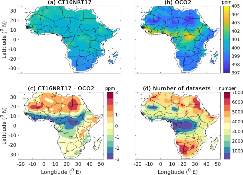
4012             A. G. Mengistu and G. Mengistu Tsidu: Comparison of CO2 from CT model and satellites over Africa

lier (2015) shows systematic error in the African savanna         Using the grid point of CT as a reference bin, the correspond-
associated with underestimating the intensity of fire during      ing GOSAT XCO2 found within a rectangle of 30 × 30 with
March at the end of the savanna burning season. Therefore,        centre at the reference bin and with a temporal mismatch of
our choice of the ACOS B3.5 Lite, hereafter GOSAT XCO2 ,          a maximum of 3 h is extracted. Moreover, CT has higher ver-
is motivated by these differences.                                tical resolutions than GOSAT. As a result, the two can not
                                                                  be directly compared. It is customary to smooth the high-
2.3    OCO-2 measurements                                         resolution data (in this case CT) with averaging kernels and
                                                                  a priori profiles of the low-resolution satellite measurements
OCO-2 is the world’s second full-time dedicated CO2 mea-          (in this case GOSAT). Besides, due to a difference between
surement satellite. It was successfully launched by the Na-       CT and GOSAT on the number of vertical levels, CT CO2
tional Aeronautics and Space Administration (NASA) on             is interpolated to vertical levels of GOSAT. The CT XCO2
2 July 2014 (Crisp et al., 2012). OCO-2 measures atmo-            (XCO2 model ) used in the comparison is computed from the
spheric carbon dioxide with the accuracy, resolution, and         interpolated CT CO2 (CO2 interp ), pressure weighting func-
coverage required to detect CO2 source and sink on a global       tion (w), XCO2 a priori (XCO2a ), column averaging kernel
and regional scale. OCO-2 has a three-band spectrometer,          of the satellite retrievals (A) and a priori profile (CO2a ) of
which measures reflected sunlight in three separate bands.        the retrievals as per the procedure discussed by Rodgers and
The O2 A-band measures molecular absorption of oxygen             Connor (2003), Connor et al. (2008), O’Dell et al. (2012),
from reflected sunlight near 0.76 µm, while the CO2 bands         Chevallier (2015), and Jing et al. (2018) and given as
are located near 1.61 and 2.06 µm (Liang et al., 2017). In
                                                                                                              interp
                                                                                             X
this study, both the nadir and glint-mode measurements of         XCO2 model = XCO2a +          wiT Ai × (CO2        − CO2a )i , (1)
OCO-2 XCO2 V7 lite level 2 covering the period from Jan-                                        i
uary 2015 to December 2016, hereafter referred to as OCO-         where i is the index of the satellite retrieval vertical level and
2 XCO2 , are used. Due to the scarcity of data, CT values         T is the matrix transpose. To compare the CT simulations
from the two releases CT2016 for the year 2015 and CT-            and the satellite observations with the flask observations, the
NRT.v2017 for the year 2016, hereafter CT16NRT17, are             vertical profiles of the satellite and CT were extracted at the
employed in this study. The OCO-2 project team at the Jet         corresponding pressure level and location within a box of
Propulsion Laboratory, California Institute of Technology,        1.50 .
produced the OCO-2 XCO2 data used in this study. The data            Correlation coefficients (R), bias and root mean square de-
can be accessed from NASA Goddard Earth Science Data              viation (RMSD) are used to assess the level of agreement be-
and Information Service Center.                                   tween the two datasets. The mean bias determines the aver-
                                                                  age deviations in XCO2 between Carbon Tracker simulation
2.4    Flask observations                                         and satellite observations. In this work the bias at the j th grid
                                                                  point is computed as
Measurements of CO2 from nine ground-based flask ob-
                                                                               n
servations near and within Africa’s land mass were ac-                      1X
cessed from the NOAA/ESRL/GMD CCGG cooperative                    Biasj =         (Si − Oi ),                                   (2)
                                                                            n i=1
air sampling network https://www.esrl.noaa.gov/gmd/ccgg/
flask.php (last access: 1 May 2019). Site description is given    where Si and Oi are CT and GOSAT XCO2 values over the
in Table 1.                                                       j th pixel at the ith time respectively. To quantify the extent
                                                                  to which XCO2 of CT and GOSAT agree, the pattern corre-
2.5    Methods                                                    lations at the j th grid point are computed as
                                                                                 1 Pn
The GOSAT and CT model XCO2 time series used in                                  n    i=1 (Si − S)(Oi − O)
                                                                  Rj = q P                     q P                   ,        (3)
this investigation span 5 years, ranging from May 2009 to                   1   n
                                                                                    (S i − S) 2 1    n
                                                                                                         (O i − O) 2
                                                                           n    i=1              n   i=1
April 2014. Atmospheric CO2 concentrations of NOAA Car-
bon Tracker have global coverage with a 30 × 20 longitude–        where S and O are the mean values of Si and Oi over the
latitude resolution which covers 426 grid boxes in our            j th pixel. The RMSD which shows the standard error of the
study area. Satellite observations, however, are different from   model with respect to the observation at the j th grid point is
model assimilation and have gaps for various reasons (e.g.        computed as
cloud and the observational mode of the satellite). As a re-                   v
                                                                               u n
sult, there is no one-to-one spatiotemporal match between                      u1 X
the two datasets. For example, CO2 products from the two          RMSDj = t            ((Si − S) − (Oi − O))2 ;              (4)
                                                                                 n i=1
datasets are not directly comparable since CT is a 3-hourly
smooth and regular grid dataset, whereas GOSAT XCO2 is            this is the centered pattern root mean squared (rms) differ-
irregularly distributed in space and time. Thus, the CT CO2       ence which is obtained from the rms error after the difference
is extracted on the time and location of GOSAT-XCO2 data.         in the mean has been removed (Taylor, 2001).

Atmos. Meas. Tech., 13, 4009–4033, 2020                                             https://doi.org/10.5194/amt-13-4009-2020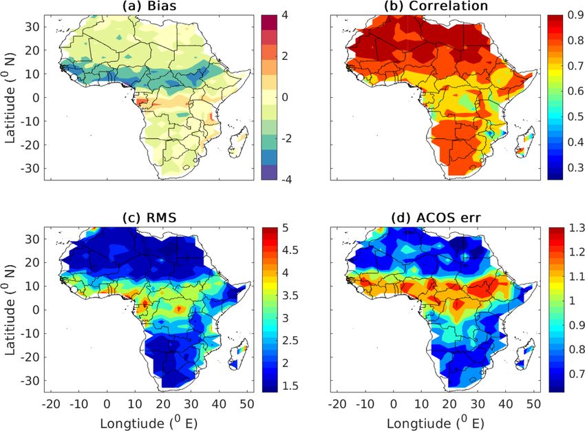
A. G. Mengistu and G. Mengistu Tsidu: Comparison of CO2 from CT model and satellites over Africa 4013
Table 1. Information on flask observation sites near and within Africa’s land mass.
Code Name Country Latitude Longitude Altitude Air pressure at
(◦ N) (◦ E) (m a.s.l.) T = 25 ◦ C (Pa)
ASC Ascension Island Ascension Island −7.967 −14.400 85.00 100 342.02
ASK Assekrem Algeria 23.262 5.632 2710.00 73 571.64
CPT Cape Point South Africa −34.352 18.489 230.00 98 682.99
IZO Izana, Canary Islands Spain 28.309 −16.499 2372.90 76 650.84
LMP Lampedusa Italy 35.520 12.620 45.00 100 803.63
MKN* Mt. Kenya Kenya −0.062 37.297 3644.00 65 579.92
NMB Gobabeb Namibia −23.580 15.030 456.00 96 141.54
SEY Mahe Island Seychelles −4.682 55.532 2.00 101 301.78
WIS Weizmann, Ketura Israel 29.965 35.060 151.00 99 584.09
∗ Indicates discontinued site or project.
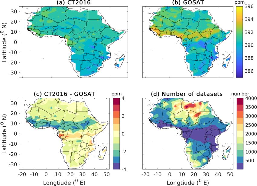
Comparison with in situ flask observation is achieved in southward of the Equator over arid environments (Williams
a way that the Carbon Tracker and satellite observations are et al., 2007). However, Fig. 1b shows that GOSAT observa-
taken at a corresponding pressure level of the in situ flask tions have some limitations in simulating this spatial pattern
observation (as mentioned in Table 1) in order to correspond in comparison to CT.
to flux towers’ surface observation. Furthermore, the datasets Figure 1c shows the mean difference (CT2016−GOSAT)
are resampled to fit the flask observations in a 30 X30 window XCO2 which ranges from −4 to 2 ppm. The highest dif-
centered on the flux towers, and the available months were ference between the CT2016 and GOSAT XCO2 (as high
averaged. as −4 ppm) is observed over the northern part of Equato-
rial Africa (e.g. southern Guinea, southern Ghana, southern
Nigeria, south-east of central Africa, western Ethiopia and
3 Results and discussions South Sudan.), which is also known for near-year-round rain-
fall and relatively dense vegetation. The regions are known
3.1 Comparison of XCO2 mean climatology from for their rainforest (Malhi et al., 2013). The likely expla-
NOAA CT2016 and GOSAT nation could be that the XCO2 mean (over 5 years) may
be slightly positively biased due to fewer GOSAT observa-
The column-averaged mole fraction of CO2 obtained from tions as shown in Fig. 1d. The satellite retrievals have noise
the NOAA Carbon Tracker model and GOSAT observation which can be smoothed out when a large number of datasets
was compared. The results are based on 426 grid boxes uni- is averaged. The strategy and methods for cloud screening in
formly distributed to cover the whole of Africa’s land region. GOSAT retrievals could lead to a smaller number of obser-
The analysis was based on 5 years of daily data starting from vations in the equatorial region (Crisp et al., 2012; O’Dell
May 2009 to April 2014. et al., 2012; Yoshida et al., 2013; Chevallier, 2015; Deng
Figure 1 shows the temporal average of CT2016 (Fig. 1a) et al., 2016b). The number of datasets used for comparison
and GOSAT (Fig. 1b) XCO2 distribution. The major com- range from 14 to 4288 from grid box to grid box, with a
mon spatial feature in the mean map of XCO2 from GOSAT spatial mean of 1109 data over the continent. Figure 1c also
and CT2016 reanalysis is dipole structure characterized by shows CT2016 simulations are overall lower than the values
high XCO2 northward of the Equator and low XCO2 south- of GOSAT observation over most regions, with exceptions
ward of the Equator, with the exception of some part of Equa- in Gabon, Congo, southern Kenya and southern Tanzania,
torial Guinea and the Republic of Congo for CT (Fig. 1a) where CT2016 simulations are higher than GOSAT observa-
and part of the Democratic Republic of Congo for GOSAT tions by more than 1 ppm. The spatial distribution of global
(Fig. 1b); these are characterized by spatially anomalous atmospheric CO2 is not uniform because of the irregularly
high XCO2 . The Southern Africa region is characterized by distributed sources of CO2 emissions, such as large power
weaker anthropogenic CO2 emission and higher CO2 uptake plant and forest fire and biospheric assimilation as clearly
by the vegetation than North Africa (Ciais et al., 2011). This noted above.
contributed to the observed dipole distribution. Another im- Figure 2a shows differences between CT2016 and GOSAT
portant pattern is the anomalous peak over the annual av- XCO2 , which ranges from −4 to 3 ppm. Out of 100 % oc-
erage location of the ITCZ (Fig. 1b) which appears to fade currence, more than 90 % of observed differences are within
over eastern Africa. This is in agreement with the fact that ±2 ppm. The mean difference between CT2016 and GOSAT
carbon stocks and net primary production per unit land area means is about −0.27 ppm, with the standard deviation of
are high over Equatorial Africa and decrease northward and 0.98 ppm indicating better regional consistency and low po-
https://doi.org/10.5194/amt-13-4009-2020 Atmos. Meas. Tech., 13, 4009–4033, 2020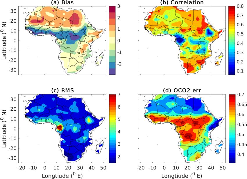
4014              A. G. Mengistu and G. Mengistu Tsidu: Comparison of CO2 from CT model and satellites over Africa

Figure 1. Distribution of 5-year averages of CT2016 (a) and GOSAT (b) XCO2 and their difference (c) gridded in 30 × 20 bins over Africa’s
Land mass; and the total number of datasets at each grid from the GOSAT observations (d).

tential outliers. Moreover, a negative mean of the difference
implies that XCO2 simulated from CT2016 is lower than that
of GOSAT retrievals over Africa’s land mass.
   Because of selection criteria which permit a difference
of 3◦ long and wide, the two datasets are not exactly at
the same point. The impact of the relative distance between
them should be assessed before performing any statistical
comparison. Figure 2b depicted the colour-coded scatter plot
of CT2016 model simulation versus GOSAT to determine
whether the discrepancy between the datasets arises from
the spatial mismatch. The colour code indicates the relative
distance between the model and observation datasets. For
these datasets the 50th percentile has a relative distance of
1.190 , which means 50 % of the data have a relative dis-
tance of shorter than 1.190 . The maximum relative distance
between them is 2.120 . However, there is no indication that           Figure 2. Histogram of the difference of CT2016 relative to
this has been the case since the scatter is not a function of          GOSAT (a) and colour code scatter diagram of XCO2 concentra-
the relative distance between the datasets. For example, data          tion as derived from CT2016 and GOSAT (b). Colour indicates the
points with blue colour with the lowest location difference            relative distance in unit of degrees as shown in the colour bar be-
are scattered everywhere instead of along the 1 : 1 line. Fur-         tween datasets.
thermore, we found the bias of −0.26 ppm, correlation co-
efficient of 0.86 and RMSD of 2.19 ppm for datasets which
have a relative distance shorter than 1.190 . On the other hand,       in this comparison are shown in Fig. 1d. As is depicted in
the bias, correlation coefficient, and RMSD are −0.33, 0.86            Fig. 3a, the bias ranges from −4 to 2 ppm with a mean bias
and 2.22 ppm for those which are above 1.190 . These statis-           of −0.28 ± 1.05 ppm (see Table 2). A larger negative bias of
tics confirm that there is no strong discrepancy due to our            about −2 ppm was found along the annual mean position of
selection criteria.                                                    the ITCZ, the main climatic mechanisms controlling rainfall
   Figure 3 shows a statistical comparison of XCO2 from the            in Africa. Systematic errors due to the ITCZ and the East
CT2016 and GOSAT over Africa. The number of data used                  African Monsoon need to be addressed well in satellite re-
                                                                       trievals and modelling works. The correlation varies from

Atmos. Meas. Tech., 13, 4009–4033, 2020                                                  https://doi.org/10.5194/amt-13-4009-2020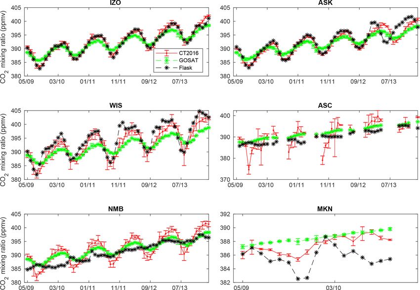
A. G. Mengistu and G. Mengistu Tsidu: Comparison of CO2 from CT model and satellites over Africa                                      4015

Figure 3. Spatial patterns of bias (a), correlation (b), RMSD (c) of the two datasets, and mean posteriori estimate of XCO2 uncertainty from
GOSAT (d).

0.4 over some isolated pockets in Congo, Tanzania, Mozam-               3.2    Comparison of monthly average time series of
bique, Uganda, and western Ethiopia to 0.9 over the northern                   NOAA CT2016 and GOSAT XCO2
part of Africa above 13◦ N, eastern Ethiopia and the Kala-
hari. Figure 3b depicts the correlation coefficient between             Figures 4–6 show monthly mean XCO2 from CT2016 and
GOSAT and Carbon Tracker XCO2 . The region with poor                    GOSAT averaged over North Africa, Equatorial Africa, and
correlation also exhibits high RMSD as shown in Fig. 3c. To             Southern Africa respectively. Figures 4a–6a depict the ex-
understand whether this discrepancy originates from model               istence of an overall very good agreement for the monthly
weakness alone or terrible satellite visibility when the ITCZ           averages with respect to amplitudes and phases of XCO2 .
is present and clouds are extremely thick and widely present,           However, XCO2 from the two datasets slightly disagree in
we have looked at the GOSAT posterior estimates of XCO2                 capturing the seasonal cycle over Southern Africa.
error (Fig. 3d), which are high over regions where the bias                Figure 4a shows that XCO2 concentration reaches maxi-
and RMSD between GOSAT and Carbon Tracker XCO2                          mum in April and minimum in September over North Africa.
is high. GOSAT’s posterior estimate of XCO2 error is a                  Consistent with this evidence, other authors (e.g. Zhou et al.,
combination of instrument noise, smoothing error and in-                2008) have indicated the presence of strong absorption of
terference error (Connor et al., 2008; O’Dell et al., 2012).            CO2 by vegetation during August in the Northern Hemi-
This posterior estimate of XCO2 error does not include for-             sphere. This is the most likely the cause of the minimum
ward model error, which may lead to underestimation of the              concentration observed during September over North Africa.
true error of satellite XCO2 by a factor of 2 (O’Dell et al.,           Both datasets show a concentration of XCO2 increases from
2012). Therefore, part of the discrepancy is clearly linked             October to April and decreases from May to September (see
to satellite retrieval uncertainty, which might have been am-           also Table 4). Moreover, the two datasets show a monthly
plified due to the small number of data points used to cal-             mean regional mean bias of −0.36 ppm with a correlation of
culate the mean error of GOSAT XCO2 measurements (see                   1.0 and a small root mean square deviation of 0.36 ppm (see
Fig. 1d). In general, the two datasets are characterized by a           Table 3).
high spatial mean correlation of 0.83 ± 1.20, a global offset              Figure 5a shows that XCO2 concentration reaches max-
of −0.28 ± 1.05 ppm, which is the average bias, a regional              ima (392.99 ppm) for CT2016 in March and (393.53 ppm)
precision of 2.30 ± 1.46 ppm, which is average RMSD, and                for GOSAT in January and minima (389.56 ppm for CT2016
a relative accuracy of 1.05 ppm, which is the standard devia-           and 389.32 ppm for GOSAT) in October over Equatorial
tion in the bias as depicted in Table 2.                                Africa. The largest monthly mean difference of −1.34 ppm
                                                                        and the smallest of −0.05 ppm between the two datasets

https://doi.org/10.5194/amt-13-4009-2020                                                   Atmos. Meas. Tech., 13, 4009–4033, 2020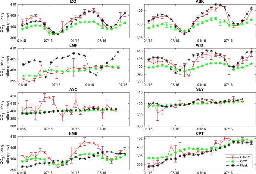
4016              A. G. Mengistu and G. Mengistu Tsidu: Comparison of CO2 from CT model and satellites over Africa

Table 2. Summary of the statistical relation between CT2016 and GOSAT observation. The statistical tools shown are the mean correlation
coefficient (R), the spatial average of bias (Bias), the spatial average root mean square deviation (RMSD), the standard deviation in bias (SD
of bias), GOSAT posteriori estimate of XCO2 error (GOSAT err), the standard deviation in CT2016 XCO2 (CT2016 SD) and the standard
deviation in GOSAT XCO2 (GOSAT SD). The number of data used in the statistics is 472 792 over 426 pixels covering the study period; the
distribution at each grid point is shown in Fig. 1d. Negative bias indicates that CT2016 XCO2 is lower than GOSAT XCO2 values.

                  Statistical tool      R       Bias     RMSD      SD of bias     GOSAT err        CT2016 SD       GOSAT SD
                                              (ppm)       (ppm)       (ppm)          (ppm)             (ppm)           (ppm)
                  Values             0.83    −0.284         2.30        1.05              0.91           0.90           1.55

Table 3. Summary of statistical relation between CT2016 and GOSAT observation. The statistical analysis was made using monthly averaged
time series of 60 months (i.e. months from May 2009 to April 2014).

                                Statistics              R      Bias (ppm)     RMSD (ppm)          Number of data
                                Africa                 0.997       −0.254         0.265              698 505
                                North Africa           0.996       −0.361         0.345              424 070
                                Equatorial Africa      0.977       −0.172         0.708              101 660
                                Southern Africa        0.964        0.006         0.841              172 775

were observed in December and in April respectively (Ta-                    example, Fig. 6b shows a positive bias from February to July
ble 4). Moreover, both datasets show that concentration of                  and negative bias from August to December over Southern
CO2 increases from October to March, while it decreases                     Africa.
from June to October. This similarity in the seasonal vari-                    Figures 4c–6c show the histogram of difference. The mean
ability of the two datasets shows that they are in good agree-              difference between CT2016 simulation and GOSAT obser-
ment in terms of amplitude and phase. In addition, the two                  vation of XCO2 is −0.36 ppm with a standard deviation of
datasets show a monthly average regional average bias of                    0.35 ppm over North Africa (see Fig. 4c); Fig. 5c presents a
−0.17 ppm, correlation of 0.98 and a small root mean square                 mean difference of −0.17 ppm with a standard deviation of
deviation of 0.71 ppm over Equatorial Africa (see Table 3).                 0.71 ppm over Equatorial Africa and Fig. 6c reveals a mean
Figure 6a shows maximum XCO2 concentration in April                         difference of 0.01 ppm and a standard deviation of 0.85 ppm,
(391.04 ppm) for CT2016 and in October (391.28 ppm) for                     which indicates that XCO2 from CT2016 was slightly higher
GOSAT and minimum in May (389.30 ppm) for CT2016 and                        than that of GOSAT over Southern Africa on average. In
(388.46 ppm) for GOSAT over Southern Africa. The largest                    addition, the low standard deviation of monthly mean dif-
monthly mean difference of 1.53 and 0.03 ppm between the                    ference over North Africa typically indicates good regional
two datasets is observed in April and in July (Table 4) respec-             consistency between CT2016 and GOSAT. This is mainly
tively. Both datasets show a concentration of CO2 increases                 because North Africa is dominated by the Sahara, which is
from May to July, while it decreases from October to Novem-                 a vegetation-free area, and the systematic bias due to the
ber. However, the XCO2 from CT2016 shows a gradually                        local atmosphere–biosphere interaction is minimum. How-
increasing trend from January to April. Conversely, GOSAT                   ever, the spatial mean of monthly mean bias is slightly higher
XCO2 shows decreasing values. This is most likely the result                (−0.36 ppm) over North Africa than over Equatorial Africa
of the fact that CT2016 simulation is more sensitive to the                 (−0.17 ppm) and Southern Africa (0.01 ppm). This is possi-
growing size of the sink following the rainy season. More-                  bly due to the presence of strong local emissions from Egypt,
over, the two datasets show a monthly mean regional mean                    Algeria and Libya as well as due to long-range transport
bias of 0.07 ppm, correlation of 0.97 and RMSD of 0.87 ppm                  from the Northern Hemisphere as reported in other studies
over Southern Africa (see Table 3).                                         (Williams et al., 2007; Carré et al., 2010).
   Figures 4b–6b show regional averaged bias in the monthly                    Figures 4d–6d display the annual growth rate of XCO2 ,
mean XCO2 from CT2016 and GOSAT. Figure 4b shows                            which ranges from 1.5 to 2.7 ppm yr−1 . Moreover, the two
the presence of seasonally varying negative bias over North                 datasets are consistent in determining the annual growth
Africa. A high (< −0.5 ppm) negative bias in dry seasons                    rate. The results are found to be in good agreement with
(April to June) and low (= − 0.1 ppm) negative bias in wet                  the observed variability in the global annual growth rate
seasons (August to September) are observed. Moreover, the                   from surface measurements (http://www.esrl.noaa.gov/gmd/
strength of the bias increases from February to June. Con-                  ccgg/trends/global.html, last access: 20 March 2018) which
versely, the bias decreases from June to September. Simi-                   is 1.67, 2.39, 1.70, 2.40, and 2.51 ppm yr−1 globally dur-
larly, Figs. 5b and 6b show seasonally fluctuating bias. For                ing 2009–2013 respectively and 1.89, 2.42, 1.86,2.63, and

Atmos. Meas. Tech., 13, 4009–4033, 2020                                                          https://doi.org/10.5194/amt-13-4009-2020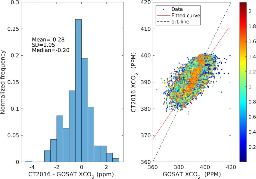
A. G. Mengistu and G. Mengistu Tsidu: Comparison of CO2 from CT model and satellites over Africa                                  4017

Figure 4. The monthly mean time series of CT2016 and GOSAT from May 2009 to April 2014 averaged over North Africa (a), bias associated
with the monthly means (b), the histogram of difference (c) and the annual growth rate obtained by subtracting the mean from the mean of
the next year (d). The error bars in (a) show the GOSAT a posteriori XCO2 uncertainty.

Figure 5. The same as Fig. 4 but over Equatorial Africa.

https://doi.org/10.5194/amt-13-4009-2020                                                 Atmos. Meas. Tech., 13, 4009–4033, 2020
4018              A. G. Mengistu and G. Mengistu Tsidu: Comparison of CO2 from CT model and satellites over Africa

Figure 6. The same as Fig. 4 but over Southern Africa.

Table 4. Five-year monthly averaged XCO2 concentration in ppm obtained from CT2016 (CT) and GOSAT (GO) and their difference
CT−GO (D) in ppm over Africa (A), North Africa (NA), Equatorial Africa (EA) and Southern Africa (SA).

  Month          A CT      A GO       AD      NA CT      NA GO    NA D     EA CT    EA GO    EA D    SA CT    SA GO    SA D
  January       391.81    392.17    −0.36     392.43     392.61   −0.18    392.22   393.53   −1.31   390.28   390.49   −0.21
  February      392.48    392.58     −0.1     393.27      393.5   −0.23    392.72   393.21   −0.49   390.52   390.06    0.46
  March         393.25    393.28    −0.03     394.02     394.29   −0.27    392.99   393.19    −0.2   390.82   389.81    1.01
  April         393.81    393.91     −0.1     394.79     395.35   −0.56    392.87   392.92   −0.05   391.04   389.51    1.53
  May           391.65    391.85    −0.21     392.92     393.73   −0.81    390.47   389.93    0.54    389.3   388.46    0.84
  June          391.49    391.94    −0.45     392.43     393.33    −0.9    391.12   390.89    0.23   389.95   389.85    0.11
  July          390.92     391.1    −0.18     391.09      391.5   −0.41    391.44   391.03    0.41   390.43    390.4    0.03
  August        389.89    389.96    −0.07      389.4     389.44   −0.04    390.92   390.72    0.21   390.37   390.61   −0.25
  September     389.26     389.4    −0.14     388.65     388.75    −0.1    390.02   389.67    0.35   390.39   391.01   −0.61
  October       389.19    389.71    −0.51     388.85     389.26   −0.41    389.56   389.32    0.24   389.95   391.28   −1.32
  November      389.97    390.43    −0.46     390.06     390.32   −0.26    389.86   390.52   −0.66    389.8   390.76   −0.96
  December      391.09    391.53    −0.45     391.42      391.6   −0.18    391.23   392.57   −1.34   389.98   390.52   −0.54

2.06 ppm yr−1 for Mauna Loa during 2009–2013 respec-                 3.3   Comparison of seasonal climatology
tively, with error bars of 0.05–0.09 ppm yr−1 for global
datasets and 0.11 ppm yr−1 for Mauna Loa datasets (Kulawik
et al., 2016). The growth rate may not be conclusive due             The seasonal cycle has important implications for flux
to the short length of the datasets used. However, it reflects       estimates (Keppel-Aleks et al., 2012). It is important to
how the CT and GOSAT observations perform with respect               analyse whether there are seasonally dependent biases
to each other.                                                       that are affecting the seasonal cycle and whether the
                                                                     datasets are capturing the same seasonal cycle. The four
                                                                     seasons considered here are December/January/February
                                                                     (DJF), March/April/May (MAM), June/July/August (JJA),
                                                                     and September/October/November (SON). DJF corresponds

Atmos. Meas. Tech., 13, 4009–4033, 2020                                              https://doi.org/10.5194/amt-13-4009-2020
A. G. Mengistu and G. Mengistu Tsidu: Comparison of CO2 from CT model and satellites over Africa 4019 Figure 7. Seasonal climatology of XCO2 for NOAA CT2016 (left panels) and GOSAT (middle panels) and their difference (right panels). to northern winter/southern summer, MAM to northern ancy between the CT2016 and GOSAT becomes significant spring/southern autumn, JJA to northern summer/southern when vegetation cover is weak during DJF and MAM (dry winter, and SON to northern autumn/southern spring respec- seasons) over North Africa. tively. Figure 7 shows the seasonal distributions of CT2016 During SON the seasonal difference in most of Africa’s (left panels) and GOSAT (middle panels) XCO2 and their land region ranges from −2 to 1 ppm. The result implies difference (CT2016−GOSAT, right panels). The distribution that CT2016 simulates lower values of XCO2 than that of clearly shows that XCO2 concentration is maximum dur- GOSAT observation, indicating that there is a better spatial ing MAM and minimum during SON over the North Africa. consistency during this season. Furthermore, during these On the other hand, maxima are found during SON and min- seasons both North and Southern Africa have a moderate ima during DJF over Southern Africa. These features are in vegetation cover following their respective summer seasons. good agreement with the rainfall climatology of the Northern The two datasets show lower regional variation (i.e. only Hemisphere and Southern Hemisphere. Moreover, Table 5 from −2 to 2 ppm) over most of Africa’s land mass. How- shows seasonally varying biases. Seasonal biases affect the ever, Equatorial Africa exhibits a mean difference lower than seasonal cycle and amplitudes, which are important for bio- −2 ppm during DJF and MAM. This indicates that the model spheric flux attribution (Lindqvist et al., 2015). tends to simulate lower than GOSAT XCO2 over the re- The right panels in Fig. 7 show that the seasonal mean dif- gion. Figure 7 (right panels) reveals XCO2 from CT2016 is ference (CT2016−GOSAT) ranges from −4 to 6 ppm, with lower than GOSAT XCO2 over North Africa. The underes- a maximum difference of 6 ppm over the Gulf of Guinea timation of observed XCO2 by the NOAA CT2016 model and Congo during JJA. However, such a maximum differ- is likely related to the skill of driving ERA-Interim data as ence was also observed over Southern Africa during DJF. noted from previous studies. For example, Mengistu Tsidu A minimum of −4 ppm over the annual mean ITCZ region (2012) has shown that the ERA-Interim data have a wet bias was observed during DJF and MAM. Moreover, the differ- over Ethiopian highlands. Mengistu Tsidu et al. (2015) have ence is above 1 ppm over Southern Africa during DJF and also shown that ERA-Interim precipitable water is higher MAM (wet season of the region). This implies high spatial than measurements from radio-sonde, FTIR and GPS obser- variability of the seasonal mean difference during different vations. Therefore, such wet bias in the driving ERA-Interim seasons (see also Table 5). It also suggests that the discrep- global circulation model (GCM) might have forced NOAA https://doi.org/10.5194/amt-13-4009-2020 Atmos. Meas. Tech., 13, 4009–4033, 2020
4020              A. G. Mengistu and G. Mengistu Tsidu: Comparison of CO2 from CT model and satellites over Africa

Figure 8. Histogram of difference for the seasonal XCO2 climatology for the DJF (a), MAM (b), JJA (c) and SON (d) seasons.

Table 5. Summary of statistical relation between CT2016 and GOSAT XCO2 : bias, correlation (R), root mean square deviation (RMSD),
standard deviation of XCO2 from CT2016 simulation (CT2016 SD), standard deviation of XCO2 from GOSAT observation (GOSAT SD),
aggregate number of coincident observations (number of data) and number of grids over the region (grid). Negative bias means CT2016 is
lower than GOSAT. The statistics are on the basis of spatial averages of seasonal averages of bias, correlation, RMSD and standard deviations.

  Region        Statistics   Bias (ppm)       R    RMSD (ppm)        CT2016 SD (ppm)       SD in GOSAT (ppm)        number of data     grid
  Africa        DJF                0.06    0.73              1.91                  1.15                     2.57           135 865     409
                MAM                0.04    0.92              1.62                  1.98                     3.25            95 942     410
                JJA                0.22    0.65              1.59                  1.12                     2.08           116 360     400
                SON               −0.37    0.76                 1                  0.94                     1.52           124 233     408
  North         DJF               −0.25    0.36              1.08                  0.67                     1.12           103 913     204
  Africa        MAM               −0.72    0.44              1.11                  0.62                     1.24            65 115     204
                JJA               −0.42    0.73              1.17                   0.9                     1.66            60 854     204
                SON               −0.35    0.66              0.53                  0.52                     0.71            91 778     204
  Equatorial    DJF               −0.52    0.68              2.47                  1.06                     3.07             22 639    121
  Africa        MAM                0.18     0.9              1.88                  1.94                     3.46              8300     115
                JJA                1.51    0.59              2.02                  1.46                     2.52             12 714    104
                SON                0.25     0.7               1.3                  1.16                     1.83             10 213    113
  Southern      DJF                1.61    0.42              1.72                  0.88                      1.9              9313      84
  Africa        MAM                1.56    0.67              0.97                  0.82                     1.31             22 527     91
                JJA                0.18    0.81              0.78                  0.93                     1.31             42 792     92
                SON               −1.16    0.77              0.81                  0.84                     1.26             22 242     91

CT2016 to generate dense vegetation which serves as a CO2                of XCO2 (−0.37 ppm) occurs during SON and the lowest
sink.                                                                    (0.04 ppm) occurs during MAM. Table 5 presents the sum-
   Figure 8 shows the mean difference between CT2016 and                 mary of statistical values for the spatial mean of each season
GOSAT XCO2 seasonal means which ranges from −0.37 to                     means. The comparison between the two datasets also shows
0.04 ppm with a standard deviation within a range of 1.00                there is a strong correlation (> 0.5) during each season over
to 1.91 ppm over the continent. The highest mean difference              the continent. However, there are moderate correlations (0.3

Atmos. Meas. Tech., 13, 4009–4033, 2020                                                     https://doi.org/10.5194/amt-13-4009-2020
A. G. Mengistu and G. Mengistu Tsidu: Comparison of CO2 from CT model and satellites over Africa 4021
Figure 9. CO2 time series for the coincident period for CT2016 (red), GOSAT (green) and flask (black). The standard deviation in computing
the monthly mean is indicated by the vertical error bar.
to 0.5) during DJF and MAM over North Africa and during riorated over sites in Equatorial Africa (ASC and MKN) and
DJF over Southern Africa. The low correlation over North Southern Africa (MNB). Over MKN, CT2016 shows better
Africa may be linked to a weak absorption by vegetation correlation (0.43) than GOSAT observation (0.08). In addi-
and a strong emission from human activities during winter tion, monthly amplitudes from CT2016 were closer to the
as reported elsewhere (Liu et al., 2009; Kong et al., 2010). flask observations, suggesting that satellite retrievals need
Moreover, Table 5 shows that the seasonal biases are neg- much attention over the region. On the other hand, GOSAT
ative over North Africa, while they are mostly positive over observations were found to be in better agreement with flask
Equatorial and Southern Africa. Negative biases are observed observations over ASC. Zhang et al. (2015) also show that
during DJF and SON over Equatorial and Southern Africa re- GOSAT data were correlated well with ground observation
spectively, implying that XCO2 from CT2016 are lower than and found to be more centralized, having high system stabil-
from GOSAT during dry seasons. ity, especially over the ocean.
CT2016 has a better sensitivity over IZO, ASK and NMB.
3.4 Comparison of GOSAT and CT2016 with flask Moreover, CT2016 compared better with flask observations
observations than GOSAT over these sites; almost all flask observations
are within the standard deviations of the monthly mean of
Comparison of GOSAT and CT2016 with flask observation CT2016. However, GOSAT observations were found to be in
is carried out over six available ground-based flask observa- better agreement with flask observations than CT2016 was
tions. For the comparison, the volume mixing ratio of CO2 over WIS and ASC. On the other hand, both CT2016 and
from GOSAT and CT2016 at the pressure level that corre- GOSAT have low sensitivity to flask observation over MKN
sponds to surface flask observations (see Table 1) was con- (see Fig. 10). Similar to our previous discussion on sites in
sidered. North Africa (IZO, ASK and WIS), CT2016 underestimates
Monthly mean CO2 from flask observations at IZO and XCO2 during August, September, and October (wet season)
ASK in North Africa shows an excellent agreement with both compered to GOSAT observation and overestimates XCO2
CT2016 and GOSAT CO2 . Moreover, CT2016 has a better during January to June. However, the CT2016 and the flask
sensitivity in capturing the amplitudes than GOSAT, where observations exhibit better agreement, indicating a bias in
observations from GOSAT mostly underestimate higher val- GOSAT observation during the wet season.
ues of flask CO2 (Fig. 9). However, this agreement has dete-
https://doi.org/10.5194/amt-13-4009-2020 Atmos. Meas. Tech., 13, 4009–4033, 20204022 A. G. Mengistu and G. Mengistu Tsidu: Comparison of CO2 from CT model and satellites over Africa
Table 6. Summary of statistical relations of CT2016 and GOSAT observation with respect to flask observations. The statistical analysis was
made using monthly averages covering the period from May 2009 to April 2014).
Code CT R GOSAT R CT bias GOSAT bias CT RMSD GOSAT RMSD number of data
(ppm) (ppm) (ppm) (ppm)
ASC 0.58 0.93 1.05 1.84 4.46 1.07 39
ASK 0.90 0.90 −0.63 −0.76 1.97 2.23 60
NMB 0.75 0.91 1.40 1.13 3.12 1.56 60
IZO 0.99 0.97 0.24 −0.36 0.70 1.40 60
MKN 0.40 0.04 1.83 2.88 1.48 1.64 17
WIS 0.93 0.83 −1.57 −2.61 1.95 3.31 60
Figure 10. De-trended seasonal cycle of XCO2 during 2009–2014 from CT2016 (red), GOSAT (green) and flask (black) observations. The
standard deviation of the monthly variables is indicated by error bars.
3.5 Comparison of mean XCO2 from NOAA (> 400 ppm) XCO2 values over North Africa, while these
CT16NRT17 and OCO-2 high XCO2 values are observed over Equatorial Africa in the
case of OCO-2 observation. The two datasets show a dis-
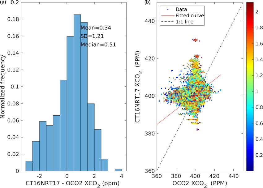
The strong El Niño event that occurred during 2015–2016 crepancy over Equatorial Africa, where CT16NRT17 simu-
provides an opportunity to compare the performance of lates low XCO2 values (< 401 ppm), while OCO-2 observes
CT16NRT17 during strong El Niño events. Because of the high values of XCO2 (> 401 ppm). Both datasets show
decline in terrestrial productivity and enhancement of soil moderate XCO2 values which range from 397 to 400 ppm
respiration, the concentration of CO2 increases during El over Southern Africa. The XCO2 distribution from OCO-
Niño events (Jones et al., 2001). In this section we compare 2 is consistent with the maximum CO2 concentration re-
mean XCO2 of NOAA CT16NRT17 and NASA’s OCO-2 ported in a past study by Williams et al. (2007), implying
covering the period from January 2015 to December 2016. that the CT16NRT17 likely underestimates XCO2 values
The comparison was made based on the selection crite- over Equatorial Africa. It is also possible that the discrep-
ria discussed in Sect. 2.5. Figure 11 shows the mean distri- ancy is a compounded effect of OCO-2 XCO2 positive bias
bution of XCO2 from CT16NRT17 (Fig. 11a) and OCO-2 over the region (O’Dell et al., 2012; Chevallier, 2015). Fig-
(Fig. 11b) over Africa’s land mass. CT16NRT17 shows high
Atmos. Meas. Tech., 13, 4009–4033, 2020 https://doi.org/10.5194/amt-13-4009-2020A. G. Mengistu and G. Mengistu Tsidu: Comparison of CO2 from CT model and satellites over Africa 4023 Figure 11. Distribution of 2-year average XCO2 of CT16NRT17 (a) and OCO-2 (b) XCO2 and their difference (c) gridded in 30 × 20 bins; and (d) the total number of datasets at each grid. ure 11c shows the mean difference between the 2-year mean of XCO2 from CT16NRT17 and OCO-2, which is in the range from −2 to 2 ppm. However, high (< −2 ppm) neg- ative mean difference between the two datasets over rain- forest regions (Gulf of Guinea and Congo basin) and the ITCZ over eastern Africa (South Sudan and south-eastern Sudan) is observed, implying that CT16NRT17 simulates lower XCO2 values than that of OCO-2 observation over regions where vegetation uptake is strong. Conversely, high (> 1) positive mean difference over the Sahara, Somalia and Tanzania implies CT16NRT17 simulates higher XCO2 val- ues than OCO-2 observation where the vegetation uptake is weak. Moreover, a positive (> 2) mean difference over Egypt, Libya, Sudan, Chad, Niger, Mali and Mauritania is likely due to overestimates of XCO2 emission from local sources by CT16NRT17. Overall, the two datasets show a Figure 12. Histogram of the difference of CT16NRT17 relative to fairly reasonable agreement with a correlation of 0.60 and an OCO-2 (a) and colour code scatter diagram of XCO2 concentra- offset of 0.36 ppm, a regional precision of 2.51 ppm and a tion as derived from CT16NRT17 and OCO-2 (b). Colour indicates regional accuracy of 1.21 ppm. the relative distance in unit of degrees as shown in the colour bar Figure 12a shows the histogram of 2-year mean differ- between datasets. ence, which is characterized by a positive mean of 0.34 ppm and a standard deviation of 1.21 ppm. This suggests that CT16NRT17 simulates high XCO2 as compared to observa- distance. The random scatter of blue dots implies that the sta- tions from OCO-2 over Africa’s land mass. tistical discrepancies do not arise from the relative distance Because of the presence of spatial and temporal mismatch between the two datasets. More specifically, a statistical com- of some level between CT16NRT17 and OCO-2 datasets, it is parison of datasets lower and higher than the 50th percentile important to assess the effect of relative distance between the (1.20 ) shows bias of 0.58 and 0.57 ppm, correlation of 0.57 datasets. Figure 12b shows a colour-coded distribution of the and 0.57 and RMSD of 2.65 and 2.67 ppm respectively. two datasets. In the figure colour codes indicate the relative https://doi.org/10.5194/amt-13-4009-2020 Atmos. Meas. Tech., 13, 4009–4033, 2020
4024              A. G. Mengistu and G. Mengistu Tsidu: Comparison of CO2 from CT model and satellites over Africa

Table 7. Summary of the statistical relation between CT16NRT17 and OCO-2 observation. The statistical tools shown are the mean correla-
tion coefficient (R), the average of bias (Bias), the average root mean square deviation (RMSD), the standard deviation in bias (SD of bias),
mean posteriori estimate of XCO2 error from OCO-2 (OCO-2 err), the standard deviation in CT16NRT17 XCO2 (CT16NRT17 SD) and the
standard deviation in OCO-2 XCO2 (OCO-2 SD). Positive bias indicates that CT16NRT17 is higher than OCO-2. The number of data used
in the statistics is 1 659 411 over 426 pixels covering the study period; the distribution at each grid point is shown in Fig. 11d.

                  Statistical tool      R     Bias     RMSD        SD of bias   OCO-2 err   CT16NRT17 SD       OCO-2 SD
                                            (ppm)       (ppm)         (ppm)        (ppm)           (ppm)          (ppm)
                  Values             0.6     0.34           2.57        1.21         0.55               0.55          1.28

Figure 13. The bias (a), correlation (b), RMSD (c) of model and OCO-2 XCO2 and mean posteriori estimate of XCO2 error from OCO-2 (d).

Table 8. Annual growth rate (AGR) of XCO2 over Africa’s land                0.8 over Africa’s land mass. Good correlations of above 0.6
mass from CT16NRT17 and OCO-2. The results are obtained as                  are seen over many regions of the continent, while weak cor-
the mean annual difference of 2015 and 2016 values.                         relation of less than 0.2 and higher root mean square error
                                                                            (> 3 ppm) are observed over small pockets of the Equatorial
       Region                AGR of CT      AGR Of OCO-2                    and eastern Africa regions (see Fig. 13c). These regions also
                             (ppm yr−1 )     (ppm yr−1 )                    show a higher (> 0.65 ppm) error in satellite retrieval (see
       North Africa              3.10                3.33                   Fig. 13d). In addition, Fig. 11d shows the number of obser-
       Equatorial Africa         3.14                3.42                   vations are small (< 1000) over these regions. This may con-
       Southern Africa           3.20                3.16                   tribute to the observed discrepancy over these regions. How-
                                                                            ever, weak correlations are also observed over a wider area
                                                                            in North Africa such as Mauritania, Mali, Algeria and some
                                                                            regions of Niger, where satellite errors are low and sufficient
   Figure 13 shows the comparison of mean XCO2 from                         data are obtained. Poor correlation and higher RMSD values
CT16NRT17 and OCO-2 covering the period from Jan-                           are observed over south-western Ethiopia.
uary 2015 to December 2016. The number of data used are
displayed in Fig. 11d. Figure 13a depicts the bias which                    3.6   Comparison of monthly average time series of
ranges from −2 to 2 ppm with a mean bias of 0.34 ppm. How-                        NOAA CT16NRT17 and OCO-2 XCO2
ever, higher biases (< −2 ppm) are observed over Equatorial
Africa along the annual average location of the ITCZ. Fig-                  Figures14–16 show a 2-year monthly average time series
ure 13b shows the correlation map with values from 0.2 to                   comparison of XCO2 from CT16NRT17 and OCO-2 over

Atmos. Meas. Tech., 13, 4009–4033, 2020                                                      https://doi.org/10.5194/amt-13-4009-2020
You can also read