Extreme wet seasons - their definition and relationship with synoptic-scale weather systems - WCD
←
→
Page content transcription
If your browser does not render page correctly, please read the page content below
Weather Clim. Dynam., 2, 71–88, 2021
https://doi.org/10.5194/wcd-2-71-2021
© Author(s) 2021. This work is distributed under
the Creative Commons Attribution 4.0 License.

Extreme wet seasons – their definition and relationship
with synoptic-scale weather systems
Emmanouil Flaounas, Matthias Röthlisberger, Maxi Boettcher, Michael Sprenger, and Heini Wernli
Institute for Atmospheric and Climate Science, ETH Zurich, Zurich, Switzerland

Correspondence: Emmanouil Flaounas (emmanouil.flaounas@env.ethz.ch)

Received: 30 June 2020 – Discussion started: 8 July 2020
Revised: 24 December 2020 – Accepted: 13 January 2021 – Published: 1 February 2021

Abstract. An extreme aggregation of precipitation on the           But interlatitudinal influences are also shown to be impor-
seasonal timescale, leading to a so-called extreme wet sea-        tant: tropical moisture exports, i.e., the poleward transport
son, can have substantial environmental and socio-economic         of tropical moisture, can contribute to extreme wet seasons
impacts. This study has a twofold aim: first to identify and       in the midlatitudes, while breaking Rossby waves, i.e., the
statistically characterize extreme wet seasons around the          equatorward intrusion of stratospheric air, may decisively
globe and second to elucidate their relationship with specific     contribute to the formation of extreme wet seasons in the
weather systems.                                                   tropics. Three illustrative examples provide insight into the
    Extreme wet seasons are defined independently at every         synergetic effects of the four identified weather systems on
grid point of ERA-Interim reanalyses as the consecutive 90 d       the formation of extreme wet seasons in the midlatitudes, the
period with the highest accumulated precipitation in the 40-       Arctic and the (sub)tropics.
year period of 1979–2018. In most continental regions, the
extreme seasons occur during the warm months of the year,
especially in the midlatitudes. Nevertheless, colder periods
might be also relevant, especially in coastal areas. All iden-     1   Introduction
tified extreme seasons are statistically characterized in terms
of climatological anomalies of the number of wet days and          This study focuses on extreme precipitation, albeit not on
of daily extreme events. Results show that daily extremes are      short timescales of single weather systems like thunder-
decisive for the occurrence of extreme wet seasons in regions      storms or cyclones, but on the seasonal timescale. The anal-
of frequent precipitation, e.g., in the tropics. This is in con-   ysis of extreme precipitation events on timescales of hours
trast to arid regions where wet seasons may occur only due to      to a few days has long been a centerpiece of weather and
anomalously frequent wet days. In the subtropics and more          climate research due to their relevance for a variety of socio-
precisely within the transitional zones between arid areas and     economic aspects including damages to infrastructures and
regions of frequent precipitation, both an anomalously high        loss of life. Indeed, many studies investigated single ex-
occurrence of daily extremes and of wet days are related to        treme precipitation events to identify the key dynamical and
the formation of extreme wet seasons.                              physical processes involved (e.g., Doswell et al., 1998; Mas-
    A novel method is introduced to define the spatial ex-         sacand et al., 1998; Delrieu et al., 2005; Holloway et al.,
tent of regions affected by a particular extreme wet season        2012; Moore et al., 2012; Winschall et al., 2012; Flaounas
and to relate extreme seasons to four objectively identified       et al., 2016). In addition, climatological studies quantified
synoptic-scale weather systems, which are known to be as-          the relationship of extreme precipitation events with specific
sociated with intense precipitation: cyclones, warm conveyor       synoptic-scale flow systems like cyclones (Pfahl and Wernli,
belts, tropical moisture exports and breaking Rossby waves.        2012), fronts (Catto and Pfahl, 2013) and warm conveyor
Cyclones and warm conveyor belts contribute particularly           belts (Pfahl et al., 2014). Finally, another important strand
strongly to extreme wet seasons in most regions of the globe.      of research addressed the future evolution of extreme precip-
                                                                   itation events in a changing climate, using a plethora of sim-

Published by Copernicus Publications on behalf of the European Geosciences Union.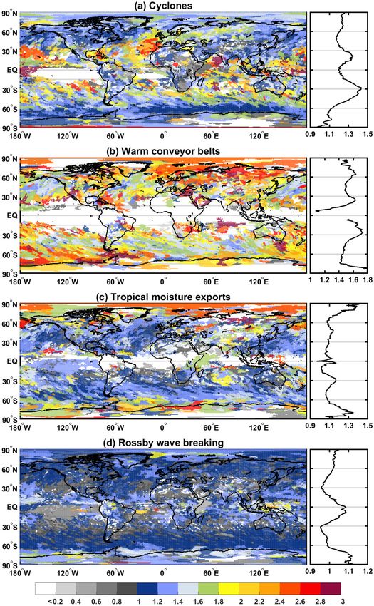
72       E. Flaounas et al.: Extreme wet seasons – their definition and relationship with synoptic-scale weather systems

ulation ensembles, reanalysis datasets and observations (e.g.,     unique and recurrent weather system, such as tropical cy-
Easterling et al., 2000; Shongwe et al., 2011; Pfahl et al.,       clones, or they may be related to a variety of weather sys-
2017). However, socio-economic impacts related to precipi-         tems that occur sequentially in the considered season, fa-
tation are not limited to the occurrence of single, outstanding    vored by regional- or global-scale atmospheric conditions.
extreme precipitation events, but they are also potentially re-    For instance, Davies (2015) and Röthlisberger et al. (2019)
lated to accumulated precipitation on longer timescales. For       showed that the anomalously wet and stormy European win-
instance, the costliest, hyperactive North Atlantic hurricane      ter of 2013–2014 was related to recurrent upper-tropospheric
season of 2017 had a significant impact on the coastal pop-        flow conditions that triggered a succession of high-impact
ulation of the US due to an anomalous sequence of tropical         weather systems. Priestley et al. (2017) showed that this was
cyclones that made landfall, causing damages of the order          due to anomalous Rossby wave activity leading to cyclone
of USD 370 billion and loss of human life (Halverson, 2018;        clustering that affected in the UK in particular with a fre-
Taillie et al., 2020). The 2017 hurricane season did not in-       quency of about 2.5 cyclones per day. Climatological influ-
clude any record-breaking intense hurricanes, although it in-      ences might be also important for seasonal precipitation, for
cluded several hurricanes producing extreme precipitation.         instance in the Mediterranean. A large majority of precipita-
Another example of seasonal-scale environmental risk is the        tion in this region is due to intense cyclones (Flaounas et al.,
direct relationship between the seasonal rainfall over the Sa-     2018); however, the intensity of cyclones and related rain-
hel and the epidemics of meningitis (Sultan et al., 2005). In      fall is influenced by the North Atlantic Oscillation and the
fact, an anomalously wet African monsoon season may have           El Niño–Southern Oscillation (Mariotti et al., 2002; Raible,
a detrimental impact on public health on continental scales        2007). Seasonal precipitation has been the theme of numer-
(Polcher et al., 2011).                                            ous studies in the past; however, in this study we add to the
   The factors contributing to the formation of extreme sea-       scientific understanding of this topic by focusing on extreme
sons may not be linked directly to the anomalous occurrence        wet seasons and performing a systematic analysis of how in-
of extreme events as intuitively expected. Röthlisberger et        dividual weather systems contribute to their occurrence.
al. (2020) showed that an extreme hot or cold season may not          Weather systems on different spatial scales may interact to
be always provoked by the repetitive occurrence of excep-          give rise to extreme wet seasons. For instance, synoptic-scale
tionally high or low temperatures, respectively. In contrast,      atmospheric conditions may favor the occurrence of and in-
an extremely warm summer can also occur due to its coldest         tensify mesoscale weather systems, which in turn may lead to
days being anomalously mild. Therefore, the seasonal distri-       variable amounts of precipitation depending on their physical
bution of weather variables plays an important role in char-       characteristics, e.g., water vapor content, precipitation effi-
acterizing a season. Despite their high socio-economic rel-        ciency. It is a scientific challenge to delineate and objectively
evance, the analysis of extreme wet seasons has not gained         identify all links in the chain of events governing precipita-
high visibility in climate research so far. This study addresses   tion in climatological datasets. As mentioned above, several
this research gap and aims to contribute to a better under-        studies have quantified the role of specific weather systems
standing of the characteristics of extreme wet seasons around      such as cyclones (Hawcroft et al., 2012; Pfahl and Wernli,
the globe and to provide insight into the responsible weather      2012; Flaounas et al., 2016), fronts (Catto et al., 2012), warm
systems.                                                           conveyor belts (Pfahl et al., 2014), tropical moisture exports
   The definition and identification of distinct precipitation     (Knippertz and Wernli, 2010), troughs, cutoff systems and
seasons is a delicate issue and highly dependent on the re-        breaking Rossby waves (e.g., Martius et al., 2006; de Vries
gion of interest. Monsoon-affected regions typically experi-       et al., 2018; Moore et al., 2019; De Vries, 2020) for precip-
ence a clear onset date that signals the beginning of the pre-     itation on regional and global scales. Nevertheless, it is an
cipitation period (Bombardi et al., 2017, 2019), while several     open question whether these weather systems occur succes-
midlatitude areas experience more than one rainy season, or        sively or act synergistically to form an extreme wet season in
they are characterized by wet conditions year-round. On the        a certain region. Moreover, it is an open question whether ex-
other hand, semi-arid and arid areas do not have clearly pre-      treme wet seasons may be produced by more frequent daily
ferred precipitation periods due to the scarcity of wet days,      extreme events, more intense daily extremes, or by higher
and thus the definition of a precipitation season becomes less     persistence of moderate rainfall – or a combination of these
meaningful in these areas (Wu et al., 2007). Regardless, if        options. In fact, the aggregated contribution of a weather sys-
a region experiences an extreme seasonal accumulation of           tem to seasonal precipitation may be statistically character-
precipitation, e.g., due to an anomalous frequency of daily        ized by the frequency and intensity of the precipitation it pro-
extreme events, this has a potentially hazardous effect. In-       duces (e.g., Toreti et al., 2010; Moon et al., 2019). This study
deed, the above examples about hurricane and monsoon sea-          uses these concepts to statistically characterize extreme wet
sons illustrate that significant seasonal precipitation anoma-     seasons, to address their spatial coherence, and to quantify
lies may be related to both an anomalous frequency and in-         the contributions of specific weather systems. In this way,
tensity of precipitation events. Depending on the region, sea-     we aim to provide novel insight into the relationship between
sonal precipitation extremes may be related to a well-defined,

Weather Clim. Dynam., 2, 71–88, 2021                                                    https://doi.org/10.5194/wcd-2-71-2021
E. Flaounas et al.: Extreme wet seasons – their definition and relationship with synoptic-scale weather systems                  73

the statistical characteristics of extreme wet seasons and their   tation. Therefore, secondary extreme seasons have been also
dynamical origin.                                                  considered at every grid point even if these seasons may not
   In the next section, we present the datasets and methods        be statistically considered as extreme. They correspond to
used to define extreme wet seasons and to objectively iden-        90 d periods with accumulated precipitation exceeding 90 %
tify the contributing weather systems. In Sect. 3, we perform      of the precipitation in the primary extreme season at the same
a statistical approach at every grid point to characterize ex-     grid point. All primary and secondary extreme seasons at one
treme wet seasons by the number of daily extreme precip-           grid point were forced to not overlap in time. The result of
itation events and by the number of wet days that occur in         this first step is, for every grid point, a list with the primary
this season. The spatial coherence of extreme wet seasons is       extreme season and a number of secondary extreme seasons
then analyzed in Sect. 4. Section 5 shows examples of the          (zero to 28 with a median of 2). Each of these seasons is char-
complexity of how different weather systems contribute to          acterized by their time period and precipitation amount. All
extreme wet seasons, and Sect. 6 provides a global overview        results in Sect. 3 are based on this dataset.
of these contributions. Finally, Sect. 7 provides the summary
and conclusions.                                                   2.2   Spatial and temporal coherence of extreme wet
                                                                         seasons

2     Dataset and methods                                          After identifying primary and secondary extreme seasons at
                                                                   every grid point, we examine their spatial coherence. To this
2.1    Identification of extreme wet seasons                       end, we consider that two neighboring grid points are ex-
                                                                   periencing the same extreme season if their corresponding
We use daily accumulated precipitation fields from the             90 d periods overlap temporally by at least 75 %, i.e., if they
ERA-Interim (ERAI) reanalysis of the European Centre for           have at least 68 d in common. Figure 1 illustrates an exam-
Medium-Range Weather Forecasts (Dee et al., 2011) for the          ple of our approach for an idealized one-dimensional space–
period of 1979–2018, on a global grid with 1◦ spacing in           time grid, where extreme seasons with differing time peri-
both longitude and latitude. Using a model-based instead of        ods have been identified at six neighboring grid points. Ac-
an observation-based dataset has the advantage of providing        cording to our methodology, the extreme seasons identified
daily fields with continuous spatial coverage over both land       at grid points 1–3 fulfill the time overlap criterion and form
and maritime areas. In addition, it assures consistent precip-     a spatially coherent extreme season, which we refer to as a
itation fields with atmospheric dynamics. On the other hand,       “patch” in the following. Analogously, grid points 4 and 5
global reanalyses have a rather coarse grid spacing, permit-       form an extreme season patch, but this patch is distinct from
ting only the analysis of precipitation related to synoptic-       the patch formed by grid points 1–3. Note that as an effect of
scale weather systems. Forty years is a rather short period to     this approach, a patch eventually extends over a time period
analyze extreme wet seasons climatologically, with roughly         that is longer than 90 d; we will address this issue in detail
40 precipitation seasons in most regions of the globe (Bom-        in Sect. 4.2. Because every grid point may have several sec-
bardi et al., 2017). Our overarching objective is to provide       ondary extreme seasons, the same grid point can be part of
insights into their link with weather systems. Therefore, “ex-     several patches. To identify all possible patches, we repeated
tremeness” is used in this study as a term with impact-related     the procedure illustrated in Fig. 1 using as the starting point
content, rather than to characterize wet seasons statistically     every identified extreme season at every grid point (the pri-
as periods with a low probability of occurrence. Extreme           mary and any secondary ones). This resulted in a high num-
wet seasons (in the following just referred to as extreme sea-     ber of patches, with many (almost) identical patches. After
sons) have been defined separately at every grid point, as the     removing duplicates, i.e., patches with at least 90 % of com-
consecutive 90 d period with the highest amount of accumu-         mon points in space and time, we ended up with a total of
lated precipitation in the 40-year period of 1979–2018. Prior      3734 patches, each representing a spatially and temporally
to identifying extreme seasons, daily precipitation amounts        coherent extreme season. For all patches, the coordinates of
less than 1 mm have been set to zero. This was done to             their grid points and their time periods are available in the
avoid characterizing days with very low model-produced ac-         Supplement.
cumulations as wet days. Choosing any consecutive 90 d pe-
riod instead of the standard astronomical definition of sea-       2.3   Relating weather systems with extreme seasons
sons was motivated by variations of well-defined precipita-
tion seasons at different latitudes (Bombardi et al., 2019).       The relationship between extreme wet season patches and in-
However, considering only the top 90 d period of accumu-           dividual weather systems is examined for cyclones, warm
lated precipitation risks neglecting other periods that present    conveyor belts (WCBs), tropical moisture exports (TMEs)
almost equally high precipitation amounts. Such periods fall       and events of Rossby wave breaking (RWB). All these
within the scope of this study, which is to characterize sea-      weather systems are objectively identified in the 40-year
sons with potentially high-impact accumulations of precipi-        ERAI dataset using 6-hourly atmospheric fields and the

https://doi.org/10.5194/wcd-2-71-2021                                                  Weather Clim. Dynam., 2, 71–88, 2021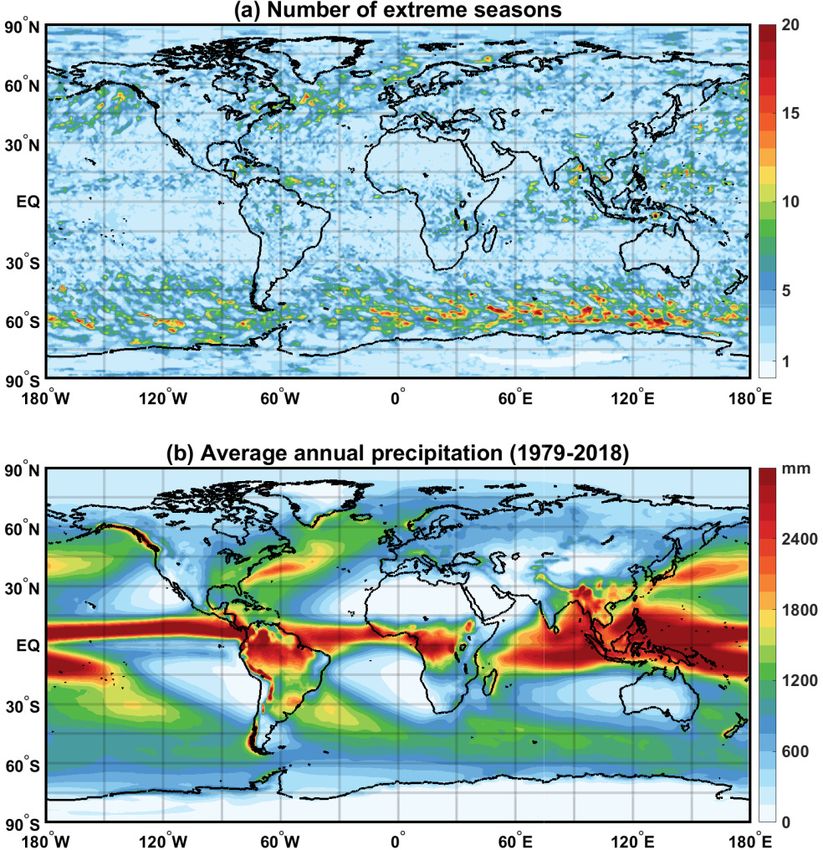
74        E. Flaounas et al.: Extreme wet seasons – their definition and relationship with synoptic-scale weather systems

                                                                         when reaching a region with dynamical or orographic forcing
                                                                         for ascent. Finally, RWB can also lead to long-range trans-
                                                                         port of water vapor, impose large-scale lifting, and reduce
                                                                         static stability in the lower and middle troposphere, thus fa-
                                                                         voring intense precipitation (Martius et al., 2006; de Vries
                                                                         et al., 2018; De Vries, 2020). Sometimes these weather sys-
                                                                         tems occur simultaneously. For instance, RWB may lead to
                                                                         the formation of cyclones that in turn may include WCBs.
                                                                         Therefore, it is an ill-posed problem to determine the sepa-
                                                                         rate contribution of these weather systems to total precipita-
                                                                         tion. However, the objective identification of these weather
                                                                         systems in gridded datasets and counting their seasonal fre-
                                                                         quency of occurrence may provide interesting insights into
                                                                         their role in extreme wet seasons.
                                                                            A common framework has been applied to quantify the
                                                                         co-occurrence of these weather systems and extreme season
                                                                         patches. This co-occurrence is defined for each patch as the
                                                                         number of grid points of the patch that overlap with a specific
                                                                         weather system (note that all our weather systems are de-
                                                                         fined as two-dimensional objects), averaged during the core
Figure 1. Methodological approach in an idealized one-                   period (see Sect. 4.2) of the patch. We then show ratios of
dimensional grid to identify spatial coherences of extreme seasons.      this co-occurrence during the core period of the considered
Red lines show precipitation time series per grid point, vertical        extreme season (e.g., from 10 February to 22 May 1993) with
black lines delineate the identified extreme season per grid point       respect to the climatological co-occurrence (40-year average
and vertical dotted lines depict their central date (only for two sea-   for periods from 10 February to 22 May). A more detailed
sons, to be used as an example in text).                                 method to quantify co-occurrence would require a direct at-
                                                                         tribution of precipitation to each weather feature, as done, for
                                                                         example, by Moore et al. (2019) and De Vries (2020). Nev-
methods described in Sprenger et al. (2017) and references               ertheless, this would increase the complexity, since several
therein. In essence, at every 6-hourly time step of ERAI                 weather systems may interact to synergistically produce high
and for every weather system, the algorithms identify spa-               precipitation amounts, as explained above. Our method thus
tially coherent clusters of grid points that belong to the same          simply quantifies the co-occurrence of weather systems and
weather system, very much like the patches of the extreme                extreme wet seasons in the regions identified as wet season
wet seasons. Table 1 provides a summary of the identifica-               patches. Nevertheless, due to the direct relevance of the four
tion criteria and algorithms used.                                       weather systems for precipitation, our approach provides in-
   All four weather systems are well known to be related to              sight into the role of weather systems in forming extreme
heavy precipitation. Precipitation in the vicinity of these sys-         seasons.
tems is the outcome of a rather complex interaction of dy-
namical processes that differ between the four systems. For
instance, cyclones are known to be responsible for a large               3   Statistical characterization of extreme wet seasons
part of global precipitation (Hawcroft et al., 2012; Pfahl and
Wernli, 2012). The precipitation within cyclones may be at-              Figure 2a shows the number of extreme seasons identified
tributed to a variety of processes such as deep convection in            at each grid point, while Fig. 2b shows, as a reference, the
their center (e.g., in the eyewall of tropical cyclones) and to a        global distribution of annual mean precipitation during the
combination of convective and stratiform precipitation along             40-year period in ERAI. Most regions, in particular most
the frontal structures of extratropical cyclones (Catto and              land and climatologically drier regions, show no more than
Pfahl, 2013). Especially concerning frontal structures, WCBs             one to five extreme wet seasons. However, the number of
can be identified as distinct ascending airstreams extending             identified extreme seasons increases to 5–20 in areas where
through a cyclone warm sector that produce high amounts                  the annual precipitation amount is high, in particular in the
of stratiform and in some cases also convective precipitation            inter-tropical convergence zone (ITCZ) and the midlatitude
(Browning et al., 1973; Flaounas et al., 2017; Oertel et al.,            storm tracks over the eastern North Pacific, the North At-
2019). Precipitation due to WCBs affects both the central re-            lantic and in the Southern Ocean along 60◦ S. This suggests
gion of a cyclone and the associated fronts (Catto et al., 2013;         that in these regions, seasonal precipitation typically varies
Catto and Pfahl, 2013; Pfahl et al., 2014). TMEs foster pre-             only by fractions rather than multiples of the climatologi-
cipitation indirectly by supplying moisture that may rain out            cal mean. Therefore, numerous 90 d periods fall within our

Weather Clim. Dynam., 2, 71–88, 2021                                                          https://doi.org/10.5194/wcd-2-71-2021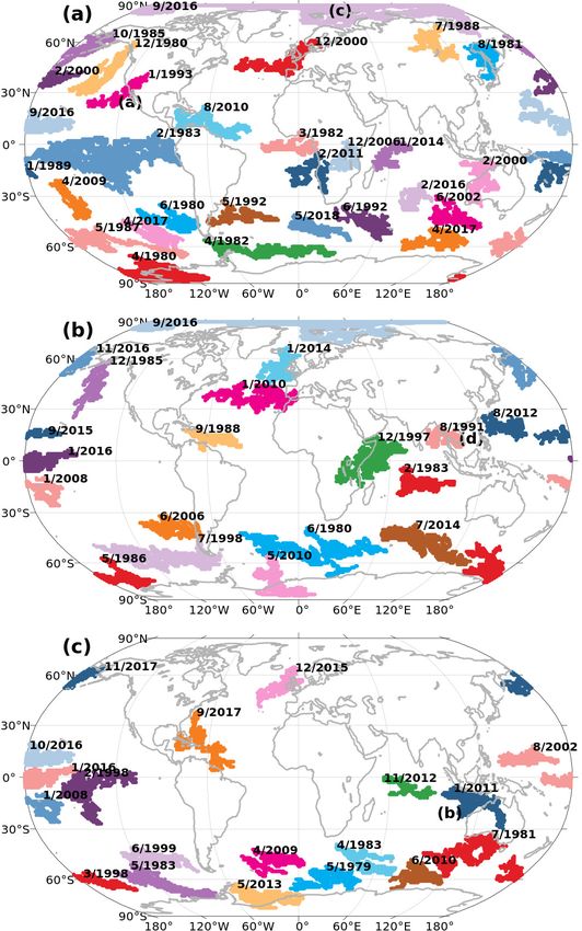
E. Flaounas et al.: Extreme wet seasons – their definition and relationship with synoptic-scale weather systems                           75

Table 1. Short description of the six objectively identified weather systems.

     Cyclones                              Grid points within the outermost sea level pressure contour enclosing one local
                                           minimum (Wernli and Schwierz, 2006)
     Warm conveyor belts                   Grid points overlapping with the ascending part (between 800 and 400 hPa) of air
                                           parcels that rise for at least 600 hPa within 48 h (Madonna et al., 2014a).
     Rossby wave breaking                  Grid points where either potential vorticity (PV) cutoffs or streamers are located.

                                           PV cutoffs: grid points with stratospheric air (PV > 2 PVU), detached from the main
                                           stratospheric body on any isentropic level between 305 and 370 K (Wernli and
                                           Sprenger, 2007)

                                           PV streamers: grid points within narrow filaments of stratospheric air on any
                                           isentropic level between 305 and 370 K (Wernli and Sprenger, 2007)
     Tropical moisture exports (TMEs)      Grid points overlapping with 7 d forward trajectories started from the tropics (20◦ S–20◦ N)
                                           that reach 35◦ latitude in either hemisphere with a horizontal moisture flux of more
                                           than 100 g kg−1 m s−1 (Knippertz and Wernli, 2010)

                                                                          Figure 3. Month during which the central day of the primary ex-
                                                                          treme season occurred at each grid point.

                                                                          extreme wet seasons occur predominantly during boreal and
                                                                          austral summer, when convection triggered by strong solar
                                                                          radiation becomes important (see, for example, Rüdisühli et
                                                                          al., 2020, for Europe). Over midlatitude maritime areas, the
                                                                          extreme seasons occur mainly in boreal and austral winter,
                                                                          when storm tracks are fully developed and extratropical cy-
                                                                          clones tend to be most intense and occur most frequently. In
Figure 2. (a) Global distribution of the number of extreme seasons.       regions where tropical cyclones occur frequently (e.g., in the
(b) Average annual precipitation in a 40-year period (1979–2018).         Caribbean and southern Indian Ocean), the wettest seasons
                                                                          occur in the respective autumn season. For the Arctic, ex-
                                                                          treme seasons occur in late summer and early autumn when
definition of secondary “extreme wet seasons”. These pe-                  sea ice coverage is at its minimum; for Antarctica, however,
riods reach almost the same accumulated precipitation as                  the pattern is very heterogeneous. In the tropics, extreme sea-
the locally wettest period and, therefore, we also choose to              sons are most frequent in regions affected by the latitudi-
use the terminology “extreme wet seasons” for these periods               nal displacements of the ITCZ. However, Fig. 3 shows that
throughout this paper.                                                    the land–sea distinction is not equally sharp in all regions.
   Figure 3 shows the seasonality of the primary extreme sea-             For instance, the west coast of the US, the Iberian Penin-
sons. Color assignment is done according to the month that                sula and the north African coast, as well as Chile and east-
includes the central date of each primary extreme season. In              ern Australia, all experience primary extreme wet seasons
both hemispheres there is a clear shift in seasonality from               in winter. This suggests that such regions are influenced by
oceanic to land regions. Over midlatitude continental areas,              systems that made landfall, such as extratropical cyclones

https://doi.org/10.5194/wcd-2-71-2021                                                          Weather Clim. Dynam., 2, 71–88, 2021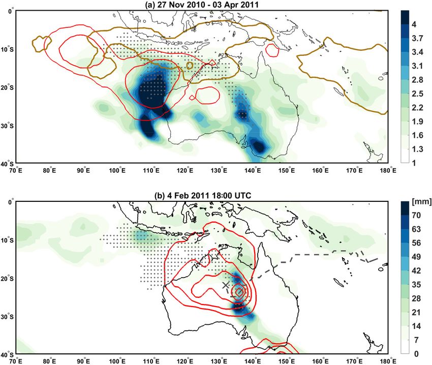
76 E. Flaounas et al.: Extreme wet seasons – their definition and relationship with synoptic-scale weather systems
and atmospheric rivers (Rutllant and Fuenzalida, 1991; Le-
ung and Qian, 2009; Lavender and Abbs, 2012; Flaounas
et al., 2017). Other exceptions from the dominant summer
occurrence of extreme wet seasons over land are several re-
gions in the Northern Hemisphere where extreme seasons
occur in spring, in contrast to summer for their neighbor-
ing continental areas. This is especially observed near Iran,
in the southern part of the Arabian Peninsula, and in east-
ern China and the eastern US. Especially for the east coast
of the US, springtime extreme seasons are conceivably re-
lated to anomalously frequent occurrences of daily extreme
precipitation events (Li et al., 2018).
Next, the extreme seasons are statistically character-
ized. To this end, Fig. 4a shows the ratio of precipitation
amounts during these seasons to climatological, i.e., 40-year-
averaged, values for the same 90 d. Only results for primary
extreme seasons are presented, while results are similar for
secondary seasons. For instance, if a grid point experiences
an extreme season from 10 February to 9 May 1991, then
the value in Fig. 4a corresponds to the ratio of the total pre-
cipitation in this specific period with the precipitation in all
periods in the 40 years from 10 February to 9 May. By def-
inition, extreme seasons have larger precipitation amounts
than the climatology and therefore the amount ratio is every-
where larger than 1. However, Fig. 4a shows that this ratio
strongly varies from close to 1 to more than 6. Comparison
with the climatology in Fig. 2b shows that lower ratios are
found in areas where annual precipitation is high, such as
within the ITCZ (where annual precipitation exceeds, on av-
erage, 2500 mm; see Fig. 2b) and along the midlatitude storm
tracks (roughly between 30 and 60◦ latitude in both hemi-
spheres, where averaged annual precipitation in Fig. 2b is of
the order of 1500 mm). These low precipitation amount ra-
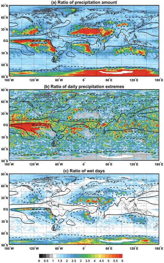
Figure 4. (a) Ratio of precipitation amount of extreme seasons with
tios are consistent with the high numbers of extreme seasons respect to the seasonal average, and (b) the ratio of the number of
in these regions (Fig. 2a). In contrast, high ratios of precipi- daily precipitation extremes included in an extreme season with re-
tation amounts are observed in areas where annual amounts spect to the seasonal average. (c) As (b) but for the number of wet
are low, such as near the poles and in the arid subtropical days. Dashed and solid contours depict annual average precipitation
areas along 30◦ latitude in both hemispheres. The latter ar- of 500 and 1500 mm.
eas are climatologically affected by the descending branch
of the Hadley cell, typically inhibiting precipitation occur-
rence, and therefore an anomalously high seasonal precipita- tremes are defined individually at each grid point as daily
tion amount has the potential to exceed climatological values precipitation values exceeding the 98th percentile of all wet
by a large factor. Finally, Fig. 4a shows that areas character- days in the 40-year dataset, while wet days are defined by
ized by extreme seasons with amount ratios between 2 and 4 daily accumulations that exceed 1 mm. Comparing Fig. 4b
are located between strongly contrasting regions in terms of and c, it appears that the ratios of daily precipitation ex-
annual precipitation amounts (Fig. 2b). It is in these regions tremes and wet days show a contrasting pattern: a high ratio
where spatial anomalies in the occurrence of precipitating of daily precipitation extremes tends to co-occur with a low
weather systems (e.g., due to anomalous cyclone tracks) may ratio of wet days, and vice versa. This is especially evident
play a crucial role in forming extreme seasons. This will be in areas that feature particularly large and small precipita-
discussed in more detail in Sect. 6. tion amounts. For instance, in the ITCZ where precipitation
To gain more statistical insight into the factors that lead is climatologically very frequent, an extreme season may oc-
to extreme seasons, Fig. 4b and c show the ratios of extreme cur due to increased rainfall amounts. This is reflected in the
daily precipitation events and wet days in extreme seasons anomalously high ratios of daily precipitation extremes in ex-
with respect to climatology (evaluated for the same 90 d pe- treme seasons (Fig. 4b). In contrast, in arid areas where rain-
riods as the extreme seasons but in all 40 years). Daily ex- fall occurs rarely (outlined by dashed contours in all panels of
Weather Clim. Dynam., 2, 71–88, 2021 https://doi.org/10.5194/wcd-2-71-2021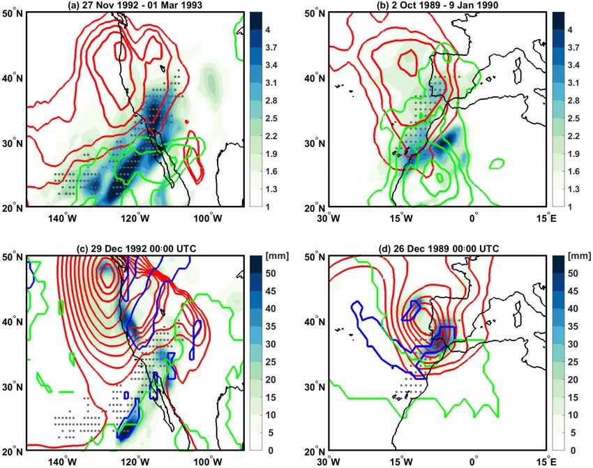
E. Flaounas et al.: Extreme wet seasons – their definition and relationship with synoptic-scale weather systems 77
Fig. 4), a small increase in the number of wet days can be re-
sponsible for a dramatic increase in seasonally accumulated
precipitation. It is thus plausible that the lower the climato-
logical precipitation amounts in an area, the more an extreme
season is characterized by an anomalously high frequency of
wet days. On the other hand, in climatologically wet regions
(such as in the tropics, within the solid contours of Fig. 4), ex-
treme seasons are related to an anomalously high frequency
of daily extremes. Apart from this contrast between climato-
logically wet and dry areas on the globe, some regions have
relatively high ratios of both daily extremes and wet days.
Indeed, when comparing Fig. 4b and c, areas with a high ra-
tio of daily extremes are spatially less constrained than areas
with a high wet-day ratio. This is especially true in the tropics
and midlatitudes (up to 60◦ of latitude), suggesting that daily
precipitation extremes may play a more widespread role in
the occurrence of extreme wet seasons than the number of
wet days.
In both Fig. 4b and c, a large majority of ratios exceeds
the value of 1, suggesting that an extreme season typically
occurs if there is a combination of both more wet days and
more extreme events compared to the seasonal climatology.
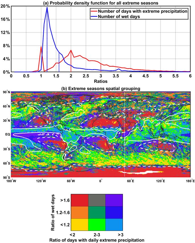
Indeed, Fig. 5a shows the probability density functions of the
ratios of daily precipitation extremes and of wet days for all
extreme seasons at all grid points. Clearly the spread of ratios
of daily extremes is larger than the spread of ratios of wet
Figure 5. (a) Probability density function of the number of ratios
days, with values between 1 and 5 and a median of 2.3 for of daily precipitation extremes and wet days for all extreme seasons
daily extremes and a much narrower distribution with a me- and for all grid points (ratios with respect to the seasonal average).
dian of 1.3 for wet days. Interestingly, the distribution for the Vertical dotted lines correspond to ratios of 1.2, 1.6, 2 and 3. (b) At-
daily extremes is bimodal with peaks near values of 1 and 2, tribution of grid points to nine categories of pairs of ratios of the
respectively, where the first peak is related to arid areas. To number of wet days and of daily precipitation extremes. Dashed and
combine information provided by the two ratios (mean val- solid white contours depict annual average precipitation of 500 and
ues shown in Fig. 4b and c) and their variability (shown in 1500 mm, respectively. Dotted lines in (a) show the category bound-
Fig. 5a), we subjectively defined three ranges for the two aries used in (b).
distributions in Fig. 5a. These ranges are delimited by the
peaks and the 75th percentile of the distributions (depicted
by dashed lines in Fig. 5a). This forms a total of nine bins that where wet-day ratios are close to 1, i.e., where extreme sea-
serve to characterize each grid point according to the ratios of sons occur with roughly the climatological value of wet days.
daily extremes and wet days required to form an extreme sea- Despite the high spatial variability in Fig. 5b, several re-
son (Fig. 5b). For instance, equatorial Africa and the Sahara gional patterns can be distinguished. Areas related to high
are two contrasting regions of frequent and scarce precipita- precipitation amounts (Fig. 2b) and a large number of ex-
tion, respectively. Cyan and light green colors in equatorial treme seasons (Fig. 2a), such as the storm tracks, are de-
Africa indicate a low wet-day ratio of less than 1.2 and a picted by yellow colors in Fig. 5b (e.g., along 60◦ S). These
daily extreme ratio of more than 2. Therefore, in this region, areas are characterized by wet-day ratios of less than 1.2 and
an extreme season requires only slightly more wet days than daily extreme ratios of less than 2. As discussed before, the
in the climatology but at least 2 times more daily extremes. identification of a high number of extreme seasons makes
Before further discussing these patterns, it is noteworthy that it difficult for these seasons to strongly exceed climatology.
13 % of all grid points feature ratios of daily precipitation Other regions that experience high precipitation amounts due
extremes below 1 (Fig. 5a). These values are concentrated in to the ITCZ have a daily extreme ratio exceeding 3 and a
areas of scarce precipitation and are depicted by grey colors low wet-day ratio of less than 1.2 (cyan color), in agreement
in Fig. 4b. For wet days, ratios below 1 are even less com- with the previous discussion of extreme seasons in this re-
mon: they occur only for 3 % of all grid points and typically gion. Extreme seasons with high wet-day and daily extreme
exhibit values between 0.9 and 1 (Fig. 5a). In contrast to daily ratios (purple colors) mostly occur in the transition between
precipitation extremes, these grid points are scattered across areas of high and low climatological amounts of precipitation
areas of frequent precipitation (e.g., ITCZ and storm tracks), (Fig. 2b), for instance in subtropical maritime areas in both
https://doi.org/10.5194/wcd-2-71-2021 Weather Clim. Dynam., 2, 71–88, 2021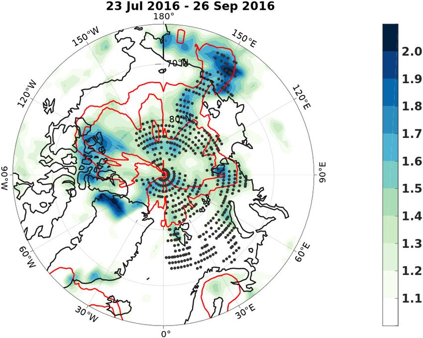
78        E. Flaounas et al.: Extreme wet seasons – their definition and relationship with synoptic-scale weather systems

hemispheres (e.g., the eastern Atlantic and Pacific oceans),
but also in the eastern tropical Pacific. Especially the lat-
ter experiences major El Niño–Southern Oscillation (ENSO)
events, which lead to a strong increase in wet days and daily
extremes. Continental regions in the midlatitudes are mostly
characterized by dark green and orange colors, suggesting
that extreme seasons are characterized by 1.2 to 1.6 more wet
days and less than 3 times as many daily extremes than in the
climatology. It is, however, noteworthy that several coastal
areas have extreme seasons characterized by the highest ra-
tios of wet days and daily extremes (purple colors), for in-
stance Portugal, eastern Australia and Greenland.

4     Portrayal of extreme wet season patches

4.1    The 100 largest patches

The methodology to build patches of grid points with coher-
ent extreme seasons (see Sect. 2.2) has been applied to all
primary and secondary extreme seasons. Figure 6 shows the
100 largest patches in three panels to avoid overlapping. In
these panels, patches are labeled by the month and year of the
average date of all 90 d periods that compose the patches. The
size of the patches in Fig. 6 varies between 1.75 × 10⁶ and
1.86 × 10⁷ km2 . The largest one occurred from January to
March 1983 in the eastern tropical Pacific (Fig. 6a).
   Several patches correspond to or include well-documented
periods of anomalously high precipitation, and some of them
also reflect singular weather events that produced enough
precipitation to characterize a whole 90 d period as an ex-
treme season. For instance, the patches in the western North
Atlantic in Fig. 6a and c correspond to the anomalously ac-
                                                                  Figure 6. The 100 largest patches, labeled with the central month
tive hurricane seasons of 2010 and 2017. In contrast to these     and year of all included extreme seasons. For clarity reasons, all
active hurricane seasons, the patch in the same region in         areas are distributed in three panels and are depicted by different
September 1988 (Fig. 6b) does not correspond to one of            random colors. Four patches are also labeled by a black letter in
the most active hurricane seasons, but rather corresponds to      parenthesis that corresponds to panels in Fig. 7.
the extremely intense Hurricane Gilbert (1988), one of the
deepest hurricanes ever documented with a central pressure
of 888 hPa. Other patches in the tropics agree with major         ranean (Harnik et al., 2014; Sprenger et al., 2017). Other
El Niño and La Niña phases, such as the ones in 1982–1983,        patches that depict known cases affected northwestern Aus-
1997–1998 and 2015–2016 in the central Pacific (Fig. 6a–c),       tralia in 2000 and 2011 (Fig. 6a and c), associated with en-
and with ENSO-related extreme wet seasons in austral sum-         hanced cyclone activity and a strong Mascarene high (Feng
mer 2010–2011 (Fig. 6c; Ratna et al., 2014).                      et al., 2013). Another example is discernible in the eastern
   Within the storm tracks of the Northern Hemisphere,            Antarctic where anomalously high precipitation occurred in
Fig. 6b shows two patches that are associated with anoma-         autumn 1980 (Fig. 6a) as discussed by van Ommen and Mor-
lous variability of the polar jet: the first one corresponds to   gan (2010). All these examples provide insight into the vari-
the extremely wet winter in the UK in 2013–2014, when an          ability of the specific weather systems and/or climatological
anomalously strong and persistent jet stream led to a series of   features that can lead to extreme wet seasons. This relation-
extratropical cyclones hitting the region (Davies, 2015; Mc-      ship will be analyzed more systematically in the following
Carthy et al., 2016; Priestley et al., 2017). The second patch    sections.
in the central North Atlantic along 35◦ N in winter 2009–
2010 is associated with an anomalous southward deviation
of the North Atlantic jet that led to a high frequency of
TMEs and enhanced precipitation over the western Mediter-

Weather Clim. Dynam., 2, 71–88, 2021                                                    https://doi.org/10.5194/wcd-2-71-2021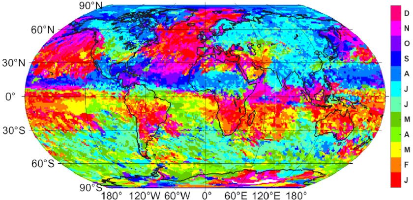
E. Flaounas et al.: Extreme wet seasons – their definition and relationship with synoptic-scale weather systems                                79

Figure 7. Panels (a–d) depict exemplary patches, with each label corresponding to the respective panel’s letter in Fig. 6. Time periods on the
abscissa span from the earliest (day 1) to the latest date (e.g., day 170 in a) of all extreme seasons of the grid points that compose each patch.
The upper part of each panel shows time series of daily precipitation, accumulated for all grid points that compose the patch. Given that the
patch period on the abscissa is composed by non-identical extreme seasons per grid point, the time series in the middle of each panel shows
the fraction of the extreme season patch that includes the respective day. The lower part of the panel marks each day by a vertical line if a
weather system overlapped with the patch (see text): red for cyclones, blue for WCBs, green for TMEs and brown for RWB. Central date
and average latitude and longitude of each of the four patches are shown under the panels.

4.2   Four example patches and definition of their core                    Fig. 6c). Figure 7c is for a patch in the Arctic in late sum-
      period                                                               mer 2016 (label c in Fig. 6a), and Fig. 7d presents an exam-
                                                                           ple in the Asian summer monsoon region in 1991 (label d
The patches provide a spatial dimension to the identified ex-              in Fig. 6b). The time period in each panel of Fig. 7 spans
treme seasons. However, with our approach (see Sect. 2.2)                  the earliest day (referred to as day 1) and the latest day (e.g.,
and especially for patches with many grid points, the com-                 day 200 in panel a) from all 90 d extreme season periods that
bined period of extreme seasons (identified at every grid                  contribute to the considered patch. For each patch, three time
point) can extend over a significantly longer period than 90 d.            series are shown in the panels of Fig. 7: (i) the upper graphs
Such patches tend to be located in regions where many sec-                 show time series of daily precipitation summed over all grid
ondary extreme seasons were identified, such as in the South-              points that include the same day within their corresponding
ern Ocean. This is plausibly due to numerous secondary ex-                 90 d extreme seasons. For instance, let a certain day in the
treme season periods at neighboring grid points that can ful-              abscissa be included in the 90 d extreme seasons of 15 out of
fill the temporal overlap criterion of 68 d (Sect. 2.2). In order          30 grid points that compose a patch. Then the upper graph of
to make the attribution to weather systems comparable across               Fig. 7 shows the sum of daily precipitation in these 15 grid
patches, the aim is here to define for each patch a “core pe-              points for that certain date. (ii) The middle graphs show what
riod” that contains most of the area-integrated precipitation.             we call the “percentage of contributing grid points”, i.e., the
    To illustrate this approach, we show detailed information              percentage of grid points of the patch that contain the con-
about four selected example patches (labeled as a–d in Fig. 6)             sidered day in their 90 d extreme season period. (iii) The bot-
in Fig. 7. The central date, latitude and longitude of these               tom graphs indicate the occurrence of weather systems, as
patches are shown at the bottom of each panel. Figure 7a pro-              discussed below. For instance, the patch in the western US
vides information on an elongated, tongue-like-shaped patch                has a peak of area-integrated precipitation of ∼ 23 × 1012 L
that affected the US west coast in winter 1992–1993 (label a               on day 52. This value corresponds to the sum of daily pre-
in Fig. 6a). Figure 7b corresponds to a rather large patch that            cipitation from all grid points of the patch (the percentage of
covers parts of Australia in summer 2010–2011 (label b in

https://doi.org/10.5194/wcd-2-71-2021                                                             Weather Clim. Dynam., 2, 71–88, 2021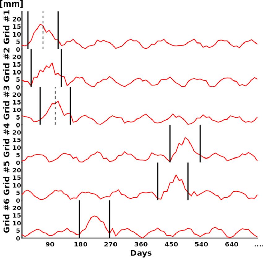
80       E. Flaounas et al.: Extreme wet seasons – their definition and relationship with synoptic-scale weather systems

contributing grid points is 100 %); i.e., this day is included in    Fig. 7a–c to better understand the contribution of the four
all 90 d extreme season periods of the grid points that com-         weather systems to the precipitation in these extreme season
pose this patch.                                                     patches.
   This visualization is now helpful to explain how a “core
period” can be determined for each patch. All four examples
show that at the beginning and near the end of a patch pe-           5     Examples of how weather systems contribute to
riod, only a few grid points contribute to the patch and the               extreme wet seasons
area-integrated precipitation values are lower in these peri-
                                                                     5.1    Cold season patches in the subtropical–midlatitude
ods. Also, in all cases, there is a more or less central time
                                                                            transition zone
interval when (almost) all grid points contribute to the patch,
and in these intervals the integrated precipitation is largest.      The time series for the subtropical-to-midlatitude patch in
We therefore define the core period as the longest period            Fig. 7a exhibits distinct peaks in the 96 d core period. Several
during which at least 25 % of the respective grid points con-        of these peaks coincide with cyclones and TMEs, as shown
tribute to the patch. Considering again the western US patch         in the bottom graph by the red and green lines, respectively.
(Fig. 7a), the so-defined core period extends from day 8 to          Figure 8 provides insight into the complex relationship be-
day 104; for the monsoon patch (Fig. 7d) it becomes much             tween precipitation, cyclones and TMEs for this patch, but
longer from day 6 to day 141. It is noteworthy that core pe-         also for another patch of similar latitudinal extent and ori-
riods may not include days with locally intense precipitation        entation that affected the Iberian Peninsula in late autumn
events that do not affect a large fraction of the patch area. The    1989 (note that this additional patch is not depicted in Fig. 7).
intention of the core period is to consider precipitation in the     Figure 8a and b show that the patches present core period
entire larger-scale area of the extreme season patch, and to         precipitation amounts that exceed climatological values by
identify the time period that is most important for precipi-         a factor that varies from 2 to 5. In fact, the northern parts
tation in the patch as a whole. Core periods of patches may          of the patches are related to positive anomalies of cyclone
last longer than 90 d, i.e., the default time period that was ini-   occurrence of 5 % to 15 %. On the other hand, the south-
tially used to define extreme seasons at individual grid points.     ern parts of both patches are co-located with climatological
In fact, further analysis shows that for all 3734 patches, the       anomalies of northern extensions of TME occurrences of the
median and the 75th and 95th percentile values of the core           same order as for cyclones. It thus seems that cyclones act
period durations amount to 99, 114 and 147 d, respectively.          in synergy with TMEs to produce the large amounts of pre-
Assigning a flexible core period duration to each patch allows       cipitation within the patch. Blue lines in the lower graph of
extreme wet season patches to take into account the climato-         Fig. 7a coincide with prominent peaks of area-integrated pre-
logical characteristics of the different regions on the globe.       cipitation in the US patch, for instance on day 40. Hence,
For instance, core periods in the tropics (Fig. 7d) may last         despite their rather infrequent occurrence, WCBs may still
for more than 100 d, corresponding to the duration of an in-         constitute a key dynamical ingredient to extreme seasonal
tense monsoon season.                                                precipitation amounts. To underline this point, Fig. 8c and d
   Finally, we now investigate the occurrence of the four ob-        show daily precipitation, sea level pressure, and the spatial
jectively identified weather systems (Table 1) during the core       extent of TMEs and of ascending WCBs for peak precip-
periods of the four example patches. The bottom graphs in            itation days during the US patch (day 40, i.e., 29 Decem-
the panels of Fig. 7 show colored lines for each weather sys-        ber 1992) and the Iberian patch (26 December 1989), re-
tem type indicating the days when a system overlaps with             spectively. In both cases, the local maxima of daily precip-
parts of the patch. Three shadings of colors are used to in-         itation exceeding 50 mm coincide with WCBs in the warm
dicate whether 5 % to 33 % of the grid points of the patch           sectors of deep cyclones. Such amounts represent large con-
overlap with the weather system (light shading), or whether          tributions to the total precipitation during the patches’ core
this percentage amounts to 33 %–66 % (medium shading), or            period, and thus the two examples suggest links between pro-
to more than 66 % (dark shading). For instance, dark green           cesses on the weather timescale (extratropical cyclones and
bars in Fig. 7a denote days when TMEs overlap with more              their associated WCBs) and seasonal-scale extreme precip-
than 66 % of the western US patch. WCBs never exceed 33 %            itation. In fact, both these extreme wet season patches are
in Fig. 7 and thus only light blue shading is visible. This pro-     in areas where cyclones and WCBs contribute frequently to
vides qualitative information about the occurrence and rele-         intense precipitation (Pfahl et al., 2014; their Fig. 8).
vance of a weather system to the precipitation in the patch.
Indeed, all four identified weather systems are known to be          5.2    Warm season patch in the tropical–subtropical
climatologically highly relevant for heavy rainfall. It is, how-            transition zone
ever, noteworthy that large patches may exhibit several local
maxima of precipitation on a given day, but not all of them          Figure 9a provides more information about the northern Aus-
necessarily overlap with one of the weather systems. In the          tralian patch in summer 2010–2011, previously introduced
following, we further investigate the exemplary patches of           in Fig. 7b. This patch covers large parts of the maritime ar-

Weather Clim. Dynam., 2, 71–88, 2021                                                      https://doi.org/10.5194/wcd-2-71-2021
E. Flaounas et al.: Extreme wet seasons – their definition and relationship with synoptic-scale weather systems 81 Figure 8. (a) Ratio of accumulated precipitation during the period 27 November 1992 to 1 March 1993 with respect to climatological values for the same time period (in color) for an extreme wet season patch affecting the US west coast (dotted area). Red (green) contours show areas with positive anomalies of cyclone (TME) occurrences with respect to climatology. Contours start from 5 % and have a 5 % interval. (b) As (a) but for the period 2 October 1989 to 9 January 1990 for an extreme wet season patch affecting the Iberian Peninsula (dotted area). (c) 24 h accumulation of precipitation from 12:00 UTC on 28 December to 12:00 UTC on 29 December 1992 (in color). Red contours show sea level pressure at 00:00 UTC on 29 December 1992 (starting from 1015 hPa and with a step of −3 hPa). Green contours show areas with TMEs and blue contours show areas with WCB ascent. (d) As in (c) but at 00:00 UTC on 26 December 1989. eas northwest of Australia and includes a tongue-like exten- and enhanced precipitation by RWB, but also due to the fre- sion to the center of the continent. Large parts of the patch quent occurrence of cyclones in the northwest of Australia overlap with areas with high cyclone frequencies, especially plus the single, prominent system of Tropical Cyclone Yasi. close to the west coast at 115◦ E, 20◦ S. In this part of the Therefore, the spatial extension of extreme season patches patch, a positive cyclone frequency anomaly of 10 % to 20 % can be due to a combination of specific weather systems that is collocated with seasonal precipitation amounts of more occur in different subregions of the patch. than 5 times the climatological value. On the other hand, the northern part of the patch is located within the ITCZ of 5.3 The summer 2016 patch in the Arctic the Australian summer, a region where Coriolis forces are too weak to favor cyclogenesis. However, Fig. 9a shows that Figure 7c depicts a large patch that covers the eastern Arctic RWB events along the northern part of the patch took place in late summer 2016 (dotted area in Fig. 10). Figure 10 shows during its core period with an anomalous occurrence of 20 % that a large part of this patch is related to an anomalous occur- with respect to climatology. These RWB events can signifi- rence of cyclones of 5 % to 10 % with respect to climatology. cantly contribute to the formation of precipitation by reduc- The region with anomalously frequent cyclones (red contour) ing the static stability beneath and forcing vertical ascent. agrees with the southward extension of the patch into Siberia Further analysis showed that the narrow continental near 150◦ E and with an anomalously high precipitation ex- tongue of the patch is associated with a specific event: the cess compared to climatology, with a ratio of more than 1.7. landfall of Tropical Cyclone Yasi (track is shown in Fig. 9b). Figure 7c shows that several prominent peaks in the precipi- Yasi made landfall at the Australian east coast and moved tation time series coincide with WCBs and RWB events, sim- into the continent in February 2011, contributing strongly ilarly to the subtropical patch in Fig. 7a. The year 2016 has to the precipitation peak around day 165 in Fig. 7b. Con- been recorded as the warmest in the last decades in the Arc- sequently, this Australian patch has been formed through the tic and was characterized by anomalously low sea-ice extent combined contribution of climatological features (the ITCZ) and overall positive sea surface temperature anomalies that https://doi.org/10.5194/wcd-2-71-2021 Weather Clim. Dynam., 2, 71–88, 2021
82       E. Flaounas et al.: Extreme wet seasons – their definition and relationship with synoptic-scale weather systems

Figure 9. (a) Ratio of accumulated precipitation during the period 27 November 2010 to 3 April 2011 with respect to climatological values
for the same time period (in color) for an extreme wet season patch affecting Australia (dotted area). Red (brown) contours show areas with
positive anomalies of cyclone (RWB) occurrences with respect to climatology (shown are anomalies of 10 % and 20 % for cyclones and 20 %
for RWB). (b) 24 h accumulation of precipitation from 18:00 UTC on 3 February to 18:00 UTC on 4 February 2011 (in color). Red contours
show sea level pressure at 18:00 UTC on 4 February 2011 (starting from 1006 hPa and with steps of −2 hPa). The grey dashed line shows
the track of Tropical Cyclone Yasi, while its position of cyclolysis is represented by the cross symbol.

enhanced evaporation and consequently precipitation (Simp-              matology. In addition, the right-hand panels of Fig. 11 show
kins, 2017; Overland et al., 2019; Petty, 2018). Evidently,             the latitudinal distribution of the overlapping frequency ra-
such conditions can lead to extreme wet seasons in the east-            tios. They were calculated by zonally averaging the ratios of
ern Arctic and are similar to the ones leading to a rainier fu-         all patches within ±7.5◦ of each latitude degree. Figure 11
ture regime in the Arctic region (Bintanja and Andry, 2017).            provides a global view of the relationship between patches
                                                                        and the occurrence of the identified weather systems. To pro-
                                                                        vide a seasonal perspective of Fig. 11, but also to increase
6    The contribution of weather systems to extreme wet                 the figure clarity, we include in the Supplement four versions
     seasons: a global view                                             of Fig. 11, each showing only patches with a central date
                                                                        of their core period in boreal winter (DJF), spring (MAM),
Following the three examples of the previous section, we
                                                                        summer (JJA) and autumn (SON).
quantified the occurrence of the four objectively identified
                                                                           Figure 11a reveals the importance of cyclones for the for-
weather systems during all the 3734 identified patches. To
                                                                        mation of precipitation in extreme wet seasons. Most lati-
this end, we counted the number of days with an overlap of
                                                                        tudes, except those in the tropics, are covered by patches
each weather system with the patch during its core period.
                                                                        with frequency ratios of at least 1.2. The latitudinal distribu-
In order to then estimate whether these numbers are anoma-
                                                                        tion of these ratios shows two local maxima in the subtrop-
lous compared to climatology, this process was repeated for
                                                                        ics close to 30◦ latitude. The origin of these maxima cannot
the same dates and grid points as for the core period, but for
                                                                        be attributed clearly to tropical, subtropical or extratropical
all 40 years of our dataset. The ratio then defines the over-
                                                                        cyclones. Nevertheless, Fig. 3 shows that these regions ex-
lapping frequency ratio of a patch with respect to climatol-
                                                                        perience their extreme seasons in the colder months of the
ogy, and results are presented in Fig. 11. For instance, orange
                                                                        year, and thus it is rather unlikely that tropical cyclones may
patches in Fig. 11a are overlapping about 2.5 times more of-
                                                                        contribute to their formation. Indeed, Fig. 11a shows that
ten with cyclones during their core periods than in the cli-

Weather Clim. Dynam., 2, 71–88, 2021                                                          https://doi.org/10.5194/wcd-2-71-2021
E. Flaounas et al.: Extreme wet seasons – their definition and relationship with synoptic-scale weather systems 83
higher than the one of cyclones (Fig. 11a). This suggests that
extreme seasons within the storm tracks are not formed due
to a higher frequency of cyclones but due to a higher fre-
quency of WCBs. Indeed, WCBs essentially contribute to the
enhancement of seasonal precipitation and thus to the forma-
tion of extreme seasons in midlatitude oceanic regions, but
also in continental and polar regions. However, it is notewor-
thy that the climatological infrequency of WCBs, especially
in the polar regions (e.g., Fig. 7c; see also Madonna et al.,
2014a), can result in the high ratios in Fig. 11b, even if few
WCBs occurred during the extreme season.
TMEs correspond to the transport of moist air from the
tropics into the extratropics. Therefore, TMEs are expected
to favor higher amounts of precipitation whenever they reach
areas of strong ascending motion in higher latitudes. Indeed,
Fig. 11c shows several patches with high TME frequency ra-
tios, especially along 60◦ S, but also in the continental ar-
Figure 10. Ratio of accumulated precipitation during the period eas of Asia and North America. A quasi-constant zonal av-
23 July to 26 September 2016 with respect to climatological val-
erage of 1.1 is observed in the midlatitudes (right panel of
ues for the same time period (in color). Red contours show areas
Fig. 11c), suggesting that TMEs may contribute to the for-
with positive anomalies of cyclone occurrences with respect to cli-
matology (shown are contours of 5 % and 10 %). The spatial extent mation of extreme seasons in the extratropics. However, this
of the patch is represented by the dotted area. contribution is expected to be weaker than the one from cy-
clones and WCBs. Occasionally, TMEs contribute to the for-
mation of extreme seasons in the Arctic, but the high ratios
in this region (Fig. 11c) result from only a few events during
several patches in the subtropics have cyclone frequency ra- the extreme seasons and even fewer in the climatology.
tios of more than 2, and in some cases even more than 4. Finally, Fig. 11d shows generally low values of overlap-
Patches with high ratios occur in particular in subtropical ping ratios of RWB, rarely exceeding values of 1.5. This
oceanic regions, in transitional areas between climatologi- is a consequence of the fact that RWB is climatologically
cally high and low precipitation amounts (Fig. 2a). These re- frequent, and thus the RWB frequency ratios cannot be as
gions are also characterized by an anomalously high num- large as the ones of cyclones and WCBs, two weather sys-
ber of wet days and daily extremes (Fig. 5b). This result tems with a lower climatological frequency. The latitudinal
suggests that cyclones occurring equatorward of the clima- profile of RWB frequency ratios (right panel of Fig. 11d)
tological storm tracks are a key ingredient for extreme wet presents two local minima, both in the midlatitudes of the
seasons since they trigger anomalously frequent precipita- two hemispheres where RWB is particularly frequent. How-
tion extremes in these regions (see also Pfahl and Wernli, ever, when elongated RWB-related PV streamers occasion-
2012). Low ratios in Fig. 1a occur along the Equator due ally intrude into the tropics, then extreme precipitation may
to the absence of cyclones, but also within the storm track be triggered (Knippertz, 2007). Because such events are rare
regions (e.g., along 60◦ S). Especially in the Southern Hemi- and intense, a maximum of RWB ratios occurs in the trop-
sphere, the right panel of Fig. 11a shows that ratios decrease ics. It is plausible that extensions of PV streamers into the
monotonically from 1.45 at 30◦ S, to 1.1 at 60◦ S. This result tropics lead to daily extreme events, a necessary ingredient
suggests that the closer a patch is located to a climatological for the formation of extreme seasons in these latitudes (e.g.,
storm track, the more unlikely it is for this patch to overlap Figs. 4b and 5b). Nevertheless, other weather systems or con-
with more cyclones than in the climatology. The same also ditions than RWBs, cyclones and WCBs might be also in-
holds in the Northern Hemisphere in the western North At- volved in forming daily precipitation extremes in the tropics
lantic and in the eastern North Pacific between 30 and 60◦ N. and thus be responsible for the formation of extreme sea-
WCBs are directly related to the occurrence of cyclones sons (e.g., a very strong ITCZ or warmer sea surface tem-
and can contribute significantly to extreme precipitation peratures). Finally, in polar latitudes there are relatively high
events (e.g., Pfahl et al., 2014; Oertel et al., 2019). There- frequency ratios of RWB that may be directly related to the
fore, Fig. 11a and b are expected to be similar. This is partly high frequency ratios of WCBs in the same areas (Fig. 11b),
confirmed by the latitudinal distribution of WCB ratios with especially in the Southern Hemisphere. Indeed, WCBs are
peaks in the subtropics at 30◦ S and 25◦ N, similarly to the known to deepen the ridges in a poleward direction and thus
zonal averages of cyclone ratios. However, Fig. 11a and b to significantly contribute to RWB (e.g., Grams et al., 2011;
also present considerable differences. For instance, the fre- Madonna et al., 2014b).
quency ratio of WCBs along 60◦ S (Fig. 11b) is significantly
https://doi.org/10.5194/wcd-2-71-2021 Weather Clim. Dynam., 2, 71–88, 2021You can also read