Ocean phosphorus inventory: large uncertainties in future projections on millennial timescales and their consequences for ocean deoxygenation ...
←
→
Page content transcription
If your browser does not render page correctly, please read the page content below
Earth Syst. Dynam., 10, 539–553, 2019
https://doi.org/10.5194/esd-10-539-2019
© Author(s) 2019. This work is distributed under
the Creative Commons Attribution 4.0 License.

            Ocean phosphorus inventory: large uncertainties in
            future projections on millennial timescales and their
                  consequences for ocean deoxygenation
            Tronje P. Kemena, Angela Landolfi, Andreas Oschlies, Klaus Wallmann, and Andrew W. Dale
           GEOMAR Helmholtz Centre for Ocean Research Kiel, Düsternbrooker Weg 20, 24105 Kiel, Germany
                                Correspondence: Tronje P. Kemena (tkemena@geomar.de)

                                  Received: 8 August 2018 – Discussion started: 2 October 2018
                          Revised: 13 June 2019 – Accepted: 12 July 2019 – Published: 6 September 2019

       Abstract. Previous studies have suggested that enhanced weathering and benthic phosphorus (P) fluxes, trig-
       gered by climate warming, can increase the oceanic P inventory on millennial timescales, promoting ocean
       productivity and deoxygenation. In this study, we assessed the major uncertainties in projected P inventories
       and their imprint on ocean deoxygenation using an Earth system model of intermediate complexity for the same
       business-as-usual carbon dioxide (CO2 ) emission scenario until the year 2300 and subsequent linear decline to
       zero emissions until the year 3000. Our set of model experiments under the same climate scenarios but differing
       in their biogeochemical P parameterizations suggest a large spread in the simulated oceanic P inventory due
       to uncertainties in (1) assumptions for weathering parameters, (2) the representation of bathymetry on slopes
       and shelves in the model bathymetry, (3) the parametrization of benthic P fluxes and (4) the representation of
       sediment P inventories. Considering the weathering parameters closest to the present day, a limited P reservoir
       and prescribed anthropogenic P fluxes, we find a +30 % increase in the total global ocean P inventory by the
       year 5000 relative to pre-industrial levels, caused by global warming. Weathering, benthic and anthropogenic
       fluxes of P contributed +25 %, +3 % and +2 %, respectively. The total range of oceanic P inventory changes
       across all model simulations varied between +2 % and +60 %. Suboxic volumes were up to 5 times larger than
       in a model simulation with a constant oceanic P inventory. Considerably large amounts of the additional P left the
       ocean surface unused by phytoplankton via physical transport processes as preformed P. In the model, nitrogen
       fixation was not able to adjust the oceanic nitrogen inventory to the increasing P levels or to compensate for the
       nitrogen loss due to increased denitrification. This is because low temperatures and iron limitation inhibited the
       uptake of the extra P and growth by nitrogen fixers in polar and lower-latitude regions. We suggest that uncer-
       tainties in P weathering, nitrogen fixation and benthic P feedbacks need to be reduced to achieve more reliable
       projections of oceanic deoxygenation on millennial timescales.

1   Introduction                                                  global scales (Tyrrell, 1999). Thus, changes in oceanic phos-
                                                                  phorus (P) inventories are also hypothesized to substantially
The oxygen balance in the ocean is regulated by physi-            affect oceanic oxygen inventories on millennial timescales
cal supply and the biological consumption. Warming has            (Tsandev and Slomp, 2009; Palastanga et al., 2011; Monteiro
been found to be a major driver of oceanic oxygen vari-           et al., 2012). Elevated supply of P to the ocean stimulates
ability, acting via changes in ocean solubility and indirect      production and export of organic matter and deoxygenation,
changes in circulation and biological production and respi-       which possibly drives more intense oxygen depletion in the
ration (Battaglia and Joss, 2018; Levin, 2018; Oschlies et        oxygen deficient zones and along the continental margins,
al., 2018; Yamamoto et al., 2015). Phosphorus is consid-          with release of additional P from sediments turning anoxic
ered the ultimate limiting nutrient for ocean productivity at     (Van Cappellen and Ingall, 1994; Palastanga et al., 2011).

Published by Copernicus Publications on behalf of the European Geosciences Union.
540                                                                        T. P. Kemena et al.: Ocean phosphorus inventory

Such a positive feedback was discussed for a global warm-        5-fold increase in the suboxic water volume (dissolved oxy-
ing scenario under present-day conditions (Niemeyer et al.,      gen (O2 ) concentrations less than 5 mmol m−3 ) on millennial
2017) as well as for large-scale deoxygenation events in the     timescales. Here, we build on this study and test the sensi-
Cretaceous era, the so-called oceanic anoxic events (OAEs)       tivity of the marine P and O2 inventories to changes in P
(Tsandev and Slomp, 2009; Monteiro et al., 2012; Ruval-          weathering, benthic and anthropogenic fluxes under the same
caba Baroni et al., 2014). For the Cretaceous, it has been       future scenario on millennial timescales. We aim to provide
suggested that atmospheric carbon dioxide (CO2 ) concentra-      better constraints on future ocean deoxygenation and assess
tions as high as 1000 to 3000 ppmv, driven by enhanced CO2       the biogeochemical feedbacks triggered by P addition. In
outgassing from volcanic activity (Jones and Jenkyns, 2001;      Sect. 2, we present the experimental design and the model
Kidder and Worsley, 2012), have triggered OAEs (Damsté           parameterizations of continental P weathering and of benthic
et al., 2008; Méhay et al., 2009; Bauer et al., 2017). The       P release. In Sect. 3, we assess uncertainties in P fluxes due to
warmer climate during past OAEs increased weathering on          different assumptions about the P weathering fluxes, different
land (Blättler et al., 2011; Pogge von Strandmann et al.,        model formulations of benthic P burial and improved repre-
2013), leading to an enhanced supply of nutrients, in partic-    sentation of bathymetry and anthropogenic P fluxes. Conse-
ular P, increasing the oceanic nutrient inventory and driving    quences for deoxygenation and for the biogeochemical cy-
the positive feedback mentioned above. Furthermore, the en-      cling of nutrients are discussed.
hanced release of P from sediments was suggested to main-
tain high levels of productivity in the Cretaceous ocean (Mort
                                                                 2     Model and experimental design
et al. 2007; Kraal et al. 2010), which would contribute to the
development of OAEs. Evidence in the palaeorecord indi-          2.1    Model
cates that the Earth has experienced several OAEs with large-
scale anoxia, euxinia and mass extinctions (Kidder and Wors-     We applied the University of Victoria (UVic) Earth sys-
ley, 2010).                                                      tem model (ESM) version 2.9 (Weaver et al., 2001), which
   Could such OAEs also appear in the near future under con-     has been used in several studies to investigate ocean oxy-
temporary global warming? High CO2 concentrations in the         gen dynamics (Schmittner et al., 2007; Oschlies et al.,
atmosphere seem to be one driver for initiating OAEs and         2008; Getzlaff et al., 2016; Keller et al., 2016; Landolfi et
ocean deoxygenation. Projected anthropogenic CO2 emis-           al., 2017). The UVic model consists of a terrestrial model
sions may lead to atmospheric CO2 concentrations exceed-         based on TRIFFID and MOSES (Meissner et al., 2003),
ing 1000 ppmv at the beginning of the 22nd century if emis-      an atmospheric energy–moisture balance model (Fanning
sions continue to increase in a business-as-usual scenario       and Weaver, 1996), a sea-ice model (Bitz and Lipscomb,
(Meinshausen et al., 2011). Although anthropogenic CO2           1999) and the general ocean circulation model MOM2
emissions occur over a short period compared to the long-        (Pacanowski, 1996). Horizontal resolution of all model com-
term and relatively constant volcanic CO2 emissions dur-         ponents is 1.8◦ latitude × 3.6◦ longitude. The ocean model
ing OAEs (Kidder and Worsley, 2012), elevated atmospheric        has 19 layers with layer thicknesses ranging from 50 m for
CO2 concentrations will persist for many millennia (Clark        the surface layer to 500 m in the deep ocean. The marine
et al., 2016). This may provide the conditions for long-term     ecosystem was represented by a nutrients–phytoplankton–
climate change and large-scale deoxygenation. There is thus      zooplankton–detritus (NPZD) model (Keller et al., 2012).
some concern that anthropogenic CO2 emissions could po-          Organic matter transformations (production, grazing, degra-
tentially trigger another OAE (Watson et al., 2017). Yet, Kid-   dation) were parameterized using fixed stoichiometric molar
der and Worsley (2012) argue that emissions of global fossil     ratios (C : N : P, 106 : 16 : 1) and directly related to the pro-
fuel reserves are insufficient to drive a modern OAE but may     duction and, in oxygenated waters, utilization of O2 (O : P,
instead lead to widespread suboxia.                              160). When O2 is depleted in the model, organic matter is
   During climate warming, ocean productivity could switch       respired using nitrate (NO−    3 ) (i.e. microbial denitrification).
from P to nitrogen (N) limitation (Saltzman, 2005). N lim-       An O2 concentration of 5 mmol m−3 was used as the switch-
itation could arise from enhanced denitrification in a more      ing point from aerobic respiration to denitrification. Sedi-
anoxic ocean, but at the same time low N-to-P ratios would       mentary denitrification was not considered in this model con-
be expected to stimulate N2 fixation by diazotrophs (Kuypers     figuration so that water column denitrification and N2 fix-
et al., 2004). N2 fixation in regional proximity with oxy-       ation dictate the oceanic N balance. No explicit iron cy-
gen minimum zones (OMZs) can lead to net N losses due            cle was simulated and iron limitation was approximated
to mass balance constraints (Landolfi et al., 2013), which       with prescribed seasonally varying dissolved iron concen-
may even reverse the net effect of N2 fixation on the nitro-     trations (Keller et al., 2012). Parameterizations of benthic
gen inventory. Recently, Niemeyer et al. (2017) showed in a      and weathering fluxes of P were extended from the study of
model study that P weathering and sedimentary P release in       Niemeyer et al. (2017). A calcium carbonate sediment model
a business-as-usual CO2 -emission (RCP8.5) scenario could        (Archer, 1996) and a parameterization for silicate and car-
strongly enlarge the marine P inventory and lead to a 4- to      bonate weathering (Meissner et al., 2012) were applied in all

Earth Syst. Dynam., 10, 539–553, 2019                                                www.earth-syst-dynam.net/10/539/2019/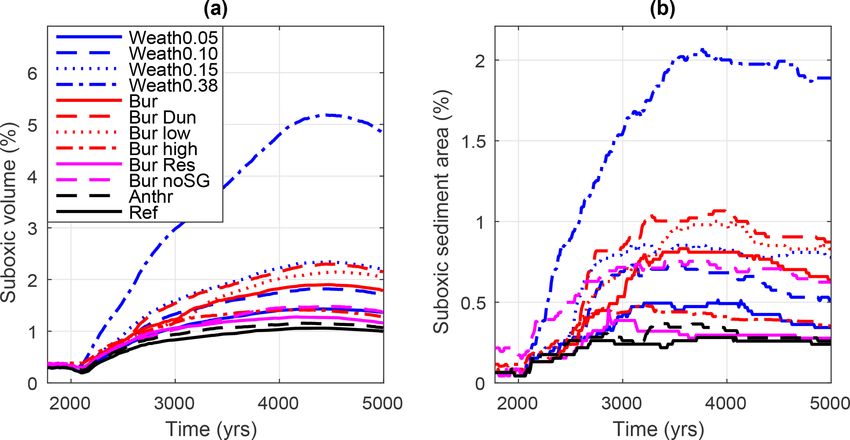
T. P. Kemena et al.: Ocean phosphorus inventory                                                                               541

simulations. When P weathering and anthropogenic P fluxes          lief Data (ETOPO2v2) 1 (National Geophysical Data Cen-
were applied (see Sect. 2.2), the global P flux was distributed    ter, 2006). ETOPO2v2 has a horizontal resolution of 2 min,
over all river basins, in every grid box, weighted by river dis-   which is fine enough to adequately represent continental
charge rates.                                                      shelves and slopes. The coarse standard model bathymetry
                                                                   in the UVic model has a horizontal resolution of 1.8◦ lati-
                                                                   tude × 3.6◦ longitude.
2.2   Experimental design                                             P burial in the sediment (BURP ) was determined in ev-
                                                                   ery grid box with sediment from the difference between the
In total, 12 different model simulations were performed to
                                                                   simulated detritus P rain rate to the sediment (RRP ) and the
explore the range of uncertainties for the long-term devel-
                                                                   benthic release of dissolved inorganic P from the sediment
opment of the oceanic P inventory (Table 1). Each simu-
                                                                   (BENP ):
lation started from an Earth system state close to equilib-
rium under pre-industrial atmospheric CO2 concentrations,          BURP = RRP − BENP ,                                         (1)
prescribed wind fields and present-day orbital forcing. Spin-
up runs lasting 20 000 simulation years or longer were made        where RRP is the detritus flux from the ocean (in P units).
for each simulation to reach equilibrium. In the spin-up runs      BENP was calculated locally by a “transfer function”, which
for simulations with benthic P burial (purple and red in Ta-       parameterizes sediment/water exchange of P as a function of
ble 1), the marine P inventory was kept constant by instanta-      the rain rate of organic matter and the bottom water O2 con-
neously compensating oceanic P loss (burial) with P weath-         centration. Preferential P release, relative to carbon (C), is
ering fluxes to the ocean. For model simulations without ben-      observed in sediments overlain by O2 -depleted bottom wa-
thic P burial (black and blue in Table 1), one common spin-up      ters (Ingall and Jahnke, 1994). Benthic P release was depen-
run was performed without P weathering fluxes.                     dent on the dissolved inorganic carbon release (BENC ) from
   All transient simulations started in the year 1765 and          organic matter degradation in the sediment and the C : P re-
ended in the year 5000. Simulations were forced with anthro-       generation ratio rC : P (Wallmann, 2010; Eq. 2):
pogenic CO2 emissions (fossil fuel and land use change) ac-
                                                                             BENC
cording to the extended RCP8.5 scenario until the year 2300        BENP =            .                                         (2)
(Meinshausen et al., 2011), followed by a linear decline to                   rC : P
zero CO2 emissions by the year 3000. Warming from non-             BENC was computed (Eq. 3a) as the difference of the carbon
CO2 greenhouse gases and the effect of sulfate aerosols            rain rate to the sediment (RRC ) and a “virtual” organic car-
were prescribed as radiative forcing (Eby et al., 2013). Non-      bon burial flux (BURC ). This flux is “virtual” as we do not
CO2 -emission effects from land-use change were not consid-        account for changes in the C inventory and there is no ex-
ered. The reference simulation (Ref) was performed without         plicit burial of organic C, which is remineralized in the deep-
weathering and without burial fluxes of P, meaning that the P      est ocean layer. BURC is dependent on the simulated organic
inventory of the ocean remained unchanged. The remaining           C rain rate and bathymetry (Flögel et al., 2011). Burial of
transient simulations applied either variable climate-sensitive    organic C is more efficient on the shelf and continental mar-
weathering anomalies (without burial) or time-variable burial      gins (Eq. 3b) than for the deep sea (Eq. 3c, sediment below
fluxes (with constant weathering) to the ocean (Table 1).          1000 m water depth):

                                                                   BENC = RRC − BURC                                          (3a)
2.3   Burial experiments
                                                                   BURC = 0.14 · RR1.11
                                                                                   C                                          (3b)
The water column model is not coupled to a prognostic and          BURC = 0.014 · RR1.05                                      (3c)
                                                                                     C ,
vertically resolved sediment model. Instead, sinking organic
matter interacts with the sediment via “transfer functions”        where RRC is in mmol C m−2 a−1 . rC : P (in Eq. 4) depends on
(Wallmann, 2010) on a detailed subgrid bathymetry (Somes           the bottom water oxygen concentration and was calculated
et al., 2013). Sinking organic matter is partially intercepted     according to (Wallmann, 2010; Eq. 4)
at the bottom of each grid box by a sediment layer and the
intercepted amount depends linearly on the fractional cover-       rC : P = YF − A · exp (−O2 /r) ,                            (4)
age of the grid box by seafloor. The intercepted organic P is
                                                                   where O2 is in mmol m−3 and the coefficients and their
remineralized in accordance with Eqs. (1) and (2), whereby
                                                                   uncertainties are YF = 123 ± 24; A = 112 ± 24; r = 32 ±
organic C and N are completely remineralized under oxygen
                                                                   19 mmol m−3 . Under high O2 conditions, rC : P is 123, which
or nitrate utilization without any burial.
                                                                   is close to the Redfield ratio of 106. Under low O2 condi-
   Fractional coverage of every ocean grid box by seafloor
                                                                   tions, rC : P is lower than 106, which leads to a preferential P
was calculated on each model depth level according to
the subgrid bathymetry (Somes et al., 2013). The subgrid              1 https://www.ngdc.noaa.gov/mgg/global/etopo2.html (last ac-
bathymetry was inferred from the 2 min Gridded Global Re-          cess: 15 July 2017)

www.earth-syst-dynam.net/10/539/2019/                                                    Earth Syst. Dynam., 10, 539–553, 2019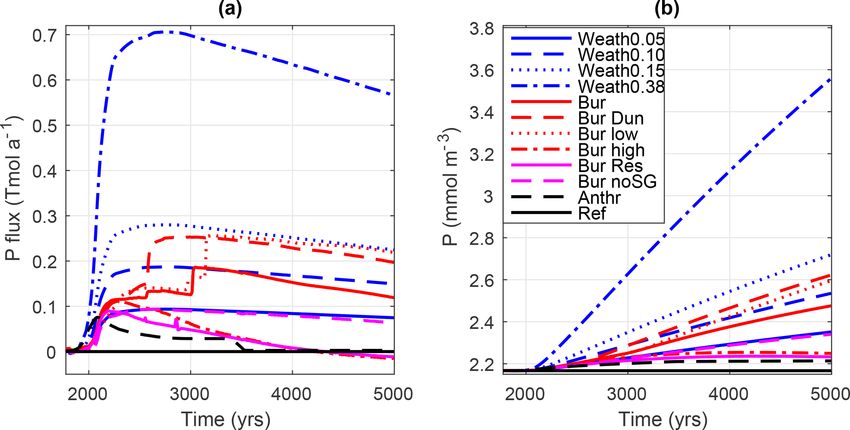
542                                                                                   T. P. Kemena et al.: Ocean phosphorus inventory

Table 1. Overview of simulations. P fluxes are given in TmolP a−1 . We divided all simulations into four groups indicated by different
colours. These are reference simulations (in roman) with and without anthropogenic fluxes of P; simulations with different formulations for
the burial (in italic beginning with the abbreviation “Bur”); simulations with weathering fluxes of P for different climate sensitivities (in bold
italic beginning with the abbreviation “Weath”); and simulations with different representations of the sediment (in bold). In the P weathering
simulations, only weathering anomalies were applied. The weathering flux in simulation Anthr is variable over time (Fig. 2a). In the P burial
simulations, a constant P weathering flux (WP,0 ) balances P burial (BURP ) during the spin-up simulations. The pre-industrial P inventory is
identical in all simulations. More detailed information can be found in the text.

   Simulations                             Abbreviation     Fluxes                              P burial parametrization
   Reference (constant P inv.)             Ref              No                                  No burial
   Anthropogenic P input                   Anthr            Flux from Filippelli (2008)         No burial
   Burial reference                        Bur              BURP (t = 1775 years) = 0.38        rC : P (Wallmann, 2010),
                                                            WP,const = 0.38                     C burial (Flögel et al., 2011)
                                                                                                YF = 123; A = 112; r = 32 in Eq. (4)
   Burial Dunne                            Bur_Dun          BURP (t = 1775 years) = 0.25        rC : P (Wallmann, 2010),
                                                            WP,const = 0.25                     C burial (Dunne et al., 2007)
   Low burial estimate                     Bur_low          BURP (t = 1775 years) = 0.21        Burial configuration but with
                                                            WP,const = 0.21                     YF = 100.5; A = 90; r = 38 in Eq. (4)
   High burial estimate                    Bur_high         BURP (t = 1775 years) = 0.60        Burial configuration but with
                                                            WP,const = 0.60                     YF = 167; A = 108.5; r = 29.5 in Eq. (4)
   Burial without subgrid bathymetry       Bur_noSG         BURP (t = 1775 years) = 0.09        Burial configuration but without subgrid
                                                            WP,const = 0.09                     bathymetry
   Burial with restricted reservoir        Bur_res          BURP (t = 1775 years) = 0.41        Burial configuration but with
                                                            WP,const = 0.41                     113 µmolP cm−2 reservoir
   Weathering                              Weath0.05        WP,0 = 0.05                         No burial
   Weathering                              Weath0.10        WP,0 = 0.10                         No burial
   Weathering                              Weath0.15        WP,0 = 0.15                         No burial
   Weathering                              Weath0.38        WP,0 = 0.38                         No burial

release from organic matter and, eventually, a net release of              larger in slope and shelf regions compared to the deep ocean
P from the sediment (BENP > RRP , in Eq. 1).                               (see Eq. 3b, c).
   Burial fluxes of P were applied in the simulations Bur,                    We examined the sensitivity of P burial to the uncer-
Bur_Dun, Bur_low, Bur_high, Bur_noSG and Bur_res. The                      tainty of the parameters in Eq. (4), describing the carbon-to-
default Bur model configuration uses Eq. (3) (Flögel et al.,               phosphorus regeneration ratio rC : P . Given means and stan-
2011) and the subgrid-scale bathymetry. Uncertainties in                   dard deviations for the parameters YF = 123±24, A = 112±
benthic P burial were examined by modifying this default                   24 and r = 32 ± 19 and assuming a Gaussian distribution,
model configuration.                                                       100 000 independent coefficient combinations were assem-
   In the Bur_Dun simulation (i.e. burial parameterization                 bled to calculate offline a range of global P burial estimates.
from Dunne et al., 2007), BURC was calculated using Eq. (5)                For the offline calculation, pre-industrial fields of O2 and
with RRC in mmol C m−2 d−1 (Dunne et al. 2007):                            RRC were extracted from the simulation Bur with a tem-
                "                      #                                   poral resolution fine enough to resolve seasonal variations
                           0.53 · RR2C                                     in the data. Global P burial varied between 0.21 TmolP a−1
BURC = RRC · 0.013 +                     ,                (5)
                          (c + RRC )2                                      (Bur_low) and 0.60 TmolP a−1 (Bur_high) for a confidence
                                                                           interval of 90 % (coefficients are shown in Table 1). Individ-
where c = 7 mmol C m−2 d−1 . This parameterization leads to                ual spin-ups were performed for the Bur_low and Bur_high
high (low) organic C burial rates for high (low) organic C rain            simulations to check that the offline calculated P burial cor-
rates. This formulation is different from the standard formu-              responded to the online values from the spin-up. Only minor
lation of burial in Eq. (3b, c), where burial depends on the C             differences between the O2 fields of the Bur spin-up and the
rain rates and in addition on the water depth. In the standard             spin-ups for Bur_low and Bur_high simulations were noted
formulation, C burial is by definition 1 order of magnitude

Earth Syst. Dynam., 10, 539–553, 2019                                                           www.earth-syst-dynam.net/10/539/2019/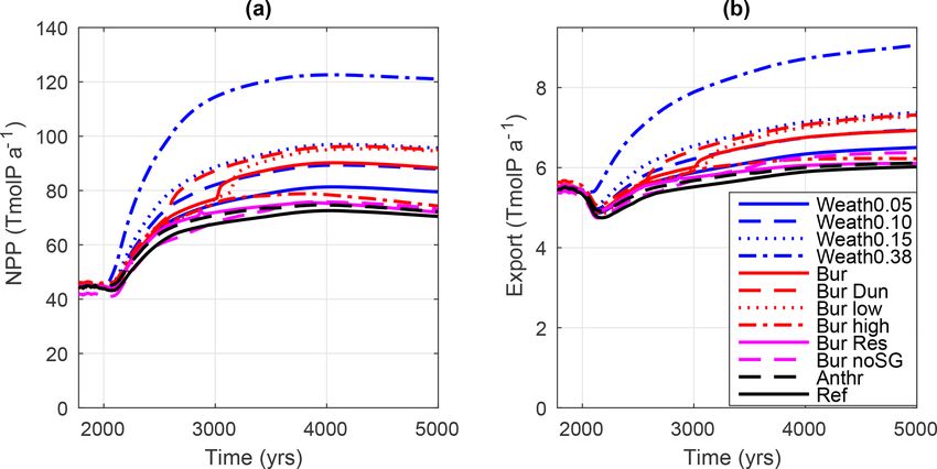
T. P. Kemena et al.: Ocean phosphorus inventory                                                                              543

(not shown), which implies negligible errors in the offline       2.4   Weathering experiments
calculation of the pre-industrial global P burial.
                                                                  Uncertainties in the ocean P inventory due to weathering pro-
   For the Bur_noSG simulation (i.e. without subgrid-scale
                                                                  cesses and anthropogenic fluxes of P were examined with the
parameterization), P fluxes at the sediment–ocean inter-
                                                                  model simulations Anthr, Weath0.05, Weath0.10, Weath0.15
face were calculated using the coarser standard model
                                                                  and Weath0.38.
bathymetry, which barely reproduces the global coverage of
                                                                    In simulations Weath0.05, Weath0.10, Weath0.15 and
shelf areas (compare hypsometries in Fig. S1 in the Supple-
                                                                  Weath0.38 (i.e. the number represents the pre-industrial
ment). This does not affect other processes like circulation,
                                                                  weathering flux), the global weathering flux of P to the ocean
advection or mixing.
                                                                  (WP ) was parameterized in terms of an anomaly relative to a
   The implemented transfer functions (Eqs. 2 and 4) assume
                                                                  pre-industrial P weathering flux (WP,0 ) according to Eq. (8).
unlimited local reservoirs of sedimentary P, meaning that the
cumulative release of P may exceed the local inventory of         WP = WP,0 · (f (NPP, SAT) − 1)                              (8)
P in the sediment if the benthic release is sustained over
a longer period of time. In the Bur_res simulation (i.e. re-      The weathering function f is given in Eq. (9). Values of
stricted release or P reservoir), we tested the impact of this    WP,0 are given in Table 1 and derived below. The chosen
simplification by applying sediment inventory restrictions to     anomaly approach assumes that, at steady state, WP,0 is bal-
sediment P release. In accordance with Flögel et al. (2011),      anced by a respective global burial flux and hence can be
release of P from the deeper ocean (> 1000 m) cannot exceed       neglected during the spin-up. In these simulations, no ben-
the rain rate of organic P to the sediment. For the continental   thic P burial was applied, and for pre-industrial conditions
shelf and slope, an upper limit sediment P inventory was cal-     the weathering function f (NPP,SAT) equals 1, and hence
culated based on the following assumptions. We assume that        WP equals 0 TmolP a−1 . The dynamic weathering function f
the top 10 cm of the sediment column are mixed by organ-          (Eq. 9) was adopted from Niemeyer et al. (2017) and is orig-
isms and are hence regarded as the active surface layer that      inally based on an equation from Lenton and Britton (2006)
is in contact with the overlying bottom water. Considering        for carbonate and silicate weathering. Following Niemeyer
a mean porosity of 0.8 and a mean density of dry particles        et al. (2017), we assumed that the release of P is proportional
of 2.5 g cm−3 , the mass of solids in this layer is 5 g cm−2      to the chemical weathering of silicates and carbonates on a
(Burwicz et al., 2011). The mean concentration of total P in      global scale. Equation (9) describes the sensitivity of terres-
continental shelf and slope sediments is 0.07 wt %, equal to      trial weathering to the change of global terrestrial net primary
22.6 µmol g−1 (Baturin, 2007). Together, these assumptions        production (NPP) and global mean surface air temperature
convert to a maximum local inventory of total solid P in the      (SAT):
active surface layer of RESP,max = 113 µmol cm−2 (Eq. 6a).
We assume that shelf and slope sediments can release up to        f =0.25 + 0.75 · (NPP/NPP0 )
100 % of the total solid P under low-oxygen conditions. The             · (1 + 0.087 (SAT − SAT0 )) ,                         (9)
local P inventory (RESP ) can be fully replenished by P sup-
ply from the water column and any excess P is assumed to be       with NPP0 and SAT0 being the respective pre-industrial val-
permanently buried:                                               ues. Increasing SAT and NPP led to enhanced weathering.
                                                                 The upper estimate of WP,0 in Weath0.38 was inferred from
  RESP ∈ R|0 ≥ RESP ≥ RESP,max                             (6a)   the P burial reference simulation Bur, assuming that the
1RESP                                                             global integral of burial is compensated by the pre-industrial
          = RRP − BENP .                                   (6b)   global weathering flux (i.e. the global marine P inventory is
   1t
                                                                  in steady state). With the simulations Weath0.05, Weath0.10,
   Local values of RESP adjust during the spin-up according       Weath0.15, and Weath0.38, we explored the range of WP,0
to the environmental conditions. Our pragmatic sediment in-       estimates as derived from observational studies, which range
ventory approach most likely overestimates the upper limit        from 0.05 to 0.30 TmolP a−1 (see Fig. 1, Benitez-Nelson,
of P that can be released from the sediments. For example,        2000; Compton et al., 2000; Ruttenberg, 2003). These studies
under low O2 conditions, part of the releasable or reactive       give a range of total P fluxes to the oceans, which are higher
P is transformed into authigenic P and permanently buried         than derived from dissolved inorganic P fluxes shown already
(Filippelli, 2001).                                               in previous studies (e.g. Martin and Meybeck, 1979; Rao and
   All Bur experiments applied a constant global weathering       Berner, 1993) and in the Global News Model (Seitzinger et
flux (WP,const ) as established during the respective spin-up     al., 2005). A small amount of fluvial P is delivered to the
run (see Table 1 for values of WP,const for the different Bur     ocean as dissolved inorganic P, but the majority (90 %) is
experiments).                                                     particulate (inorganic and organic) P (Compton et al., 2000).
                                                                  The fast transformations between dissolved and particulate P
WP = WP,const                                              (7)
                                                                  in rivers (seconds to hours) (Withers and Jarvie, 2008) sug-
                                                                  gest a much higher amount of P that is available for marine

www.earth-syst-dynam.net/10/539/2019/                                                 Earth Syst. Dynam., 10, 539–553, 2019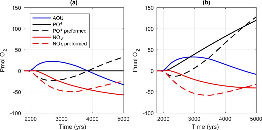
544                                                                                T. P. Kemena et al.: Ocean phosphorus inventory

Figure 1. Globally integrated pre-industrial P weathering fluxes in
                                                                         Figure 2. (a) Globally integrated flux of P in Tmol a−1 to the ocean
TmolP a−1 from field studies (red) and the range of pre-industrial P
                                                                         and (b) globally averaged phosphate concentration in mmol m−3 .
weathering fluxes covered by all simulations (blue with bars indicat-
                                                                         Simulation descriptions can be found in Table 1.
ing the range; see WP,0 in Table 1). Estimates from field studies are
based on literature values for global fluvial fluxes of bioavailable P
and the error bars denote upper and lower limits of these estimates.
                                                                         undergo a similar climate development. Maximum CO2 con-
                                                                         centrations of 2200 ppmv were reached in the year 2250 and
organisms than derived from dissolved inorganic P concen-                then declined to 1100 ppmv by the year 5000, comparable to
trations. A large amount of bioavailable P in rivers is present          results from Clark et al. (2016).
as loosely sorbed and iron-bound P. Estimates of bioavail-
able P are given in Fig. 1 (Benitez-Nelson, 2000; Compton                3.1   Fluvial P fluxes: weathering and anthropogenic
et al., 2000; Ruttenberg, 2003), which are much higher than
the estimates for dissolved inorganic P (0.018 TmolP a−1                 Largest uncertainties in the P inventory are related to the
from Seitzinger et al., 2005, or 0.03 TmolP a−1 from Filip-              large range of P weathering fluxes (Fig. 2, blue curves). Up-
pelli, 2002). Taking into account only fluxes of dissolved in-           per and lower estimates of P weathering fluxes differ by a fac-
organic P would strongly underestimate the effect of weath-              tor of 6 (Fig. 2a, blue lines). In our weathering simulations,
ering fluxes as a P source to the ocean. The weathering                  weathering anomalies depend linearly on the pre-industrial
parametrization (Eq. 9) was used to scale pre-industrial flu-            weathering flux (WP,0 ) estimate (see Eq. 8) because the cli-
vial fluxes of bioavailable P that is delivered in UVic to the           mate development is essentially equal across the simulations.
ocean as dissolved inorganic P. In the model, no distinction             Therefore, the choice of WP,0 (Fig. 1a) is a major source of
was made between particular and dissolved fluvial fluxes of              uncertainty for projected future land–ocean P fluxes.
P.                                                                          Weathering fluxes increased from the pre-industrial value
   Uncertainties to other weathering parameterizations were              by a factor of 2.5 until the year 5000 for atmospheric CO2
not investigated in this study. Our parameterization predicts            concentrations of 1100 ppmv. This is comparable with the
similar weathering rates to other weathering formulations                2- to 4-fold increase in weathering fluxes estimated during
(Meissner et al., 2012, their Fig. 6a). Since weathering is              OAE 2 approximately 91 Myr ago (Pogge von Strandmann
calculated on a global scale, we cannot study the effects of             et al., 2013) when atmospheric CO2 concentrations increased
regional lithology and soil shielding on weathered P (Hart-              to about 1000 ppmv (Damsté et al., 2008).
mann et al., 2014). UVic does not resolve the P cycle in the                In contrast to weathering-induced P input, anthropogenic
rivers, which is an active field for scientific research (Beusen         P fluxes (Filippelli, 2008) influence the global marine P in-
et al., 2016; Harrison et al., 2019).                                    ventory only in the near future (Fig. 2a, dashed black line).
   Finally, global anthropogenic P fluxes from fertilization,            A decline in anthropogenic P fluxes after the year 2100 is
soil loss due to deforestation and sewage as projected by Fil-           expected due to the depletion of the easily reachable phos-
ippelli (2008) were prescribed in the simulation Anthr (an-              phorite mining reserves (Filippelli, 2008).
thropogenic).
                                                                         3.2   Sediment fluxes: parameterizations, subgrid
                                                                               bathymetry, sediment reservoir
3   Uncertainties in the phosphorus inventory
                                                                         The release of P from the sediment is strongly dependent on
The large range of projected global P fluxes to the ocean from           the O2 concentration in the water above the sediments (Wall-
sediments or weathering (Fig. 2a) leads to uncertainties in              mann, 2003; Flögel et al., 2011). Climate warming reduces
future P inventories by up to 60 % of the present-day value              O2 solubility and ventilation of the ocean, which decreases
until the year 5000 (Fig. 2b). All simulations show negligi-             the global O2 content (more details in Sect. 4). The general
ble differences in atmospheric CO2 concentrations and hence              decrease in ocean O2 content may therefore cause preferen-

Earth Syst. Dynam., 10, 539–553, 2019                                                        www.earth-syst-dynam.net/10/539/2019/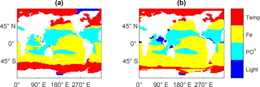
T. P. Kemena et al.: Ocean phosphorus inventory                                                                                     545

                                                                    Figure 4. Globally integrated pre-industrial rain rate of particulate
                                                                    organic carbon (RRC ) to the seafloor in TmolC a−1 from published
                                                                    studies (red) and for UVic model simulations (blue) between 0 to
                                                                    2000 m water depth (dark blue) and below 2000 m (light blue). The
Figure 3. Globally integrated pre-industrial P burial fluxes in     simulation Bur is representative for all UVic model simulations ex-
TmolP a−1 from field studies (red) and for UVic model simulations   cept Bur_noSG.
in the year 1775 (blue). Description of the model simulations can
be found in Table 1.
                                                                       Simulated pre-industrial RRC increased significantly from
                                                                    180 to 1040 TgC a−1 on the shelf and globally from 900
tial release of P from marine sediments. Differences in sed-        to 1500 TgC a−1 compared to simulations without subgrid
iment P fluxes in our simulations are related to uncertainties      bathymetry. Pre-industrial RRC with subgrid bathymetry
in the parameterization of the transfer function (Fig. 2, red       agrees better to estimates by Bohlen et al. (2012) (Table 2)
lines, −0.01 to 0.22 TmolP a−1 by the year 5000), to differ-        and to other field data studies reporting a range from 900 to
ent representations of the bathymetry (Fig. 2, dashed purple        2300 TgC a−1 (Fig. 4) (Muller-Karger et al., 2005; Burdige,
line: 0.06 (without subgrid) and 0.12 (Bur) TmolP a−1 ) and         2007; Dunne et al., 2007; Bohlen et al., 2012).
to the way sediment P reservoirs in the sediment are repre-            In summary, subgrid bathymetry leads to a substantial im-
sented (Fig. 2, solid purple line: −0.01 (limited reservoir)        provement of the representation of RRC to the sediment.
and 0.12 (unlimited reservoir, Bur) TmolP a−1 ).                    More realistic benthic fluxes of P could be also attained by
   The global P burial of approximately 0.2 TmolP a−1               adjusting parameters for rC : P (Eq. 4) or by using the func-
(Fig. 3) (Filippelli and Delaney, 1996; Benitez-Nelson, 2000;       tion of Dunne et al. (2007) to calculate BURC (Eq. 5). The
Ruttenberg, 2003) is relatively well reproduced by simula-          implementation of a finite P reservoir in the sediment has a
tions Bur_low and Bur_Dun. The simulation with the stan-            substantial impact on the transient development of the global
dard UVic bathymetry (Bur_noSG) underestimates P burial             P inventory on millennial timescales. This is an important im-
by 60 %, while simulations Bur_high, Bur and Bur_res over-          provement relative to earlier work and should be considered
estimate P burial by 180 %, 90 % and 80 % with respect to es-       in future studies.
timates based on observations. The transient response of the
P release to O2 was stronger for simulations with low burial,
and vice versa (Fig. 2), except for simulation Bur_res. In          4   Ocean deoxygenation and suboxia
Bur_res, a significant reduction in the transient P release oc-
                                                                    Climate change influences ocean oxygen content by changes
curred due to the implementation of a finite P reservoir, with
                                                                    in circulation, ocean temperature and the degradation of or-
net global P loss due to enhanced burial at the end of the sim-
                                                                    ganic matter. In warming surface waters, the solubility of
ulation. In the year 5000, global P concentrations increased
                                                                    O2 decreases along with an increase in stratification, which
in Bur_res by only 0.06 mmolP m−3 compared to the global
                                                                    together cause the deeper ocean to becomes less ventilated
mean pre-industrial concentration of 2.17 mmolP m−3 . This
                                                                    (Bopp et al., 2002; Matear and Hirst, 2003; Oschlies et al.,
is 6-fold smaller than the increase of 0.36 mmolP m−3 in sim-
                                                                    2018; Shaffer et al., 2009). Changes in export production
ulation Bur with an assumed unlimited P reservoir. The small
                                                                    and the degradation of organic matter in the ocean interior
increase in the oceanic P inventory in Bur_res can be ex-
                                                                    also affect O2 content. In the following, we analyse the im-
plained by the reduction in P sediment inventory rather than
                                                                    pact of different ocean P inventories on ocean deoxygenation
by changes in the rain rate of particulate organic matter to
                                                                    and suboxia (Fig. 5). For a more detailed analysis, we com-
the sediment (RRC ). In Bur, a rapid increase in the benthic
                                                                    pare Weath0.15 to the Ref simulation. In the Weath0.15 sim-
P release appeared in areas where the water turned suboxic
                                                                    ulation, the assumed pre-industrial weathering flux compares
and thus drove a positive benthic feedback between P release,
                                                                    well to estimates from observations (Fig. 1).
productivity and deoxygenation (Fig. 2a). A limited supply
                                                                       In the Ref simulation, global suboxic volume increased
of P from the sediment (Bur_Res) dampens this feedback.
                                                                    due to climate change from 0.3 to 1 % until the year 5000
                                                                    (similar to Schmittner et al., 2008), and the suboxic sediment

www.earth-syst-dynam.net/10/539/2019/                                                    Earth Syst. Dynam., 10, 539–553, 2019
546 T. P. Kemena et al.: Ocean phosphorus inventory
Table 2. Rain rate of particulate organic carbon (RRC ) to the seafloor for the shelf, slope and deep-sea areas from the observational estimate
by Bohlen et al. (2012) and for the UVic model simulation (Bur) with and without subgrid bathymetry. Pre-industrial RRC shows no
significant differences among all model simulations (expect for simulation Bur_noSG).
Bohlen (2012) UVic model with UVic model without
subgrid bath. subgrid bath.
(simulation Bur) (simulation Bur_noSG)
Depth RRC RRC Area RRC RRC Area RRC RRC Area
(m) (TgC a−1 ) (%) (%) (TgC a−1 ) (%) (%) (TgC a−1 ) (%) (%)
Shelf 0–200 1056 60 6 1039 70 6.5 179 28 2.3
Slope 200–2000 393 22 10 205 14 11.7 219 34 13.3
Deep sea > 2000 312 18 84 235 16 81.9 238 37 84.6
Sum 1761 1479 637
Figure 5. Globally integrated (a) suboxic volume in percentage of Figure 6. Globally integrated (a) ocean net primary production
total ocean volume and (b) suboxic sediment surface area in per- (NPP) in TmolP a−1 and (b) export of organic P below the 130 m
centage of total sediment surface area. Water is designated as sub- depth level in TmolP a−1 . Simulation descriptions can be found in
oxic for oxygen concentrations below 5 mmolO2 m−3 . Simulation Table 1.
descriptions can be found in Table 1.
ally integrated signal in comparison to the extent of suboxia,
which is a consequence of more local processes.
area increased from 0.06 to 0.23 % (Fig. 5, black line). In the
Weath0.15 simulation, the increase in suboxic volume (sub- 4.1 Enhanced biological pump
oxic sediment area) was more than 2 (3) times higher than for
the Ref simulation. The expansion of suboxic sediment areas The biological carbon pump can be summarized as the sup-
was also enhanced for simulations with benthic fluxes, which ply of biologically sequestered CO2 to the deep ocean. In
could be related to regional feedbacks between increasing the euphotic zone, phytoplankton and diazotrophs take up
marine productivity, decreasing oxygen and enhanced sedi- CO2 , a process that is intensified by elevated PO4 concen-
mentary P release (Tsandev and Slomp, 2009). The explic- trations in the surface ocean (Fig. 6a). Part of the organic
itly simulated finite sedimentary P reservoir in simulation matter sinks out of the euphotic zone (Fig. 6b) to the ocean
Bur_res places an upper limit to the benthic release of P interior, where it is respired using O2 . It is therefore P supply
and dampens these regional feedbacks, resulting in a weaker to the surface waters that explains the differences in deoxy-
spreading of suboxic waters by only 17 % compared to the genation between the simulations. Circulation changes could
Ref simulation. also affect the supply of O2 to the ocean interior. However,
In the following sections, we show how the expansion of no significant differences in climate and circulation appeared
suboxia is related to net primary production (NPP) in the among the simulations, and therefore the global-warming-
ocean, the export of organic matter (Sect. 4.1) and nitrogen induced circulation changes affected all simulations in the
limitation (Sect. 4.2). Finally, we show how changes in O2 same way.
solubility and utilization vary over time and affect the global In the Ref simulation, NPP (Fig. 6a, black line) increased
O2 inventory (Sect. 4.3). The latter approach gives another from 45 to 70 TmolP a−1 (57 to 89 GtC a−1 ) by the end of the
perspective because changes in O2 inventories are a glob- simulation. In Weath0.15, enhanced P supply to the ocean
Earth Syst. Dynam., 10, 539–553, 2019 www.earth-syst-dynam.net/10/539/2019/T. P. Kemena et al.: Ocean phosphorus inventory 547
Figure 8. Spatial distribution of the most limiting factors for growth
of diazotrophs for (a) the pre-industrial case and (b) simulation
year 5000 for Weath0.15. Limitation of iron (Fe) and phosphate
(PO4 ) is based on Monod kinetics so that the limitation factors vary
Figure 7. Globally averaged (a) N2 fixation in mmolN m−3 a−1 between 0 and 1. The light limitation factor also varies between 0
and (b) NO− −3
3 concentration in mmolN m . Simulation descrip- and 1. In the model, diazotrophs only grow at temperatures higher
tions can be found in Table 1. than 15.7 ◦ C. For temperatures above 15.7 ◦ C, diazotroph growth
depends on the equation exp(T /15.7 ◦ C)−2.61. Diazotroph growth
is not limited by nitrate availability in the model. A more detailed
led to a doubling of NPP compared to the Ref simulation. description of diazotroph growth and iron limitation can be found
The P inventory increased continuously, but NPP did not fol- in Keller et al. (2012) and Nickelsen et al. (2015).
low this trend and instead peaked in the year 4000. In the
year 5000, all simulations, excluding Weath0.38, showed a
similar response of NPP to the P addition, with an increase ture being zero below 15 ◦ C, is slower relative to non-fixing
in NPP of 19 TmolP a−1 (relative to the Ref simulation) per phytoplankton. These characteristics allow them to succeed
10 % increase in P inventory. In Weath0.38, the response was in warm, low-N and high-P environments that receive suf-
weaker and NPP increased by 8 TmolP a−1 per 10 % rise in ficient iron. In all simulations, N2 fixation was stimulated
the P concentration. P is less effectively utilized in simula- by the addition of P to the ocean and was sensitive to rapid
tions with large oceanic P inventories. Higher ocean tem- changes in the supply of P (compare Figs. 7a and 2a). How-
peratures enhanced remineralization of organic matter in the ever, N2 fixers (Fig. 7a) were not able to use the extra P sup-
shallower ocean so that the overall export to NPP ratio de- ply in polar and iron-limited regions where low temperatures
creased from its pre-industrial value of 0.12 to an average and iron limitation, respectively, inhibit their growth (Fig. 8).
value among all simulations of 0.08 by the year 5000. This This led to a substantial amount of excess phosphate in the
is because despite the warming-driven enhanced remineral- surface waters of these regions (Fig. S2). Because N2 fix-
ization, the warming-driven intensification of ocean stratifi- ers were not able to balance the loss by denitrification, ni-
cation leads to a decline in supply of nutrients to the surface trate decreased globally by 4 mmol N m−3 by the year 5000
layer and reduced export production, in line with earlier stud- (Fig. 7b). The loss in nitrate led to a decrease in globally av-
ies (e.g. Bopp et al., 2013; Landolfi et al., 2017). eraged N-to-P ratios. In the Ref simulation, N : P decreased
To summarize, NPP and export of organic matter are sen- from 14 to 12, and for the Weath0.15 simulation it decreased
sitive to P addition. However, the proposed positive feedback to 10, which contributed further to a N-limiting ocean. The
between P, NPP, export of organic matter and deoxygenation nitrogen cycle was not able to recover from the decrease in
was limited in our simulations due to a negative feedback N : P ratio with respect to pre-industrial values. We acknowl-
related to nitrate availability. This is shown and explored in edge that in the current study we did not account for potential
the following section. We acknowledge that accounting for future changes in iron concentrations (from atmospheric de-
P burial in weathering simulations may limit the P increase. position, shelf inputs) and that the lack of a fully prognostic
However, the effect of P burial has been shown to be small iron model may lead to a different sensitivity of the response
relative to the increase in benthic release of P due to the feed- of diazotrophs. Similarly, we did not account for the abil-
back involving redox-sensitive benthic P fluxes associated ity of phytoplankton to adapt to changing N : P ratios, which
with the expansion of OMZ (Niemeyer et al. 2017, Fig. S1). may affect marine biological productivity and in turn deoxy-
genation. These would require further studies.
4.2 Nitrogen limitation
4.3 Temporal variations of deoxygenation
At the end of the spin-up, the N sink by denitrification and
the N source by N2 fixation were balanced. In the Ref simula- Anomalies in circulation, ocean temperature and reminer-
tion, climate warming enlarged the oxygen minimum zones, alization of organic matter affect oceanic O2 levels in a
which enhanced denitrification in the tropics (not shown). In climate-warming scenario. In the Ref simulation, the O2 in-
our model, diazotrophs are limited by P and Fe and are not ventory (Fig. 9a) decreased by 60 Pmol O2 by the year 3000
limited by N. Their growth rate, which depends on tempera- and then reached present-day values again by the year 5000.
www.earth-syst-dynam.net/10/539/2019/ Earth Syst. Dynam., 10, 539–553, 2019548 T. P. Kemena et al.: Ocean phosphorus inventory
Figure 10. Anomalies of globally integrated AOU (blue line),
PO3− 3−
4 (solid black line), preformed PO4 (dashed black line), NO3
−
(solid red line) and preformed NO− 3 (dashed red line) expressed
in Pmol O2 equivalents using constant elemental ratios (O : N = 10
and O : P = 160) for the (a) Ref simulation and the (b) Weath0.15
simulation. Preformed nutrients are calculated as the difference be-
tween remineralized and total nutrient content. The calculations as-
sume that all ocean water leaves the surface layer saturated in O2 .
Figure 9. Anomalies of globally integrated (a) O2 content, (b) ap-
parent oxygen utilization (AOU) and (c) oxygen saturation (O2, sat ) among all simulations and contributed to a re-oxygenation
in Pmol O2 . Simulation descriptions can be found in Table 1. of the ocean. For simulations with larger P inventories, the
AOU had a larger positive offset to the Ref simulation.
In a model with constant stoichiometry for elemental ex-
In Weath0.15, weathered P enhanced deoxygenation and led change by biological processes, anomalies in AOU (Fig. 10,
to a greater decrease in O2 than in the Ref simulation. The blue lines) can be explained by the difference between to-
O2 decrease was up to 70 Pmol by the year 3300 and O2 still tal integrated nutrients (Fig. 10, solid red and black lines as
showed a negative anomaly of 24 Pmol O2 by the year 5000. anomalies) and preformed nutrients (Fig. 10, dashed red and
Global anomalies in O2 were due to changes of the apparent black lines as anomalies). Preformed nutrients correspond to
oxygen utilization (AOU; Fig. 9b) and the O2 saturation level the fraction that leaves the surface ocean unutilized by phyto-
(Fig. 9c). AOU is calculated from the difference between the plankton (Ito and Follows, 2005). For example, in the South-
O2 saturation concentration and the in situ O2 concentration ern Ocean, a large fraction of nutrients that leaves the surface
assuming that all ocean water leaves the surface layer satu- is preformed. The fraction of utilized and preformed nutri-
rated in O2 . The calculation of AOU is in general biased to- ents can change during a transient simulation and could af-
wards higher values, because in polar regions the water that fect the oxygen state of the ocean.
is subducted and mixed into the deep water is undersaturated In the Ref simulation (Fig. 10a), the anomaly of preformed
with respect to O2 as a result of reduced air–sea gas transfer dissolved inorganic P was directly inverse to the anomaly of
by sea ice (Ito et al., 2004). In UVic, this leads to an overes- AOU because the oceanic P Inventory was conserved in this
timation of AOU by 30 % (Duteil et al., 2013). Sea ice cover simulation. Until the year 2200, changes in circulation and
reduces in a warming ocean that leads to an underestima- climate are the main cause for the reduction in preformed N
tion of the AOU anomaly in Fig. 9c. Changes in O2 satura- and P in the Ref simulation since global N and P inventories
tion were similar across the model simulations and lagged were almost constant in this time period (Fig. 9a, solid red
behinds surface ocean temperature changes. The circulation and black line). During continuous and intense ocean warm-
and ventilation of the ocean were similar in the model sim- ing, a weakening of the meridional overturning (not shown)
ulations because differences in surface temperatures were reduced ocean ventilation. The meridional overturning max-
negligible and the atmospheric forcing of the ocean circu- imum decreased from 17 Sv (pre-industrial) to 11 Sv in the
lation was identical so that differences in AOU depended al- year 2200. The continuous warming and stratification of the
most only on biological O2 consumption and AOU anomalies ocean reduces the supply of nutrients to the surface layer
were directly yet inversely related to the changes in O2 lev- from the deep ocean. This is consistent with a reduction of
els. Hence, biological consumption explained variations in the export of organic matter until the year 2200 (Fig. 6b). The
O2 content among the different model simulations (compare balance between exported P out of the surface ocean and sup-
Fig. 9a and b). Increasing O2 utilization contributed to the de- plied P controls changes in AOU. We suggest that a weaker
crease of O2 levels until the year 3000. Thereafter, a distinct overturning increased the residence time of water and nu-
negative trend in AOU with a similar slope was observed trients in the surface ocean. Nutrients staying longer in the
Earth Syst. Dynam., 10, 539–553, 2019 www.earth-syst-dynam.net/10/539/2019/T. P. Kemena et al.: Ocean phosphorus inventory 549
euphotic zone are more likely to be biologically consumed. the local sedimentary P inventory can greatly overestimate
This implies more efficient utilization of nutrients and hence the release of benthic P on long timescales. In the UVic
the reduction in preformed nutrients and an increase in AOU. model, the application of finite benthic P inventories limited
Enhanced suboxia after the year 2200 drove excess den- the benthic release significantly. Under low-oxygen condi-
itrification and a decline in nitrate (Fig. 10a, solid red line) tions, sediments were P depleted already after a few years
in the Ref simulation. The decline in nitrate could explain to decades. In our simulation, this resulted in an increase
the negative trend in AOU anomalies (Fig. 10a, solid blue in the global oceanic P inventory by just 3 % (Fig. 2, solid
line) and therefore a negative feedback on the global deoxy- magenta line). This could imply that benthic release of P is
genation. In the year 2200, overturning had started to recover actually negligible in comparison to the weathering fluxes
quickly and increased to 21 Sv in the year 3000 (+24 % rela- of P, but the UVic model does not resolve coastal processes
tive to pre-industrial values), leading to faster overturning of such as the deposition of reactive particulate P from rivers
organic matter in the surface ocean and a decrease in global on the continental shelves and its dissolution and release to
AOU. This suggests that the slight increase in export by 5 % the water column. For a more realistic comparison of benthic
(relative to pre-industrial values) was not strong enough to and fluvial P fluxes, a more detailed representation of coastal
compensate for the 24 % faster overturning, which reduced processes would be necessary to simulate deposition and re-
the residence time of nutrients in the surface ocean. lease of fluvial P from the sediments at the shelf. However,
P addition in the Weath0.15 simulation stimulated N2 fixa- we can conclude that the actual local inventories of P are too
tion by diazotrophs and counteracted N loss by denitrification small to sustain a positive benthic P feedback over several
(Fig. 10b, solid red line). This led to an increase in N inven- millennia. Further, we find that a more realistic bathymetry
tory by 17 Pmol O2 equivalents compared to the Ref simula- substantially improves the simulated rain rate of particular
tion. Furthermore, the high availability of P seems to reduce organic carbon to the sediment (Table 2), particularly on the
preformed N by 6 Pmol O2 equivalents. Both explain the dif- shelf, which most models do not resolve. Anthropogenic P
ference in AOU between Weath0.15 and Ref of 24 Pmol O2 fluxes increased the global P inventory by just 2 % (Fig. 2,
at the end of the simulation (Fig. 9b). However, denitrifica- dashed black line). In summary, considering the weathering
tion still exceeded N2 fixation, which led to low levels of parameters closest to the present day, the model formulation
nitrate. From the year 5000, approximately all of the added with limited P reservoir and anthropogenic fluxes from Fil-
P in the Weath0.15 simulation remained unused by phyto- ippelli (2008), assuming a linear combination of all P inputs,
plankton, left at the surface ocean as preformed P, and was we find a +30 % increase in the total global ocean P inven-
afterwards stored in the deep ocean. Phytoplankton was un- tory by the year 5000. This seems to be surprisingly high,
able to utilize the extra P because it was limited by nitrate. but several studies indicate that changes in past climate could
Diazotrophs could not counteract the lack of N due to iron also have been accompanied by substantial changes in the P
limitation and low surface temperatures in the polar oceans. inventory but at a much lower pace (Planavsky et al., 2010;
The denitrification feedback driven by the spread of suboxic Monteiro et al., 2012; Wallmann, 2014). In this simple ad-
conditions in the tropics had reduced further the N availabil- dition of the P inventories, we cannot account for feedbacks
ity for phytoplankton and limited the effect of P addition on that might become apparent in a fully coupled model. For
the global oxygen level. such high P inventories, we would expect larger suboxia and
therefore more P release from sediments and at the same time
a stronger export of organic P and increased P burial.
5 Discussion and conclusions The increased P inventory (Fig. 2b) promotes deoxygena-
tion (Fig. 5) and expansion of suboxia, but it also causes a
In this study, we compare simulations with different bio- net loss of nitrate, which appears to further limit the full
geochemical P settings but with virtually the same ocean utilization of P by phytoplankton in our simulations. Wall-
circulation. We find that the O2 and P inventories are very mann (2003), using a box model, already recognized that for
sensitive to the weathering and benthic P flux parameter- a eutrophic ocean, nitrate might ultimately limit marine pro-
izations tested in our model. Large uncertainties (Fig. 2, ductivity. As a consequence, large amounts of P leave the
blue lines) derive from the poorly constrained estimate for surface ocean as preformed P (Fig. 10b) with no further im-
the pre-industrial P weathering flux that ranges from 0.05 pact on O2 levels in the ocean interior. Low N : P ratios are
to 0.30 Tmol P a−1 (Benitez-Nelson, 2000; Compton et al., thought to give N2 fixers a competitive advantage over or-
2000; Ruttenberg, 2003). The pre-industrial weathering flux dinary phytoplankton and lead to an increase in N2 fixation
in simulation Weath0.15 (0.15 Tmol P a−1 ) is well in this (Fig. 7a). In the time period of OAE1a and OAE2, a substan-
range. In this simulation, enhanced weathering leads to an tial increase in N2 fixation was also inferred from measure-
increase in the global ocean P inventory by 25 % until the ments of sediment nitrogen isotope compositions typical for
year 5000 (Fig. 2, dotted blue line). Benthic fluxes of P were newly fixed nitrogen conditions and from high abundances
simulated using transfer functions on a subgrid bathymetry. of cyanobacteria indicated by a high 2-methylhopanoid index
Applying the transfer functions without taking into account (Kuypers et al., 2004). However, high denitrification rates re-
www.earth-syst-dynam.net/10/539/2019/ Earth Syst. Dynam., 10, 539–553, 2019550 T. P. Kemena et al.: Ocean phosphorus inventory
move nitrate from the global ocean, and in the UVic model Code and data availability. The model data and the model code
N2 fixers are not able to compensate for this loss (Fig. 7b) are available at https://data.geomar.de/thredds/catalog/open_access/
because low temperatures in polar regions and iron limita- kemena_et_al_2018_esd/catalog.html (Kemena, 2019).
tion at lower latitudes inhibit growth of diazotrophs (Fig. 8),
and a substantial amount of excess phosphate remains in the
surface waters in these regions (Fig. S2). General circulation Supplement. The supplement related to this article is available
models without a N cycle, or box models without realistic online at: https://doi.org/10.5194/esd-10-539-2019-supplement.
representation of habitats suitable for N2 fixers, would miss
this important negative feedback limiting global deoxygena-
Author contributions. All authors discussed the results and
tion. As a next step, it would be reasonable to investigate
wrote the manuscript. TPK led the writing of the manuscript and
how different parameterizations of the N cycle and a full the data analysis.
dynamic iron cycle will affect the utilization of the added
P. For example, benthic denitrification is not simulated in
the UVic model. Model simulations showed, for this cen- Competing interests. The authors declare that they have no con-
tury, that the enhanced denitrification in the water column flict of interest.
could be compensated by less benthic denitrification (Lan-
dolfi et al., 2017), which could reduce the N limitation and
therefore enhance the effect of P fluxes on the biological Acknowledgements. This study is a contribution to the Son-
pump. Sources of bioavailable Fe are still not well quanti- derforschungsbereich (SFB) 754 “Climate-Biogeochemical Interac-
fied and how these sources change under climate change is tions in the Tropical Ocean” and it was supported by the German
under debate (Hutchins and Boyd, 2016; Mahowald et al., Research Foundation through the Emmy Noether Program (inde-
2005). A more realistic representation of a dynamic iron cy- pendent junior research group ICONOX). We thank Wolfgang Ko-
cle in UVic would affect N2 fixation in many areas of the eve for his helpful and valuable comments.
global ocean (Fig. 8). Some additional model limitations are
a cause for uncertainty in our results. We considered a fixed
Redfield-ratio stoichiometry. In future deoxygenation stud- Financial support. The article processing charges for this open-
access publication were covered by a Research Centre of the
ies, an optimality-based model for nutrient uptake with vari-
Helmholtz Association.
able nutrient ratios (Pahlow et al., 2013) could be applied
to investigate how well marine organisms adapt to a chang-
ing nutrient availability in the global ocean. Sea level change Review statement. This paper was edited by Axel Kleidon and
and the implied bathymetry change were not simulated in the reviewed by two anonymous referees.
UVic model. In future projections, higher surface air tem-
peratures would lead to a rise in sea level, which increases
global coverage of shelf areas. Burial of P is more effective
on the shelf (Flögel et al., 2011), which would remove P from References
the ocean and lead to a lower marine P residence time (Bjer-
rum et al., 2006). Finally, the model does not consider a fully Archer, D.: A data driven model of the global cal-
cite lysocline, Global Biogeochem. Cy., 10, 511–526,
prognostic (vertically resolved) sediment model for C burial,
https://doi.org/10.1029/96GB01521, 1996.
which may reduce O2 consumption in water depths shallower
Battaglia, G. and Joos, F.: Hazards of decreasing marine oxy-
than 1 km. gen: the near-term and millennial-scale benefits of meeting
To conclude, climate warming leads to a larger oceanic P the Paris climate targets, Earth Syst. Dynam., 9, 797–816,
inventory mainly due to addition of P by weathering but also https://doi.org/10.5194/esd-9-797-2018, 2018.
due to the release of P from the sediment and due to anthro- Baturin, G. N.: Issue of the relationship between primary produc-
pogenic fluxes. A realistic representation of shelf bathymetry tivity of organic carbon in ocean and phosphate accumulation
improves the predicted benthic P fluxes. Transfer functions (Holocene-Late Jurassic), Lithol. Miner. Resour., 42, 318–348,
for benthic P release should consider the sedimentary P in- https://doi.org/10.1134/S0024490207040025, 2007.
ventory. However, the largest uncertainties in the projection Bauer, K. W., Zeebe, R. E., and Wortmann, U. G.: Quantifying the
of oceanic P inventory are due to poorly constrained weather- volcanic emissions which triggered Oceanic Anoxic Event 1a
and their effect on ocean acidification, Sedimentology, 64, 204–
ing fluxes of P. Although additional deoxygenation is driven
214, https://doi.org/10.1111/sed.12335, 2017.
by P addition to the ocean, the degree of deoxygenation –
Benitez-Nelson, C. R.: The biogeochemical cycling of phos-
and hence the positive redox-related feedback on benthic P phorus in marine systems, Earth. Sci. Rev., 51, 109–135,
release – is eventually limited by the availability of N and https://doi.org/10.1016/S0012-8252(00)00018-0, 2000.
the apparent inability of the modelled N2 fixation to respond Beusen, A. H. W., Bouwman, A. F., Van Beek, L. P. H., Mogollón,
to the larger P inventory. J. M., and Middelburg, J. J.: Global riverine N and P transport
to ocean increased during the 20th century despite increased re-
Earth Syst. Dynam., 10, 539–553, 2019 www.earth-syst-dynam.net/10/539/2019/You can also read