PHYSICAL REVIEW RESEARCH 2, 033237 (2020) - Physical Review Link ...
←
→
Page content transcription
If your browser does not render page correctly, please read the page content below
PHYSICAL REVIEW RESEARCH 2, 033237 (2020)

                                            One-dimensional cell motility patterns

                 Jonathan E. Ron,1 Pascale Monzo ,2 Nils C. Gauthier,2 Raphael Voituriez,3 and Nir S. Gov                      1
                     1
                       Department of Chemical and Biological Physics, Weizmann Institute of Science, 7610001, Israel
                                     2
                                       IFOM, FIRC Institute of Molecular Oncology, Milan, 20139, Italy
                3
                  Laboratoire Jean Perrin and Laboratoire de Physique Thorique de la Matire Condense, Sorbonne Universit,
                                   Tour 13-12, 5eme etage, 4 place Jussieu, 75252 Paris Cedex 05, France

                                   (Received 6 March 2020; accepted 23 July 2020; published 11 August 2020)

                 During migration, cells exhibit a rich variety of seemingly random migration patterns, which makes unraveling
              the underlying mechanisms that control cell migration a difficult challenge. For efficient migration, cells require
              a mechanism for polarization, so that traction forces are produced in the direction of motion, while adhesion
              is released to allow forward migration. To simplify the study of this process, cells have been studied when
              placed along one-dimensional tracks, where single cells exhibit both smooth and stick-slip migration modes. The
              stick-slip motility mode is characterized by protrusive motion at the cell front, coupled with a slow elongation of
              the cell, which is followed by a rapid retraction of the cell rear. In this study, we explore a minimal physical model
              that couples the force applied on the adhesion bonds to the length variations of the cell and to the traction forces
              applied by the polarized actin retrograde flow. We show that the rich spectrum of cell migration patterns emerges
              from this model as different deterministic dynamical phases. This result suggests a source for the large cell-to-
              cell variability (CCV) in cell migration patterns observed in single cells over time and within cell populations:
              fluctuations in the cellular components, such as adhesion strength or polymerization activity, can shift the cells
              from one migration mode to another, due to crossing the dynamical phase transition lines. Temporal noise is
              shown to drive random changes in the cellular polarization direction, which is enhanced during the stick-slip
              migration mode. The model contains an emergent critical length for cell polarization, whereby cells that retract
              below this length loose polarity, and are prone to making direction changes in migration. These results offer a
              new framework to explain experimental observations of migrating cells, resulting from noisy switching between
              underlying deterministic migration modes.

              DOI: 10.1103/PhysRevResearch.2.033237

                      I. INTRODUCTION                                      observed during cell migration is not understood [6], and is
                                                                           usually ascribed to the inherent noise of cellular systems [7,8].
    Eukaryote cell migration, whereby cells crawl actively over
                                                                              To simplify the study of the complex process of cell
an external substrate, is a subject of great interest for biolog-
                                                                           motility, cells can be confined to move along one-dimensional
ical processes such as development and cancer progression.
                                                                           tracks, either on flat adhesive stripes [9,10], linear grooves
Adhesion-based cell motility involves the orchestration of a
                                                                           [11] and channels [12,13], or thin fiber [14,15]. In addition
large number of cytoskeletal proteins: Typically, the cell needs
                                                                           to being a simple geometry for the study and analysis of the
to break its symmetry (polarize), and produce traction forces
                                                                           cell motion in general, such confined motion appears also
in the direction of polarization (balanced by drag or friction
                                                                           in-vivo [16], for example when cells move along axonal fibers
forces). The traction forces are mediated by adhesion between
                                                                           [17,18], or cancer invades in confined spaces between tissues
the cell and the external substrate, but these adhesions have to
                                                                           [19].
detach at the trailing end of the cell in order to allow the cell
                                                                              The experiments listed above have shown that isolated
to migrate forward. When observing freely migrating cells
                                                                           cells on one-dimensional tracks exhibit the following stereo-
(i.e., not guided by an external gradient of any kind), one is
                                                                           typical behaviors [9,10]: (i) nonmigrating and unpolarized,
often struck by the large variation in their migration patterns
                                                                           by remaining quiescent or elongating symmetrically, (ii) un-
[1–5], both for a single cell over time, and for a (seemingly
                                                                           dergoing spontaneous symmetry breaking, polarization and
identical) cell population. The origin of the large cell-to-cell
                                                                           migrating smoothly, and (iii) as in (ii) but exhibiting stick-slip
variability (CCV), or phenotypic, population heterogeneity,
                                                                           migration. The stick-slip motility mode is characterized by
                                                                           protrusive motion at the cell front, coupled with an overall
                                                                           elongation of the cell and followed by rapid retraction of
                                                                           the cell back. In both (ii) and (iii), the cell motility can be
Published by the American Physical Society under the terms of the          highly persistent, or undergo sporadic direction changes. The
Creative Commons Attribution 4.0 International license. Further            appearance of this variety of migration behaviors within a
distribution of this work must maintain attribution to the author(s)       uniform cell population, as well as the switching of cells
and the published article’s title, journal citation, and DOI.              between these modes, remains an open puzzle and is the aim

2643-1564/2020/2(3)/033237(27)                                033237-1                              Published by the American Physical Society
RON, MONZO, GAUTHIER, VOITURIEZ, AND GOV                                            PHYSICAL REVIEW RESEARCH 2, 033237 (2020)

of this work. Clearly the diversity of the migration patterns is
beyond modeling the cell motility as a simple random walk
process [4,20–22].
   We present a theoretical model that describes the cell
motility in a highly simplified, and coarse-grained manner. By
coarse-grained we mean that we do not describe the cellular
dynamics at the molecular or actin-filament scale. Never-
theless, the model contains two key, and strongly coupled,
components: a slip-bond adhesion module at the cell back and
a cellular polarization module. We find that these components
are sufficient to drive the entire spectrum of observed motility
patterns, and explain the transitions between them. Our work
therefore demonstrates how a minimal model gives rise to a
rich variety of deterministic migration patterns, as opposed
to complex motion that is purely driven by different levels
of cellular noise. In experiments, these deterministic patterns
may underlie the migration of cells, but further confounded by             FIG. 1. The simplified model. (a) Illustration of the physical
noise.                                                               model of a cell migrating along a linear track. xb and x f represent the
   The stick-slip motion is shown here to have an underlying         back and front part of the cell of the cell which are connected by an
deterministic oscillatory behavior, separated from smooth mi-        effective spring with a stiffness k. x0 is the rest length of the spring
gration by a bifurcation line. Previous treatments of stick-slip     (cell) and l is the length of the cell. v is the velocity of the actin
dynamics of cells focused on the protrusion-retraction cycles        retrograde flow which is assumed to be constant. At the front acts
and the adhesion dynamics at the cell edge [23–25] but did not       a protrusion force (red arrow) and a drag force (teal arrow). At the
include a mechanism for the polarization of the cytoskeleton         back acts a friction force due to the slip bonds (blue arrow). (b) The
activity between the front and the back of the motile cell.          physical model of the stick slip adhesion at the back xb . Stochastic
Here, we couple the stick-slip adhesion at the cell back to          linkers with stiffness κ attach with an average rate of kon and detach
the overall cell polarization, through the dependence of the         with a length dependent rate of koff (l ) at the back [Eq. (8)]. The
                                                                                                                                              ±
                                                                     linkers stretch on average with a displacement of x [Eq. (10)]. Fback
polarization on the cell length. This dependence arises in our
                                                                     [Eqs. (5) and (6)] are the forces that act on the trailing edge of the
model due to the dependence of the polarized actin flow on
                                                                     cell. (c) The physical model of the protrusion force acting at the front
the gradient of an advected polarity cue. Below a critical                   ±
                                                                     x f . Ffront [Eqs. (1) and (2)] are the forces that act on/from the sliding
length, the polarity cue can not sustain a sufficient gradient       actin filaments, which are balanced by catch adhesions (green short
to maintain the polarized actin flow that advects it. This is        lines).
an inherent property of the UCSP model [26] that was not
previously explored. Deterministic oscillations in the speed
of migrating dendritic cells, for example, were related to              In the third part, the model is extended to be symmetric,
competition for finite resources that directly affected the acto-    such that the protrusion and adhesion dynamics acts on both
myosin polarization mechanism, but did not involve length            edges of the cell. This part outlines the conditions for sym-
oscillations [27]. Furthermore, the dendritic-cell oscillations      metry breaking and the role of noise in choosing a migration
depend on a specific macropinocytosis process, while here we         direction.
obtain deterministic oscillatory (stick-slip) migration patterns
that are driven by adhesion dynamics that are much more                         A. Polarized cell with a constant protrusion
general across cell types. We compare the results of the model                                1. Model description
to new experiments carried out on glioma cells, which are
both highly motile and are naturally migrating along one-                Consider a cell of length l that migrates along a linear
dimensional-like substrates in vivo [28,29].                         track. The two ends of the cell, the front and back, denoted by
                                                                     x f and xb , are connected by a spring [Fig. 1(a)]. The stiffness
                                                                     of the spring k, represents the effective elasticity of the cell cy-
                          II. MODEL                                  toplasm and membrane. Such a mechanical coupling between
   The model is introduced by three parts, with increasing           the front and rear was recently demonstrated experimentally
levels of complexity and realism. In this manner, we expose          [30].
the motility patterns and the key components that drive them.            In this part of the model, the motion of the cell is consid-
   The first part describes a cell that is constantly polarized,     ered to be already polarized, such that the actin treadmilling
with a constant protrusive activity at the leading edge, and slip    from the front to the back occurs at a constant velocity v, and
bond adhesions at the rear [24]. This part allows us to expose       produces a constant protrusive force at the front
the oscillatory stick slip behavior through the dynamics of the                                      +
                                                                                                   Ffront = αv,                             (1)
cell length and adhesion concentration at the rear.
   The second part adds a self-polarization model to the             where α describes the strength of the coupling of the actin
polarized cell [26], i.e., having a single leading edge. This part   retrograde flow and the effective friction force generated by
couples the dynamics in cell length to the protrusive activity,      adhesions which grip the sliding filaments. This is a simplified
and introduced a critical polarization length scale.                 representation of the “clutch” mechanism [23], that converts

                                                               033237-2
ONE-DIMENSIONAL CELL MOTILITY PATTERNS                                                      PHYSICAL REVIEW RESEARCH 2, 033237 (2020)

the sliding of the actin to a protrusive force that pushes on          The average stretch of each linker x depends on the
the membrane. This coupling is dependent on the adhesion               dissociation rate of the linkers [(8) and (7)] and can be
strength, and we therefore expect a term of the form: r/(r +           written as
r0 ) to multiply the right-hand side (r.h.s.) of Eq. (1), where r                                       ẋb
is the ratio between the binding/unbinding rates of the cell-                                 x =        .                (10)
                                                                                                       koff
substrate adhesion molecules r = kon /koff  0
                                              , and r0 quantifies
the cell-substrate adhesion saturation. Such a term accounts           By combining (8)–(10) into the force balance between (5) and
for the loss of traction force when the adhesion diminishes            (6), we obtain
r → 0. We do not explicitly describe here the catch-bond                                               ẋb
property of these adhesions, as we are not interested in the                          nκ              k(x f −xb −x0 )    = k(x f − xb − x0 ),     (11)
                                                                                             0
                                                                                            koff ex p
stick-slip dynamics of the leading edge, but rather wish to                                                  n fs

focus on the stick-slip events on the whole cell scale. For the        where κ is the effective spring constant of the linkers, and
rest of this paper we effectively work in the limit of r0  r          we substituted for the average stretching of each linker:
(the effects of r0 are shown in Fig. 23).                              x = ẋb /koff . By reorganizing (11), we obtain the equation
    The pushing force is balanced by a drag force which is             of motion of the moving back
proportional to the speed of the moving front, and a restoring
                                                                                 k(x f − xb − x0 ) 0         k(x f − xb − x0 )
force due to the global cell elasticity                                    ẋb =                  koff exp                      . (12)
                  −
                                                                                         nκ                         n fs
                Ffront = γ ẋ f + k(x f − xb − x0 ),             (2)
                                                                           Note that we treat the adhesions at the front and back of the
where γ represents the effective resistance to the motion of           cell differently. The motivation for this difference arises from
the cell front due to the friction generated by the contact            the way that the forces are applied to these adhesion sites [31];
of adhesion molecules with the substrate. As in Eq. (1), we            at the front, the adhesion molecules have actin flow over them
expect a term of the form r/(r + r0 ) to multiply the first term       and they undergo a nucleation-maturation process, while at
on the r.h.s. of Eq. (2), but we neglect it by choosing to work        the back they undergo detachment due to mechanical pulling
in the limit of r0  r. The parameter k represents the stiffness       (and possibly other biochemical degradation processes). Ad-
of the spring, which describes the effective elasticity of the         hesions at advancing edges of the cell have been found to
cell, and the parameter x0 represents the rest length of the cell.     behave differently from those at the trailing edges [31].
    Equating (1) and (2) due to the force balance at x f yields            Combining (4) and (12) and changing coordinates to l =
                 αv = γ ẋ f + k(x f − xb − x0 ),                (3)   x f − xb yields the following dynamical system:

                                                                            ˙l = α v − k(l − x0 ) 1 − koff exp k(l − x0 ) ,
                                                                                                        0
which allow to obtain the equation of motion for the moving                                                                         (13)
cell front                                                                       γ                 γ   nκ            n fs
                    1
              ẋ f = (αv − k(x f − xb − x0 )).          (4)                                            ṅ =kon (N − n) − koff n.                    (14)
                    γ
                                                                       Next, the system [(13) and (14)] is rescaled by the time and
At the back, xb , the pulling force due to the cell elasticity                             0
                                                                       length scales of 1/koff , x0 , and by the total number of adhe-
                      +
                    Fback = k(x f − xb − x0 )                    (5)   sion sites N, as well as rescaled by the parameters x0 vk 0 →
                                                                                                                                                  off
                                                                                                                                   0
                                                                                              fs N                       k
is balanced by a friction force which results from the stretch-        ṽ,    k
                                                                              0
                                                                             koff
                                                                                    → k̃,        0→ f˜s , kNκ
                                                                                             x0 koff        0 → κ̃, and k 0on → r to obtain
ing of bound linkers, which model slip bond adhesions                                                   off            off
                                                                                  ˙l = α ṽ − k̃(l − 1) 1 − 1 exp k̃(l − 1) ,               (15)
                          −
                        Fback = nκx,                          (6)                   γ                  γ    κ̃n             f˜s n

where n is the mean number of bound linkers, κ is the spring                                                         k̃(l − 1)
                                                                                             ṅ =r(1 − n) − n exp                    .      (16)
constant of the linkers, and x is the average displacement                                                            f˜s n
of the linkers [Fig. 1(c)]. The number of bound linkers evolves        Finally, we normalize the force scale and simplify the analysis
dynamically and obeys the following kinetics:                          by setting α = 1 and γ = 1, and remove the tilde signs in
                    ṅ = kon (N − n) − koff n,                   (7)   Eqs. (15) and (16), to obtain

where N is the total number of linkers, kon is the basal                                                    exp k(l−1)
                                                                                                                    f   n
attachment rate, and koff is a detachment rate which depends                        l˙ =v − k(l − 1) 1 −              s
                                                                                                                              ,   (17)
                                                                                                                κn
exponentially on the force applied on each bound linker
[23,24]                                                                                                       k(l − 1)
                                                                                       ṅ =r(1 − n) − n exp                 .     (18)
                                                                                                               fs n
                                     fl
                    koff = koff
                             0
                                exp     ,                (8)              Note that the dynamics is now captured by two ODEs,
                                     fs
                                                                       where the spatial component appears only as the total cell
         0
where koff  is the basal detachment rate and fs represents the         length variable. These reduced equations have four struc-
susceptibility of the linkers to the applied force [24]. The           tural parameters (r, k, κ, fs ) and the parameter describing the
stretching force per bound linker is                                   strength of the actin treadmilling flow (v). For a detailed
                            k(x f − xb − x0 )                          discussion of the choice of model parameters used in the
                     fl =                     .                  (9)   paper, we refer the reader to Appendix A.
                                   n

                                                                 033237-3
RON, MONZO, GAUTHIER, VOITURIEZ, AND GOV                                                  PHYSICAL REVIEW RESEARCH 2, 033237 (2020)

      FIG. 2. (a) k-r phase diagram. Blue region correspond to the polarized stick-slip cells. White region corresponds to polarized smooth
migrating cells with a constant length. Red region corresponds to bistability between polarized cells with a constant length and polarized stick
slip migrating cells. Blue/Red curves are the Hopf/saddle node bifurcation transition lines. Black dashed line is the r cross section for k = 0.8.
Black dots correspond to the points (k, r) = 0.8, 1; (k, r) = 0.8, 5; and (k, r) = 0.8, 8.4. Red star correspond to the point (k, r) = (0.8, 7.7).
[(b)–(d)] The dynamics at (k, r) = 0.8, 1. [(b)–(d)] The dynamics at (k, r) = 0.8, 5. [(h)–(i)] The dynamics at (k, r) = 0.8, 1. Blue/orange
curves in (b), (e), and (h)correspond to the time series of the cell length and adhesion concentration at the rear. Red curve in (c), (f), and (i)
represent the trajectory in l, n phase space. Black curves in (d), (g), and (i) are the kymographs where the black curves are cell edges xb and
x f . Parameters: fs = 5, κ = 20, and v = 10.

                             2. Results                                    number of bound adhesion linkers at the cell back [Figs. 3(a)
   It is convenient to plot the resulting dynamics on the k-r              and 3(b)]. These oscillations in n occur due to the large
phase diagram shown in Fig. 2(a). We find that above a critical            values of the force per linker that is reached [Fig. 3(c)],
value of the cell stiffness k (to the right of the blue solid line),       which leads to catastrophic, avalanche-like detachment events
the spring is too stiff to allow for large length changes that             at the back. Within the stick-slip regime, we find that the
enables the spring to store and release large forces. In this              duration of the limit-cycle increases with increasing r, i.e., the
regime, we get a single, stable fixed point that corresponds to            dynamics slow down with increasing substrate adhesiveness
smooth cell motion, and no stick-slip behavior (for the phase              [Fig. 3(d)].
diagram as function of the adhesion saturation parameter r0                   As r increases there is a second Hopf bifurcation, whereby
see Appendix B).                                                           the fixed point is stable again. For large values of r the
   Below the critical stiffness, we find that for small values             adhesion at the back is stable, as it can sustain the pulling
of r, the system corresponds to a smooth motion (stable fixed              force exerted by the traction forces at the front. The cell is
point) of a short and fast-moving cell [Figs. 2(h)–2(j)].                  therefore stretched, and the back slides smoothly, exerting a
   Above a transition line [solid blue line in Fig. 2(a)], the             large friction that slows down the migration. In addition, there
fixed point undergoes a Hopf bifurcation, which marks the                  is a narrow region of bistability, where the phase space is
transition from smooth motion to stick-slip motion (limit-                 separated by a separatrix [solid black line in Fig. 3(b), such
cycle dynamics) [Figs. 2(e)–2(g)]. In this regime, there are               that the stable fixed point coexists with the limit cycle. Within
large length oscillations, as well as large oscillations in the            this regime, noise can induce transitions from stick-slip (limit

                                                                    033237-4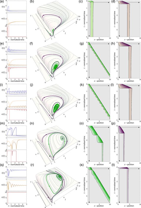
ONE-DIMENSIONAL CELL MOTILITY PATTERNS                                                  PHYSICAL REVIEW RESEARCH 2, 033237 (2020)

    FIG. 3. Stability analysis along the line k = 0.8 [vertical black
dashed line in Fig. 2(a)]. (a) The maximal and minimal length as
a function of r. (b) The maximal and minimal force applied on a
linker at the back part of the cell as a function of r. (c) The maximal
and minimal adhesion concentration at the rear as a function of r.
(d) The time period of the limit cycle as a function of r. Solid black
curves indicate the stable limit cycle. Dashed black curves indicate
the unstable limit cycle. Parameters: v = 10, κ = 20, and fs = 5.

cycle) to smooth motion (stable fixed point), as demonstrated
in Fig. 4.
   For increasing r, the separatrix grows until it meets the
limit cycle, which marks the transition to flows that all lead
to the single stable fixed point. The dynamics in this regime
correspond to a smooth motion of a slow moving and elon-
gated cell [Figs. 2(b)–2(d) and 3].                                           FIG. 4. [(a)–(c)] Dynamics in the bistability regime [red star in
                                                                          Fig. 2(a). (a) Blue and orange curves are the time series of the cell
                   3. Comparison to experiments                           length and adhesion concentration at the rear. Black dashed line
                                                                          indicates the time when noise was injected into the solution of the
    We now compare in detail the model’s stick-slip limit-cycle           differential equation [Eq. (17)]. (b) n-l phase diagram. Red curve
dynamics [Figs. 2(e)–2(g)] to experiments (see Appendix C                 is the trajectory and black curve is the separatrix between the two
for experimental methods). In Fig. 5, we analyze the stick-slip           modes of motion. (c) The corresponding kymograph: black curves
migration mode of a C6 glioma cell (seeded on laminin-coated              represent the edges of the cell xb and x f . Dashed black line indicates
lines of 5 μm width), by following the cell length and the                the time when noise was injected. Parameters: v = 10, k = 0.8, κ =
intensity of membrane-bound vinculin, using total internal                20, and fs = 5.
reflection fluorescence (TIRF) microscopy. As a component
of the adhesion complex, we denote the total intensity of
vinculin in the rear of the nucleus as a measure of the adhesion          change in some other internal parameter of the cell. Neverthe-
strength at the cell back in the model (n). We find that the              less, recent experiments [32] indicate that these glioma cells
experimentally observed dynamics during a stick-slip cycle                are highly sensitive to the adhesion strength, which strongly
give rise to a limit cycle in the n, l-phase space that has the           affects their migration behavior, as our model suggests. A
same qualitative features as the model predicts [Fig. 2(f)].              previous work [15] showed that dynamic changes in the
    The robust features of the migration modes predicted                  cell-substrate adhesion, as exposed by vinculin fluorescence
by the model can be observed in experiments (Fig. 6). In                  levels, can transform a cell from being stalled (i.e., extending
Fig. 6(a), we show a kymograph of a motile cell moving along              in both directions but remaining unpolarized) to motile. This
a one-dimensional stripe, exhibiting stick-slip behavior. At a            demonstrates that cells are poised close enough to the tran-
certain point along the trajectory, the cell increased both its           sition between these different modes, and naturally occurring
rate of stick-slip events, and its overall migration velocity. In         fluctuations in the adhesion strength are enough to move them
addition, the amplitude of the stick-slip events decreased in             across the transition line.
size. All of these features are captured by the model, if the                 Cell migration has been shown to be dramatically af-
average adhesion strength between the cell and the substrate              fected by changes in substrate composition [9]. In Fig. 24
(r) decreases abruptly along the trajectory, and the cell moves           (Appendix D), we provide a direct measure of the hetero-
from high to low r within the stick-slip regime [Fig. 2(a)].              geneities in the surface coverage by laminin along the one-
    In Fig. 6(b), we show a cell migrating smoothly, and then             dimensional stripes, which occur during the preparation of
abruptly decreasing in length and increasing in speed. This               these stripes. In particular, there are high concentration puncta
behavior is captured by the model assuming that the adhesion              deposited along the track, and moving across them could
strength r decreases such that the cell jumps from high to low            initiate abrupt changes in the cell-substrate adhesion strength.
r as shown in Figs. 2(a), 2(d) and 2(j).                                      Note that the backwards growth of the lamellipodia at
    Note that we can not exclude that the abrupt change in                the cell back [Fig. 6(a)], during each stick-slip cycle, are
behavior observed for the cells in Fig. 6 originates from a               described by the more elaborate model below. In addition,

                                                                    033237-5
RON, MONZO, GAUTHIER, VOITURIEZ, AND GOV                                                  PHYSICAL REVIEW RESEARCH 2, 033237 (2020)

    FIG. 5. Comparison of the basic stick-slip model [Eqs. (17)and (18)] to the stick-slip dynamics observed in experiments (patient-derived
Human glioma propagating cell NNI21 transfected with fluorescently tagged vinculin and seeded on laminin-coated lines of 5 μm width and
imaged every 110 sec). (a) Movie snap shots, where the cells have fluorescently labeled vinculin (represents the extent of adhesion complexes).
The region that defines the cell back is to the left of the vertical dashed line, i.e., behind the nucleus. (b) A kymograph of the cell migration,
with the stick slip events marked. (c) The dynamics of the cell length and the total amount of vinculin signal at the cell back region, as function
of time. The black line on both graphs indicates the stick-slip cycle used to plot the phase-space limit cycle shown in (d).

we observe highly dynamic stick-slip behavior at the leading                polarization of the cell. We use a modified version of the
edge of the cell, which are also associated with propagating                scheme developed in Ref. [26] [Fig. 7(a)], whereby in addition
actin waves [15], and which we do not describe by our current               to the advection of a “polarity-cue” protein that enhances
model [23,33].                                                              the actin treadmilling, such as myosin-II, we also consider a
                                                                            polarity-cue that acts as an inhibitor of actin polymerization.
                                                                            The inhibitor protein is free to diffuse in the cytoplasm, and is
           B. Polarized cell with a dynamic protrusion
                                                                            also advected by the actin treadmilling flow. An example for
                        1. Model description                                an inhibitor of local actin polymerization, that is advected by
   We now complement the length-adhesion model described                    the actin flow, is Arpin [26,34]. We furthermore assume that
above, by incorporating a model for the spontaneous self-                   the timescale of the redistribution of the polarity-cue protein

   FIG. 6. Comparison of the basic stick-slip model [Eqs. (17) and (18)] to experiments on C6 glioma cells seeded on laminin-coated lines of
5 μm width (imaged every 30 sec). Kymographs correspond to total time 2.5 hours. (a) Comparison to model results with r = 7, then abruptly
changed to r = 3 (indicated by the horizontal dashed line). (b) As in (a), with r = 8.5 then changing abruptly to r = 1. Model parameters:
v = 10, k = 0.8, κ = 20, and fs = 5.

                                                                    033237-6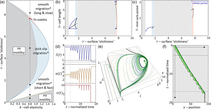
ONE-DIMENSIONAL CELL MOTILITY PATTERNS                                                    PHYSICAL REVIEW RESEARCH 2, 033237 (2020)

                                                                            our approximation of quasistatic boundary when calculating
                                                                            the polarity cue distribution is not valid. Nevertheless, these
                                                                            periods extend over a very small fraction of the cell migration,
                                                                            and we do not expect them to be significantly affect the overall
                                                                            validity of our results.
                                                                               We can therefore use the steady-state distribution of the
                                                                            concentration of this inhibitor c(x), which is given by an
                                                                            exponential function [Fig. 7(b)]

                                                                                                              e− D
                                                                                                                 vx
                                                                                                    ctot v
                                                                                             c(x) =                 vx  ,                     (19)
                                                                                                     D e− vxDb − e− Df

                                                                            where v is the effective instantaneous actin treadmilling ve-
                                                                            locity, D the effective diffusion coefficient of the inhibitor, and
                                                                            ctot is the total amount of inhibitor molecules in the cytoplasm
                                                                            (see Appendix E).
    FIG. 7. The stick-slip UCSP model. (a) Illustration of a the phys-          To complete the model [26], we need to relate the tread-
ical model. Unlike the simple model of Fig. 1, the treadmilling veloc-      milling flow of actin across the cell to the polarity cue gradi-
ity is now dependent on the cell length v(l ), due to the advection of an   ent. In Refs. [26,27], the treadmilling flow was assumed to
inhibitory cue. The concentration of the inhibitory cue is represented      be dominated by the imbalance in the contractile forces of
by the colorbar on the right. The steady-state concentration of the         myosin-II across the cell length, and myosin-II was treated
inhibitory cue, c(x), is shown in [(b), top], which is an exponential       as the polarity cue. Here we rather focus on the actin flow
function due to a balance between diffusion and advection [Eq. (19)].       due to polymerization activity at the two opposing ends of
The effect of c(x) on the local actin polymerization rate is given          the cell. We therefore treat c(x) as an inhibitor of actin poly-
by a Hill function [Eq. (20)] [(b), bottom]: where the inhibitory           merization, but similarly one could augment this by including
cue concentration is low the local actin polymerization rate is large.      an additional polarity cue that affects the treadmilling flow
(c) The steady-state retrograde flow speed as a function of cell length     due to myosin-II contractility. We focus in this work only
[solution of Eq. (21)]. Red solid line represent the stable solution.       on the contribution of the polymerization activity. The net
Red dashed line represent the unstable solution. Black dashed line          treadmilling flow is therefore given by the difference between
notes the critical length lc of polarization.                               the actin polymerization flows created at the two ends of the
                                                                            cell, which are inhibited by the local concentration of the
                                                                            inhibitor at the front and rear
(inhibitor) across the cell is much shorter than the timescale
of changes in the actin treadmilling speed. This assumption,                                  v(x f , xb ) =β(c̃(x f ) − c̃(xb )),            (20)
of separation of timescales, was also made in Ref. [26],
and is corroborated by recent measurements of myosin-II                     where β gives the scale of the actin flow in the cell, and
redistribution time when advected by actin (∼10 sec) [30],                  the polymerization activity at each end is diminished by the
while the stick-slip cycles of the cell are over timescales of              inhibitor concentration at each end, given by a Hill function
tens of minutes [9].                                                        [26,27]: c̃(xb, f ) = cs /(cs + c(xb, f )) [Fig. 7(b)], where cs is the
   Another key assumption which we make is of quasistatic                   concentration at which the effect of the inhibitor saturates.
boundaries when calculating the profile of the polarization                    After rescaling (see Appendix F), using Eqs. (19) and (20),
cue across the length of the cell, c(x) [in Eq. (19) below and              we obtain the following implicit equation for the net actin
derived in Appendix E]. Here, we work under the assumption                  treadmilling flow:
that the motion of the cell boundaries (i.e., its length changes)                             ⎛                                          ⎞
are slow compared to the redistribution of c(x) along the cell.                                          1                      1
Specifically, this amounts to the regime where the motion                         v(l ) = β ⎝                 −                1  ⎠. (21)
                                                                                                 1 + c Dv vl1          1 + c Dv     − vl
of the cell boundaries is slow compared to the actin flow,                                               e D −1                 1−e   D

such that the rate of cell-length change obeys l˙  v [see
Eqs. (E6) and (E7)]. Within this regime, we can solve the                       In the persistent regime (sufficiently large cs ), we find that
steady-state c(x) considering the boundaries to be static and               as l increases above a critical value Eq. (21) undergoes a pitch-
solving at each time according to the instantaneous length and              fork bifurcation, where spontaneous actin treadmilling ap-
the treadmilling actin flow v. The timescale of the stick-slip              pears, corresponding to a polarized and motile cell [Fig. 7(c)].
cycle is of tens of minutes, and this is longer than the timescale          The critical length is given by
over which we expect the polarity cue to redistribute within                                                       c
the cell. For example, a polarity cue that enhances local actin                                       lc =                 ,                 (22)
treadmilling, myosin-II, was recently observed to redistribute
                                                                                                                  cβ
                                                                                                                  D
                                                                                                                       −1
on a much shorter timescale of tens of seconds [30], and there-
fore supports the validity of our approximation. However,                   which provides a lower bound for the coupling strength β >
during a slip event, the cell does change its length rapidly, on            D/c, below which there is no spontaneous motility. A lower
the order of tens of seconds. During these very short periods,              critical length for polarization was also obtained in Ref. [35].

                                                                      033237-7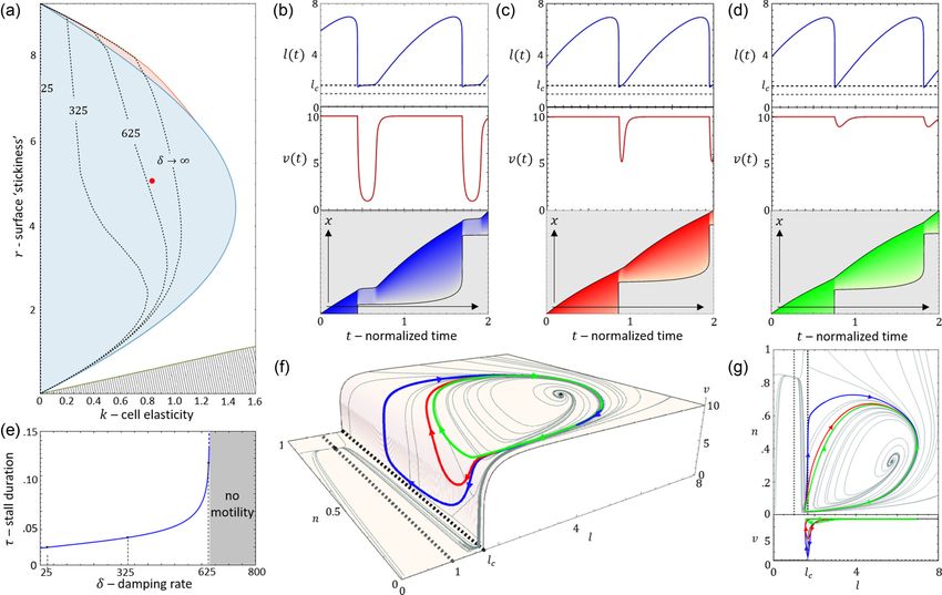
RON, MONZO, GAUTHIER, VOITURIEZ, AND GOV                                                    PHYSICAL REVIEW RESEARCH 2, 033237 (2020)

   FIG. 8. (a) k-r phase diagram. Striped texture regions correspond to regimes where there is no motility (stationary cell). Blue region
corresponds to a bistable region of polarized stick-slip cells and stationary cells. White region corresponds to bistability between stick slip and
smooth migration. Red region corresponds to tristability between stick slip, smooth migration, and stationary cells. Blue/red/brown curves
are the Hopf/saddle node/Hopf bifurcation transition lines. Black dashed line is the r cross section for k = 0.8. Black dots correspond to
the points (k, r) = (0.8, 0.4), (0.8, 0.7), (0.8, 1.65), (0.8, 5), (0.8, 8). Red star correspond to the point (k, r) = (0.8, 7.7). (b) Maximal and
minimal amplitude of the l state variable as a function of r for the limit cycles in the vector field along the cross section of k = 0.8. Dashed
blue curve correspond to the unstable discontinuous limit cycle. Solid black curve corresponds to the stable limit cycle and the cell length.
Black dashed curve is the unstable limit cycle. (c) The time period of the limit cycles. Blue dashed line indicate the discontinuous unstable limit
cycle. Black solid line indicate the stable limit cycle (period of stick slip). Black dashed line indicates the unstable limit cycle in the tri-stable
region. [(d)–(f)] The tristable region. Solution of Eqs. (23) and (24) with noise of amplitude (δl, δv) = (0.5, 0.11) injected at t = 3.55 and
(δl, δn) = (0.5, 0.05) injected at t = 16.2, to demonstrate the transition between the phases (across the separatrix lines). Blue/orange/red
curves in (d) correspond to the dynamics of length/adhesion concentration and actin retrograde flow. Gray dashed lines indicate the time point
in which the noise was injected. Green curve in (e) is the trajectory in the l-n-v phase space. Black solid lines are the separatrices. (f) displays
the kymograph which corresponds to [(d) and (e)]. Parameters: fs = 5, κ = 20, β = 11, c = 3.85, and D = 3.85.

   The equations of motion are now extended beyond the                       length for polarization. In this case, we find another fixed
basic model [Eqs. (17) and (18)] to include the dynamics of                  point that corresponds to v = 0
the actin treadmilling flow
                                                                                                  ∗ ∗           r
                                                                                               l , n = 1,                         (26)
                                     exp k(l−1)
                                             n f                                                                1+r
             l˙ =v − k(l − 1) 1 +                s
                                                       , (23)
                                           n                                 where the cell is at its rest length and stationary.

                                       k(l − 1)
                ṅ =r(1 − n) − n exp                 ,   (24)
                                          n fs                                                              2. Results
                       v̇ = − δ(v − vss (l )),                     (25)         In Fig. 8(a), we plot the k-r phase diagram for the simpler
                                                                             case of δ → ∞, such that the actin flow speed is given directly
where vss (l ) is the steady-state solution to Eq. (21), which               by the solution vss (l ) [Eq. (20), Fig. 7(c)]. In comparison with
is the length-dependent actin flow speed, and δ is the rate at               the case of fixed actin flow [Fig. 2(a)], there are several new
which the actin flow adjusts to length changes, i.e., the rate at            phases, despite the overall similar shape of the phase diagram.
which v approaches vss (l ).                                                    For very low values of r, we find that there is a transition
    For a cell that has a rest length that is longer than the critical       line below which the cell is nonmotile [brown region in
length for polarization, lc < 1, the resting state of the cell is            Fig. 8(a)], which corresponds to all the flows in the n-l phase
polarized. Since the velocity saturates to a constant value for              space leading to the single fixed point at v = 0 [Eq. (26)].
l > lc [Fig. 7(c)], the results are qualitatively similar to those           Above this transition line, with increasing r, there are phases
we obtained for a constant, length-independent, v (Fig. 3).                  of coexistence between smooth motion or stick slip, and non-
    We will therefore focus on the more interesting case where               motile behavior. We plot in Fig. 9 the dynamics for different
lc > 1, and the rest length of the cell is smaller than the critical         points of increasing value of r, for fixed k = 0.8 [vertical

                                                                     033237-8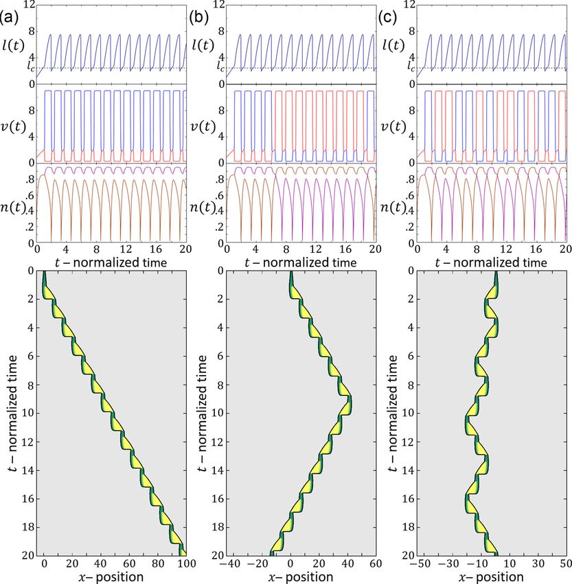
ONE-DIMENSIONAL CELL MOTILITY PATTERNS                                                    PHYSICAL REVIEW RESEARCH 2, 033237 (2020)

    FIG. 9. The dynamics along the line of constant k = 0.8 [vertical dashed line in Fig. 8(a)]. [(a)–(d)] r = 0.4, [(e)–(h)] 0.7, [(i)–(l)] 1.65,
[(m)–(p)] 5, and [(q)–(t)] r = 8. Blue/orange/red curves in (a), (e), (i), (m), and (q) correspond to the time series of the cell length, adhesion
concentration and actin retrograde flow respectively (bold/thin lines corresponds to green/purple trajectory). Green and purple lines (b), (f),
(j), (n), and (r) demonstrate the trajectories in the bistable l-n-v phase space regime. Black solid curves are the separatrices. (d), (g), and (i)
display the corresponding kymographs. Parameters: fs = 5, κ = 20, β = 11, c = 3.85, and D = 3.85.

                                                                    033237-9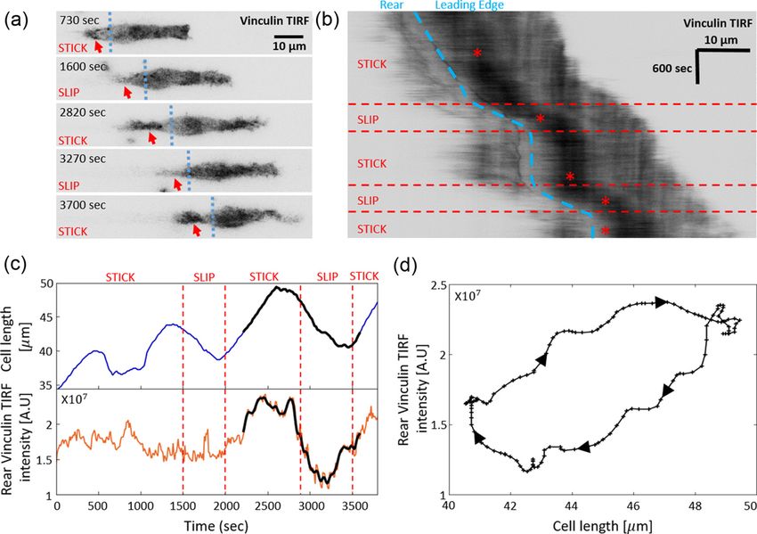
RON, MONZO, GAUTHIER, VOITURIEZ, AND GOV                                                    PHYSICAL REVIEW RESEARCH 2, 033237 (2020)

    FIG. 10. The effect of a finite actin response rate δ on the dynamics [Eq. (25)]. (a) The k-r phase diagram for different values of δ [in
Eq. (25)]. Dashed black lines indicate the coalescence of the discontinuous unstable and stable limit cycles, which produce the no-motility
regime for different values of δ. The phase transition line for δ → ∞ is the same as in Fig. 8(a). [(b)–(d)] Demonstration of the lagging time
for values of δ at the point (k, r) = (0.8, 5) on the phase diagram (black dot). Blue and red curves are the time series of the cell length and actin
retrograde flow speed, respectively. Black dashed line is the critical length of polarization and gray dashed line is the rest length of the cell.
Blue, red, and green kymographs correspond to δ = 625, 325, and 25 respectively. (e) The duration of the stall as a function of δ, indicating
the values of δ = 625, 325, and 25 at the point (k, r) = (0.8, 5). Gray region indicates where there is no motility for every initial condition.
(f) The stable limit cycles which correspond to (b)–(d) in the l-n-v phase space. (g) Projections of the stable limit cycles which correspond to
(b)–(d) in the l-n and l-v phase spaces. Other parameters: fs = 5, κ = 20, β = 11, c = 3.85, and D = 3.85.

dashed line in Fig. 8(a)]. Two flows are demonstrated for each               drop to zero instantaneously (as in the case when δ → ∞).
case (green and purple paths and corresponding kymographs                    There is therefore a region of the phase diagram where the
in Fig. 9), exposing the coexistence of either smooth motion                 length recovers and increases above lc , allowing the stick-slip
[(e)–(h) and (q)–(t)] or stick slip [(i)–(l)] with the nonmotile             limit cycle to survive. The “stall duration,” during which l <
phase. The bifurcations of the stable and unstable solutions are             lc and the cell is almost stalled, increases with increasing value
denoted by their cell length (and the limit cycle amplitude), as             of δ [Fig. 10(e)].
well as the limit cycle periods, in Figs. 8(b) and 8(c) (along
the same k = 0.8 line).                                                        C. Self-polarized symmetric cell with a dynamic protrusion
   There is even a thin region of tristability [Fig. 8(a)], which
we demonstrate in Figs. 8(d)–8(f), by inducing a transition                                          1. Model description
between the three phases by adding noise at specific times.                     In the model, we developed so far, we did not allow for the
For a complete exploration of the k-r phase diagram see                      actin polymerization to produce local traction and protrusive
Appendix G.                                                                  forces at both ends, but rather assumed that the competition
   Next, we explore the effect of a finite value of δ, where                 between the two ends gives rise to a single leading edge (or to
the treadmilling velocity of the actin does not instantaneously              an unpolarized cell) [Fig. 7(a)].
adjust to its length-dependent value vss (l ) [Eq. (25)].                       We now extend the model to describe the local protrusive
   In Fig. 10(a), we plot the shift in the stick-slip transition             forces that are produced by actin polymerization at the two
line to lower values of k, for decreasing values of δ. The region            ends of the cell [Fig. 11(a)].
of no-motility is now pushed to lower values of k. The reason                   The dynamics of the moving front and back depend on their
for this is shown in Figs. 10(b)–10(d): when the length drops                respective direction of motion: when they protrude there is a
below lc after the slip event, the velocity of the actin does not            drag force that is given by a constant drag coefficient, while

                                                                    033237-10
ONE-DIMENSIONAL CELL MOTILITY PATTERNS PHYSICAL REVIEW RESEARCH 2, 033237 (2020)
Similarly, the dynamics of the adhesions are given by
−v f /b + k(x f − xb − 1)
ṅ f /b = r(1 − n f /b ) − n f /b exp .
fs n f /b
(29)
The dynamics of the polymerization/tread-milling of the actin
is now calculated separately on both sides of the cell, given by
v̇ f /b = −δ(v f /b − v ∗f /b ), (30)
where
cs
v ∗f /b = β . (31)
cs + c̃(x f /b )
The distribution of the inhibitor along the cell is affected
by the competition between the treadmilling actin from both
ends, so its given by Eq. (19) with: v = v f − vb .
FIG. 11. The symmetric model. (a) Illustration of the physical
model. xb and x f are the back and front part of the cell which are 2. Results
connected by a spring with a stiffness k. x0 is the rest length of the
spring and l is the length of the cell. v f and vb are the steady-state The solution of Eq. (31) is shown in Fig. 11(c). The
velocities of actin retrograde flow from both ends of the cell, which solution shows that the cell remains unpolarized for l < lc ,
are coupled to the gradient of an inhibitory cue. The concentration and the actin tredmilling flows are equal at the two ends of the
of the inhibitory cue is represented by the colorbar on the left. At cell, given by v f /b = β(l/(c + l )). A polarized cell for l > lc
both ends of the cell, three forces act: a protrusion force (red arrow), has a higher treadmilling flow from the front, and in the limit
which is proportional to the retrograde flow speed (dark red arrow), of large l the treadmilling velocity approaches these limiting
a drag force (teal arrow) when the edge is moving forward, and values: v ∗f = β and vb∗ = D/c.
a friction force due to the slip bonds (blue arrow) when the edge We find that there is a new length scale in the system,
is moving backwards. (b) Demonstration of the friction model in which determines the ability of the cell to elongate and reach
Eq. (28): upper panel displays in blue the derivative of the moving polarization. For the unpolarized cell, we equate the protrusive
rear ẋb . Below in orange is the Heaviside theta function of the time forces at both ends to the restoring force of the spring
series of ẋb . Right panel displays the corresponding kymograph.
l
(c) The steady-state retrograde flow speed as a function of cell length k(l − 1) = β , (32)
[Eq. (31)]. Red solid line represents the stable solution. Red dashed c+l
line represents the unstable solution. Black dashed line denotes the
which yields the polarization length
critical length of polarization lc . Parameters: β = 19, c = 9, and
D = 40.
1 β 1 β 2
l p = (1 − c) + + c+ (c − 1) − . (33)
2 2k 2 2k
when they retract the friction depend on the slip-bond activity
By equating the critical length lc (22) to the polarization length
of the adhesion [Fig. 11(b)]. We therefore have the following
l p (33), we obtain a critical value of β, above which the cell
equations of motion for the two ends of the cell:
polarizes [Figs. 12(a) and 12(b)]
1
ẋ f /b = (±v f /b ∓ k(x f − xb − 1)), (27) d c2 k 2
f /b βc = + ck +
2c 2d
where the friction coefficients are given by ck − d 2
+ d + 2c(1 + 2c)dk + c2 k 2 . (34)
2cd
f /b = 1 − (∓ẋ f /b )
As for the previous model (Sec. II B), the interesting behav-
v f /b − k(x f − xb − 1) ior is for a cell that has a rest length that is smaller than lc > 1.
+ (∓ẋ f /b )n f /b κ exp ,
fs n f /b For such a system we demonstrate the dynamics for different
(28) values of β (above and below βc ), in Figs. 12(d)–12(l). For
β < βc , the cell elongates symmetrically [Figs. 12(d)–12(f)],
where is the theta Heaviside function. This way the friction but does not polarize (no spontaneous symmetry breaking).
coefficient depends on the local motion of each end. This is For β > βc , we find regimes of smooth motion [β = 8,
illustrated in Fig. 11(b), where the friction at the back is due Figs. 12(g)–12(i)] and stick slip [β = 11, Figs. 12(j)–12(l)]
to the slip-bonds when the back end of the cell is retracting for parameters that correspond to these phases in the phase
ẋb > 0 and (ẋb ) = 1. diagram of the stationary treadmilling system (Fig. 2). Note
Note that the force that pulls on the adhesions during that for any fixed value of β Eq. (34) provides a critical value
retraction [in the exponential function in Eq. (28)] is not only of the cell stiffness k, above which β < βc and the cell can not
given by the elastic spring force (as in the previous models elongate over the critical length, so becomes immobile.
presented above) but is countered by the local force of actin When the cell is within the stick-slip regime, it may end
polymerization that is pushing the membrane. up after each slip event with a cell length that is shorter than
033237-11RON, MONZO, GAUTHIER, VOITURIEZ, AND GOV PHYSICAL REVIEW RESEARCH 2, 033237 (2020)
FIG. 12. The polarization length. (a) The critical length lc (blue) and polarization length l p (orange) as a function of the coupling coefficient
β. Gray dashed lines indicate the sample points of β = 4, 8, and 11. (b) The steady-state velocity profile as a function of length for β =
4, 8, and 11 (purple, teal, and yellow curves, respectively). (c) The critical coupling coefficient as a function of cell elasticity k. The purple,
teal, and yellow dashed curves denote the critical values of k for the values of β used in (b) and (d)–(l). The black dashed line denotes
the critical value of β for k = 0.8 [which is the value of k used in (d)–(l)]. [(d)–(f)] Time series, kymograph, and phase space for β = 4.
[(g)–(i)] Time series, kymograph, and phase space for β = 8. [(j)–(l)] Time series, kymograph, and phase space for β = 11. In (d), (g), and
(i), the upper blue curve is the time series of the cell length. Dashed black/gray lines are the critical/polarization lengths. Lower red/blue
curves represent the time series of the actin retrograde flow speed at the front/back respectively. In (e), (h), (k), the purple/teal/yellow colors
represent β = 4, 8, and 11. In (f), (i), and (l), the red/blue curves represent the trajectories at the l-n f -v f /l-nb -vb phase spaces (upper/lower
part of the surface). Parameters: κ = 20, fs = 5, r = 5, k = 0.8, c = 3.85, δ = 250, and D = 3.85.
033237-12ONE-DIMENSIONAL CELL MOTILITY PATTERNS PHYSICAL REVIEW RESEARCH 2, 033237 (2020)
FIG. 13. Time series of the cell length (dark top panels) and the retrograde flow speed (bottom) of the symmetric system for different
values of the parameter c: (a) c = 3.85, (b) 7.7, and (c) 11.55. Black dashed line in the upper panels is the critical length of polarization
lc . Red/blue curves in the lower panels represent the actin flow at the front/back. Other parameters: β = 11, D = 3.85, f s = 5, κ = 20, r =
5, k = 0.8, and δ = 250.
lc . Since in the symmetric model the protrusive force acts overall migration velocity. This is demonstrated in Figs. 14
locally at both ends, the cell elongates symmetrically until and 15.
l > lc and it repolarizes. This is demonstrated in Fig. 11(b). During each stick-slip event, since the cell loses polarity, it
In Fig. 13, we show the effect of the parameter c on the may repolarize in a new direction. This occurs when we add
stick-slip migration, where increasing c increases lc [Eq. (22)] random noise to the equations of motion: the system is solved
and increases the time it takes the cell to repolarize following as a stochastic differential equation where additive noise is
each slip event. added to the actin flow v f and vb . For different amplitudes
Furthermore, since the cell is effectively stalled when its of the noise term, we plot in Fig. 16(a) the probability p that
length is shorter than lc , the time it takes for the cell to the cell changes its direction of motion per stick-slip event.
expand back to lc after each stick-slip event determines the We find that for each level of noise there is a critical value
FIG. 14. The effect of lc on the overall velocity of migration during stick slip: [(a)–(c)] Above the critical length. c = 3.95, r =
3, 5, and 7. (Left) kymograph, (right top) cell length and speed time series. (Bottom) phase space. Parameters: β = 11, D = 3.95, k =
0.8, fs = 5, κ = 20, δ = 210. [(d)–(e)] Below the critical length. c = 11.85, r = 3, 5, and 7. (Left) kymograph, (right top) cell length and
speed time series. (Bottom) Phase space. Parameters: β = 11, D = 3.95, k = 0.8, fs = 5, κ = 20, and δ = 210.
033237-13RON, MONZO, GAUTHIER, VOITURIEZ, AND GOV PHYSICAL REVIEW RESEARCH 2, 033237 (2020)
FIG. 15. Effect of lc on the overall migration velocity during stick-clip motion. [(a)–(c)] Cell length is above the critical length. c = 5, r =
2, 4, and 6. (Left) Kymograph, (right top) cell length and speed time series. (Bottom) phase space. Parameters: β = 11, D = 3.95, k =
0.8, fs = 5, κ = 20, and δ = 210. [(d)–(e)] Below the critical length. c = 6, r = 2, 4, and 6. (Left) Kymograph, (right top) cell length and
speed time series. (Bottom) phase space. Parameters: β = 14, D = 20, k = 1, fs = 5, κ = 20, and δ = 120.
of the actin response rate δ [Eq. (30)] that sets a threshold rise to other stick-slip regimes observed in the experiment:
between p = 0 and 0.5. During each stick-slip event, when a cell with low-frequency of small-amplitude stick-sip events
l < lc , the actin flow velocities on both sides approach each (Fig. 20), and a cell with high-frequency of large-amplitude
other exponentially with a timescale of δ −1 . As v f /b approach stick-slip events (Fig. 21).
within the noise amplitude, they cross each other [Figs. 16(b) In Fig. 22, we give a wide range of different cell migra-
and 16(c)], and the side that has the higher flow when l = lc tions observed in experiments, demonstrating that the model
determines the new direction of cell motion. The dynamics can produce a similar range of cell migration patterns. In
around the critical δ where the turning probability increases Fig. 22(a), we show a cell that seems to be oscillating between
strongly, are demonstrated in Fig. 17. being polarized to the right and to the left, such that it hardly
migrates over time. In our model, a similar behavior may
occur if the cell is in the stick-slip regime, and following each
III. COMPARISON TO EXPERIMENTS
slip event it is shorter than the critical length, allowing for
When comparing the results of our fully symmetric model noise to induce direction changes (as explained in Figs. 16
to the experimental observations of motile cells along one- and 17).
dimensional tracks, we need to note that the cellular system is In Fig. 22(b), a kymograph is shown of a cell that is initially
very noisy. Nevertheless, our model exposes distinct motility at rest, and elongates symmetrically. At some later time it
patterns that should underlie the noisy motion of the cells. breaks the right-left symmetry and moves in a persistent
First, we wish to show that the main classes of cell be- manner. This behavior is well described by our model, where
haviors, which is observed within a uniform population of the rest-length of the cell is below the polarization length,
identical cells (Fig. 18) can be qualitatively spanned by the but the conditions are such that β > βc and it elongates
model if, for example, the actin treadmilling activity (model symmetrically until it reaches a length that is longer than the
parameter β) is variable within the population. critical length lc . At a later time point we decreased the value
Next, we focus on the stick-slip migration pattern, and of the surface adhesion strength r, leading to a transition from
compare several examples of such observed cell trajectories long-slow to short-fast migration mode, which seems to fit this
to the dynamics predicted by the model (Fig. 19). We find that cellular behavior (similar to Fig. 6).
there is strong similarity between the dynamics exhibited by In Fig. 22(c), we plot a kymograph of a cell that is persis-
the cell and in the model, regarding the oscillations in the cell tently moving on a 1D track in the stick-slip regime. During
length and velocity. The limit-cycle trajectory predicted by the each stick-slip event the progression of the cell’s leading edge
model can be observed in the experimental data. For slightly is slightly modulated, while at the back there are periodic
different set of parameters, we find that the model gives extensions of lamellipodia that undergo large retractions. This
033237-14ONE-DIMENSIONAL CELL MOTILITY PATTERNS PHYSICAL REVIEW RESEARCH 2, 033237 (2020)
mode, or correspond to regimes where different migration
modes coexist. The transitions in the cell behavior from one
migration mode to another may therefore correspond to the
dynamics of the internal parameters of the cell. In addition,
noise in the dynamical variables (such as in the actin tread-
milling speed), can drive the enhanced polarization changes
observed during stick-slip motion.
IV. CONCLUSION
Cell motility involves a large number of cellular com-
ponents, connected by a complex network of interactions.
In addition, the system is noisy, which makes the analysis
of cell migration a daunting task. In the present work, we
developed a theoretical model aimed at exposing the motility
patterns of cells moving along a one-dimensional track. One
dimensional motion is both simpler to analyze experimentally,
and describe theoretically, as well as being highly relevant
to cells migrating within tissues during development [17,18]
and cancer progression [16,19]. It is also considered to be
closely related to the migration of cells in many types of
three-dimensional environments [36,37].
We find that the coupling between the cell length and
the slip-bonds of adhesion molecules, through the spring-
like elasticity of the cell, provides the basic mechanism of
stick-slip during cell migration. Furthermore, we show that
when cells migrate and their polarization is maintained by the
overall actin treadmilling flow, the cell length couples strongly
to the polarization state of the cell: cells below a critical
length do not polarize. While persistent smooth and stick-slip
migration modes arise naturally in our model, we predict
that stick-slip events may allow for noise-induced direction
changes, as the cell recoils to less than the critical length at
each stick-slip cycle.
The minimal model that we present recovers the rich
FIG. 16. (a) The probability to change direction as a function of
variety of cellular migration patterns, which we then compare
the damping rate for different levels of noise in the actin velocity.
to experiments on migrating cancer cells (glioma). These
(b) Demonstration of a stick slip event at which the noise level is
low (v = 10−3 ), such that v f (blue) and vb (red) do not cross when
comparisons validate the model and demonstrate how it can
l < lc , and the cell remains polarized. (c) Demonstration of a stick provide the framework for understanding the complex migra-
slip event at which the noise amplitude is sufficiently high (v = tion patterns exhibited by migrating cells.
10−2 ), such that v f (blue) and vb (red) cross when l < lc , which Our model makes detailed predictions regarding the depen-
enable the polarization mechanism to switch directions. Parame- dence of the cellular migration modes on the coarse-grained
ters: κ = 20, fs = 5, r = 5, k = 0.8, c = 11.55, D = 3.85, β = parameters of the model, which describe the cell’s mechanics
11, and δ = 300. (k), actin-polymerization activity (β) and surface adhesion (r).
We predict a reentrant smooth migration regime as function
of the surface adhesion, with stick-slip occurring only at the
behavior corresponds very well to the stick-slip behavior in intermediate regime (Figs. 2, 8, and 10).
our model. Despite the fact that the motile behavior of cells is highly
Finally, in Fig. 22(d), we present a kymograph of a cell that dominated by noise, our model helps to expose the underlying
is first observed to be migrating by slow stick-slip events. At deterministic patterns of motility [27] that drive the cellular
some point the cell stops and rounds up, as it enters mitosis, motion, which may be partially masked by noise. We show
from which two daughter cells emerge, both migrating with that the noise can also drive dramatic transitions between the
similar speeds, but one seems to be moving smoothly while different motility patterns, since the cell may reside close to
the other exhibits some stick-slip cycles. We demonstrate the transition lines, or in a regime of coexistence, between
a similar chain of migration changes using our model, by such modes. These results offer a new explanation for the
modulating the parameters that determine the actin tread- large “phenotypic heterogeneity” (CCV) that is observed in
milling activity (β) and adhesion strength (r). cell migration experiments, even under well controlled con-
These comparisons serve to show that the model can de- ditions and monoclonal cell population. These results offer
scribe the complex migration patterns of cells. The parameters a new framework to explain experimental observations of
used in the model may correspond to a unique migration migrating cells, resulting from noisy switching between un-
033237-15You can also read