Space Shuttle Debris Impact Tool Assessment Using the Modern Design of Experiments
←
→
Page content transcription
If your browser does not render page correctly, please read the page content below
Space Shuttle Debris Impact Tool Assessment
               Using the Modern Design of Experiments

                                            Richard DeLoach*
                        NASA Langley Research Center, Hampton, Virginia 23681-2199

                                             Elonsio M. Rayos†
                                  NASA Johnson Space Center, Houston, Texas

                                           Charles H. Campbell‡
                                  NASA Johnson Space Center, Houston, Texas

                                            Steven L. Rickman§
                                  NASA Johnson Space Center, Houston, Texas

                                                       and

                                             Curtis E. Larsen**
                                  NASA Johnson Space Center, Houston, Texas

           Complex computer codes are used to estimate thermal and structural reentry loads on
        the Shuttle Orbiter induced by ice and foam debris impact during ascent. Such debris can
        create cavities in the Shuttle Thermal Protection System. The sizes and shapes of these
        cavities are approximated to accommodate a code limitation that requires simple “shoebox”
        geometries to describe the cavities—rectangular areas and planar walls that are at constant
        angles with respect to vertical. These approximations induce uncertainty in the code results.
        The Modern Design of Experiments (MDOE) has recently been applied to develop a series of
        resource-minimal computational experiments designed to generate low-order polynomial
        graduating functions to approximate the more complex underlying codes. These polynomial
        functions were then used to propagate cavity geometry errors to estimate the uncertainty
        they induce in the reentry load calculations performed by the underlying code. This paper
        describes a methodological study focused on evaluating the application of MDOE to future
        operational codes in a rapid and low-cost way to assess the effects of cavity geometry
        uncertainty.

                                                Nomenclature
ANOVA           =   ANalysis Of Variance
BLT             =   Boundary Layer Transition
BPZ             =   Body Point Zone, a sub-area on the windward side of the Orbiter
CPU             =   Central Processing Unit
CV              =   Coefficient of Variation. Ratio of standard error to mean response
ET              =   External Tank
FS              =   Factor of Safety

*
   Senior Research Scientist, Aeronautical Systems Engineering Branch, NASA Langley Research Center, MS 238,
4 Langley Blvd, Hampton, Virginia 23681, Senior Member.
†
  Aerospace Engineer, NASA Johnson Space Center, Houston, Texas.
‡
  Aerospace Engineer, NASA Johnson Space Center, Houston, Texas, Senior Member.
§
  Chief, Thermal Design Branch, NASA Johnson Space Center, Houston, Texas.
**
   NESC Discipline Expert for Mechanical Analysis, NASA Johnson Space Center, Houston, Texas, Member.

                                                       1
                               American Institute of Aeronautics and Astronautics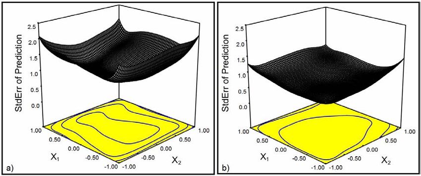
Inference space   =   A coordinate system in which each axis corresponds to an independent variable
ITA               =   Independent Technical Authority
JSC               =   Johnson Space Center
LaRC              =   Langley Research Center
LOF               =   Lack of Fit
MDOE              =   Modern Design of Experiments
MMT               =   Mission Management Team
MS                =   Margin of Safety
NESC              =   NASA Engineering and Safety Center
OBSS              =   Orbiter Boom Sensor System
OFAT              =   One Factor At a Time
OOPD              =   Out Of Plane Deflection
RCC               =   Reinforced Carbon-Carbon
RSM               =   Response Surface Modeling/Methods
RTF               =   Return to Flight
RTV               =   Room Temperature Vulcanized
SIP               =   Strain Isolation Pad
Site              =   A point in an inference space representing a unique combination of independent variables
TAEM              =   Terminal Area Energy Management
TMM               =   Thermal Math Model
TPS               =   Thermal Protection System
USA               =   United Space Alliance

                                                I.   Introduction

A     S part of the Space Shuttle Return-to-Flight (RTF) efforts, the ability to perform assessment of damage to the
      Shuttle Thermal Protection System (TPS), tiles and reinforced carbon-carbon (RCC), became vital to clearing
the vehicle for flight readiness and atmospheric entry. In order to accomplish this, a considerable amount of testing
and analysis was performed to determine whether a given TPS damage was considered to be survivable. A
combination of new and existing math model tools was developed to determine the impact tolerance and damage
tolerance of the TPS due to impacts from debris, primarily ice and foam from the external tank (ET). These math
model tools include damage prediction, aeroheating analysis, thermal analysis and stress analysis. Some tools are
physics-based and others are empirically based. Each tool was created for a specific use and timeframe, such as,
probability risk assessment, and real-time on-orbit assessment. In addition, the tools are used together in an
integrated strategy for assessing impact damage to tile and RCC.
    A peer-review of the tools to assess the engineering readiness for supporting RTF was initiated. The objective of
the peer review was to determine if the tools and the end-to-end strategy were suitable to support RTF. As part of
the effort to fully understand the limitations and sensitivities of the analytical tools, a task jointly funded by the
NASA Engineering and Safety Center (NESC) and the Independent Technical Authority (ITA) was initiated as a
collaboration of the NASA Johnson Space Center, the NASA Langley Research Center, and Jacobs Technology
team members. The scope of this assessment was limited to tile damage.
    Utilizing these tools requires knowledge of a variety of input parameters. As with any analysis, an understanding
of the sensitivity of the model response to the variation of the input parameters is essential. Additionally, since the
end-to-end analysis involves a variety of analysis steps utilizing multiple models and crossing disciplines, an
assessment of end-to-end uncertainty in the analysis was deemed necessary.
    The suitability of a Modern Design of Experiments (MDOE) approach was investigated for assessing the
analytical models’ sensitivity and end-to-end uncertainty. These analyses involve a large number of input variables.
To fully investigate all possible combinations of the parameters deterministically or by Monte Carlo sampling was
deemed infeasible. The MDOE approach showed promise in making the assessments more efficiently.

                                      II.   Analytical Model Overview
    Three-dimensional TPS damage thermal math models were developed to aid in the assessment of damage
sustained by the Orbiter tile during ascent. On-orbit inspection of the vehicle TPS by the Orbiter Boom Sensor
System (OBSS) provides a point cloud geometry of the damage that is subsequently used to develop simplified
representations of tile damage for use in the thermal model.

                                                         2
                                 American Institute of Aeronautics and Astronautics
The thermal response of the damaged region during atmospheric entry is assessed to predict tile and structural
temperatures in and around the damaged area. These temperatures are then superimposed with the entry mechanical
loads on a structural model to determine the structural integrity of the tile and vehicle structure. The results of this
analysis will be used to aid the determination by the Mission Management Team (MMT) of whether an observed
damage is acceptable to “fly as is,” or a repair will be attempted before reentry, or that safe reentry is not an option
in the damaged state and the Space Shuttle crew must remain on the International Space Station until a rescue
mission can be launched. Because of the dire consequences of an ill-informed decision, understanding the
uncertainty in this analysis is vital to the MMT.
    Three analytical tools make up the core of the damage assessment modeling capability developed by the United
Space Alliance and the Boeing Company team for the NASA Orbiter Project Office:
    1) The 3-D Thermal Math Model (3-D TMM) tool predicts the temperature response of the Orbiter lower
          surface acreage TPS materials and structure at damaged tile locations, using simplified tile damage
          geometries, structure definition, tile thickness, and material thermal properties. The tool predicts time
          histories of tile and structure temperatures, and structural thermal gradients.
    2) The RTV Bondline Tool calculates stresses for the Orbiter lower surface 6 in. × 6 in. acreage tiles at the tile-
          to-strain isolation pad (SIP) interface using tile damage dimensions, tile bondline temperature data from the
          3-D TMM tool and out-of plane deflections (OOPD) from the stress assessor tool. The tool defines factors
          of safety at the tile/strain isolator pad (SIP) interface of the damaged tile for tension in the RTV bond or
          tile, compression and shear of the tile, and shear in the SIP.
    3) The Stress Assessor Tool converts damage site local temperature increases into thermal loads. The tool
          combines these increased thermal loads with existing mechanical loads and analyzes the new set of
          combined loads using existing documented flight certification analysis programs to define Orbiter
          structural margins of safety and Orbiter surface out-of-plane deflections in the area near a tile damage site
          or tile repair site.
    The tool parameter inputs describing the idealized tile damage cavity (an inverted rectangular pyramid
geometry) are the length, width, and depth of the damage as measured at the top of the tile surface, and the angles of
the entrance, side, and exit faces. Length, width, depth, entrance angle, and side angle were the five independent
cavity geometry variables selected to define the polynomial response models for this study, with the decision to hold
exit angle fixed at 75°. This decision was predicated on preliminary results that revealed relatively little impact of
exit angle changes on computed reentry loads, at least over the range of 70° to 80°, which prior experience suggests
is typical for exit angles.
    In addition to the five independent geometry variables, two Shuttle state variables were identified. The first,
boundary layer transition time, serves as a surrogate for surface roughness and was defined as a categorical variable
with two fixed levels, 900 seconds and 1200 seconds, selected to bracket the anticipated range of this variable. The
second, baseline heating, was likewise established as a two-level categorical variable, representing low and
moderate baseline heating conditions.
    Tool output parameters of interest are tile bondline temperature, structural temperature, tile factor of safety, and
structural margin of safety. In addition, tile out of plane deflections for two regimes of the reentry trajectory were
also examined. The first regime was from Mach 25 to Mach 4, and the second regime was the Terminal Area Energy
Management (TAEM) regime, from Mach 4 to touchdown.

                           III.    Overview of Modern Design of Experiments
    The Modern Design of Experiments (MDOE) is a formal method of empirical investigation first introduced at
Langley Research Center in 1997 to enhance quality and productivity in large-scale, high-cost experiments, initially
wind tunnel experiments.1 It consists of integrated design, exaction, and analysis elements intended to extend
conventional industrial design of experiments technology (generally used for process and product improvement) to
cover the special circumstances of aerospace research. Such circumstances include a very low tolerance for
unexplained variance in experimental data, coupled with generally complex relationships between system response
variables of interest and the independent variables upon which they depend. The MDOE method is a general
approach to experimentation, and while initially motivated by productivity and quality issues in wind tunnel testing,
MDOE applications have rapidly expanded to include a wide range of aerospace disciplines, including
computational experiments.
    The mechanism by which MDOE improves both quality and productivity is to alter the focus of experimentation
from a traditional emphasis on data acquisition to an explicit concentration on the extension of knowledge. While
data acquisition rate and resulting data volume have been traditional measures of productivity in large-scale

                                                          3
                                  American Institute of Aeronautics and Astronautics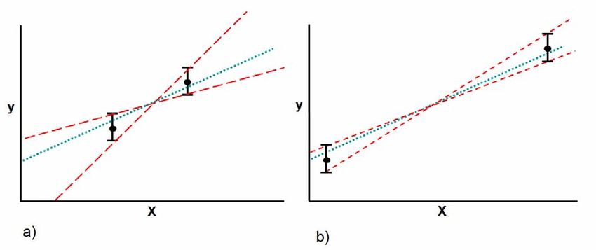
aerospace testing, MDOE practitioners recognize that direct operating costs and cycle time are proportional to the
volume of data acquired and therefore seek to organize experimental investigations around the smallest volume of
data that is still ample to achieve technical objectives.2 Likewise, quality—traditionally assessed in terms of
variability in the data—is regarded differently in an MDOE experiment.3,4 Low variability in the raw data is not
sufficient to assert high quality in an MDOE experiment. From the MDOE perspective, quality is assessed in the
context of minimized inference error risk. There must be a demonstrably high probability that the conclusions of the
study are correct, which places a strong emphasis on uncertainty assessment. This focus on quantifying uncertainty,
coupled with an emphasis on minimizing data volume requirements, made the MDOE method a likely candidate for
evaluating the debris impact assessment models developed in support of RTF activities.

                       IV.     Preliminary MDOE Screening Experiment Designs
    Four sources of uncertainty in estimating the thermal and structural reentry loads were identified. These are
    1) Model verification errors: Errors due to improper modeling of the underlying behavior of the system.
          These errors occur when the relationship between dependent system response variables and independent
          input variables is imperfectly understood. The computer code may accurately represent the mechanism that
          is programmed, but verification errors will occur if that mechanism is incorrect. Verification tests for
          modeling errors rather than coding errors.
    2) Model validation errors: Errors due to “bugs” in the software that cause improper results of calculations
          even when the relationships that are specified for coding represent the true underlying behavior of the
          system under study. These are coding errors, not modeling errors.
    3) Errors due to independent variable uncertainty: Even if the code is validated and verified, its output can
          only be as good as its input. The TPS cavity geometry variables are imperfectly known. This is due to
          ordinary experimental error in measuring them, and also because they are modeled with idealized
          rectangular “shoebox” geometries that are only approximations to the true geometry. Uncertainty in the
          independent variable specifications translates into uncertainty in the model response predictions.
    4) Lack of Fit (LOF) errors in estimating response surface models (RSM): In order to facilitate
          independent variable error propagation, it is convenient to represent the complex reentry load models with
          simpler polynomial response functions. This simplification introduces a source of error known as lack of fit
          error.
    While MDOE methods could be used to develop low-cost, high-quality model validation and verification
experiments, validation and verification considerations5 were beyond the scope of the current activity. The
computer codes developed by the United Space Alliance and the Boeing Company team for the NASA Orbiter
Project Office were assumed to have been sufficiently validated and verified that reentry load estimates made with
those codes adequately represented the true loads that would be experienced by the Orbiter on reentry. That is,
validation and verification errors were assumed to be negligible. The current effort focused on the propagation of
input variable uncertainty, including considerations of LOF errors associated with polynomial models that were
developed to facilitate the error propagation calculations.
    MDOE computational experiments were designed for each of 33 body point zones on the Orbiter’s windward
side. Theses zones are shown in Fig. 1. Initially, a series of two-level full factorial screening experiments were
designed, executed, and analyzed to rank order independent variables by their correlation with response variables of
interest, in order to identify variables with sufficiently small influence on the responses to justify dropping them
from further consideration. Eliminating irrelevant factors from detailed consideration is an important quality and
productivity step. It is important for productivity because the cases that must be run to fit a given order of
polynomial grows rapidly with the number of independent variables in the model, with attendant growth in
computational time and costs. A full dth-order polynomial model in k independent variables features p parameters,
where

                                                     p=
                                                          (d + k )!                                                  (1)
                                                            d !k !
    The test matrix must include at least one data point for each parameter in the model, and generally some
additional degrees of freedom are desirable beyond this minimum to allow an assessment of uncertainty in addition
to fitting the data. For a full third-order polynomial function in 10 variables as originally contemplated for this study
d = 3, k = 10, and by Eq. (1), p = 286. Since two of the variables were two-level categorical factors for which
quadratic and cubic terms are not necessary, there were actually only 269 points required to fit a third-order model

                                                         4
                                 American Institute of Aeronautics and Astronautics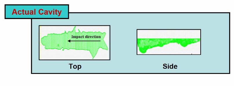
in the original 10 variables. With 20 residual degrees of freedom specified to assess uncertainty, and 15 additional
confirmation points, the original planned scale of the experiment was 269 + 20 + 15 = 304 points.
    The preliminary screening experiments justified the elimination of three variables initially identified as
candidates for more detailed investigation. The cavity exit angle was eliminated because the screening experiment
revealed that over the relatively narrow interval that experience dictated this variable ranges in practice (70° to 80°),
the regression coefficient was not large compared to the uncertainty in estimating it. It was therefore not possible to
resolve a difference between this coefficient and zero with the level of confidence (99%) adopted as criterion in this
experiment. A constant exit angle of 75° was therefore modeled, with no substantive loss in predictive power.
    Lateral and longitudinal coordinates were eliminated after anomalous behavior in the screening experiment lead
to further investigations that showed it was not possible to specify arbitrary cavity location coordinates due to the
discrete distribution of Shuttle body points. In an experiment design featuring X and Y cavity centroid coordinates,
the underlying code computed responses for the nearest Shuttle body point and assigned them to the coordinate
specified in the test matrix, notwithstanding the fact that the specified coordinates were not the coordinates for
which the response was computed. Since this would produce a false relationship between location coordinates and
response predictions, the detailed investigations were conducted for a specified, representative body point within
each zone. The option was reserved to model multiple body points within a zone if within-zone spatial response
variation was later deemed to be of special interest.
    A full third-order polynomial function in seven variables instead of 10 as originally contemplated for this study
requires a minimum of 120 points by Eq. (1). Since again two of the variables were two-level categorical factors for
which quadratic and cubic terms are not necessary, only 104 points are required to fit a third-order model in the
retained seven variables. Twenty residual degrees of freedom were added to assess uncertainty, so 124 points were
specified to fit the response surface models. There were 15 additional confirmation points for a total of 139 points
that were specified for each body point zone, down from the 304 points required for 10 variables. The savings of
165 case runs is realized for each of the 33 body point zones, a total of 5,445 cases that did not have to be run. Each
case required an average of approximately 45 minutes to run, with eight such cases typically run in parallel. The
savings of 5,445 cases therefore translates into more than 500 hours of CPU time that were saved. The actual wall-
clock savings were considerably greater, since the 45 minutes per run does not include the considerable time
required to prepare inputs for each run and other activities that consume time in addition to the CPU time of the case
runs.
    Eliminating candidate variables in a preliminary screening experiment can reduce the computer resources
required in a computational experiment, as shown. It can also improve quality, by reducing the uncertainty in
predictions made by response surface models developed from such experiments.
    The prediction variance of a polynomial regression model varies from one combination of independent variables
to another, but across all n points used to fit the model, the average prediction variance is as follows6

                                                  n

                                                 ∑ Var( yˆ )i
                                                                    pσ 2
                                                 i =1
                                                                =                                                    (2)
                                                        n            n

where p is the number of terms in the model and σ represents the standard error in the response variable. This result
holds for any model that is linear in the coefficients, including polynomial models of any order. Note that while σ
cannot be empirically determined from replicated data in a computational experiment as it can be in a physical
experiment, the response estimates have uncertainty nonetheless, and σ is a measure of that uncertainty, however it
is determined in practice.
    Equation (2) indicates that the average prediction variance increases linearly with the number of terms in the
model, so there is potential to reduce the average prediction variance simply by reducing the number of model
terms. This is because each term carries with it some contribution to the total uncertainty in the model prediction. As
Eq. (1) shows, reducing the number of variables to be fitted with a polynomial response function results in a rapid
reduction in the number of terms required for the model, and thus a rapid reduction in prediction uncertainty for
models developed by fitting a given number of data points. Alternatively, reducing the number of independent
variables can lead to the same prediction uncertainty with substantially fewer data points used to fit the response
model.
    Based on the screening experiment results, an experiment was designed to acquire data to fit a third-order
response model in seven independent variables. These variables are noted in Table 1.

                                                         5
                                 American Institute of Aeronautics and Astronautics
Table 1. Independent variables in response surface modeling experiments.

                                        Variable          Units        Low    High
                                    Cavity Length          in.          2      10
                                    Cavity Width           in.         1.4      4
                                    Cavity Depth           in.         0.1     0.6
                                    Entry Angle           deg.          10     60
                                    Sidewall Angle        deg.          10     87
                                    Baseline Heating                   Low   Nominal
                                    BLT Time               sec.        900    1200

                   V.    MDOE Experiment Designs for Response Surface Modeling
    MDOE response surface experiments were designed for each of 33 body point zones in Fig. 1. A case matrix was
developed for each of the 33 experiments, consisting of 124 unique combinations of the seven independent variables
in Table 1. The USA/Boeing computer codes were used to generate responses previously noted for each of these
variable combinations, plus 15 more that were held in reserve as confirmation points to test the models.
    To develop the test matrix for an MDOE experiment, the total number of points must be determined as described
above, and then specific points must be selected. While not generally taken into account in the design of test
matrices for aerospace research, the selection of points (not just the number of points) is an important determinant of
the quality of experimental and computational research results. Figure 2 illustrates the concept for a simple first-
order function of one variable.
    For an experiment as simple as the one illustrated in Fig. 2, the order of the model, d, is 1 and the number of
variables, k, is 1, so that Eq. (1) reminds us of the familiar fact that two points are required to fit a straight line.
Figure 2 illustrates how the uncertainty in the coefficient estimates for this model—the slope of the straight line and
the intercept—depend on the selection of two points used to fit the straight line. In this case the points that are
farther apart give a more satisfactory result than points that are closer together. This is because each point has some
uncertainty associated with it, and this uncertainty allows a range of slope and y intercepts to be consistent with the
data. This range is more restricted for one data set than another in Fig. 2.
    The term “inference space” is used to denote a k-dimensional space in which each axis corresponds to one of the
independent variables. Each site in the inference space represents a unique combination of independent variable
levels. Figure 2 illustrates the effect of site selection in a simple one-dimensional inference space. The phenomenon
illustrated in this figure for a simple first-order function of one variable is completely general. It applies to RSM
experiment designs no matter how complex the response function or how many variables are in the model. Much of
the quality enhancement of MDOE RSM experiment designs is achieved by optimizing site selections in different
ways to optimize results by various criteria.
    For the RSM experiments developed in this study, a D-optimal design strategy was implemented, in which the
points are chosen to minimize the variance associated with the estimates of model coefficients. Standard references
describe the D-optimal algorithm in detail,7,8 but modifications to the method are discussed here that were needed to
accommodate certain constraints among the independent variables in this problem.
    Consider first the design matrix, X. The design matrix is an extension of the test matrix. It has rows for each
point in the design just as a conventional test matrix does, but it also has columns for every term in the response
model, including the intercept term. The design matrix for this experiment therefore has 104 columns and 124 rows.
    The covariance matrix, C, is a (p × p) square matrix computed by pre-multiplying the design matrix by its
transpose, inverting the product, and multiplying each element of the resulting matrix by the unexplained variance of
the residuals, σ2:

                                                   C = (X′X ) σ 2
                                                                  −1
                                                                                                                    (3)

                                                         6
                                 American Institute of Aeronautics and Astronautics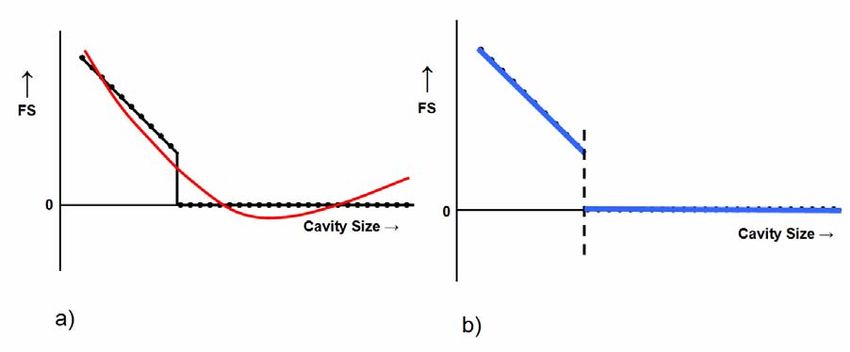
It can be shown that the diagonal elements of the covariance matrix represent the variance in estimates of the
regression coefficients. That is, the variance in the ith regression coefficient, βi is simply:

                                                     Var (β i ) = Cii                                                (4)

   To minimize the uncertainty in the regression coefficients, we must minimize the determinant of the covariance
matrix. This minimizes the confidence ellipsoids for each regression coefficient, the multidimensional equivalent of
minimizing confidence intervals about a measured data point. The D-optimal design algorithm selects the subset of
points to do this from a candidate points list.

A. D-Optimal Candidate Point List
    A candidate point list consists of a large number of potential points (typically thousands for an experiment of this
complexity), that satisfy certain criteria. Specialized software routines identify the candidate points automatically.
One such algorithm9 starts with a point selected at random from within the inference space. Subsequent points are
picked at random and retained if they increase the rank of the design matrix corresponding to a proposed regression
model that is specified at the beginning of this process. That is, points are retained if they do not feature linear
relationships among the columns of the design matrix constructed from points selected so far. This process is
continued until a full rank design matrix is obtained—one with as many unique rows (p) as columns and with no
linear dependence among any of the columns. This ensures that at least one full rank design matrix is available from
the candidate point set, which is necessary to determine the model coefficients by linear regression. Additional
points necessary to meet a total point count specified at the start of the process (in order to satisfy precision
requirements, for example) are then simply selected at random to provide broad coverage within the inference space.
    While design points chosen by this process will generally yield well-formulated regression models, not all of
these points necessarily represent physically realizable cavity geometries. This is because entry angles must exceed
a certain depth-dependent minimum to ensure realizable cavity floor lengths, and side angles must exceed a certain
depth-dependent minimum to ensure realizable cavity floor widths. These constraints form a concave hull within the
design space, outside of which all points are infeasible. Therefore, a significant departure from this D-optimal point
selection process had to be developed to accommodate these constraints on cavity geometry.
    Figure 3 illustrates the cavity geometry leading to the following equations governing these constraints:

                                                 ⎡   D        D ⎤
                                      ξL = L − ⎢           +         ⎥ − LB ≥ 0                                     (5a)
                                                 ⎣ tan (α ) tan (β ) ⎦

                                                        ⎡ 2D ⎤
                                           ξW = W − ⎢          ⎥ − WB ≥ 0                                           (5b)
                                                    ⎣ tan (φ ) ⎦

where ξL and ξw are zero when the constraints are just satisfied. If these values are less than zero, the constraints are
not met. If they are positive but relatively small, the constraints are satisfied but the point is said to be “near the
constraint boundary.” The minimum length and width of the bottom of each cavity, LB and WB, were each selected to
be 0.5 inch.
    Initially, points with negative values of either ξL or ξW were simply dropped. Unfortunately, this did not
completely address the problems with this design approach because there were also too few “near constraint” points.
This would mean that smaller cavities were not likely to be modeled as well as larger cavities. It was therefore
necessary not only to eliminate “out of constraint” points but also to add “near constraint” points.
    To ensure a large number of candidate points near the constraint boundaries as needed for good fits in that part
of the inference space, 2000 additional points were selected by a maximal distance algorithm that picks points as far
away from each other in the inference space as possible. This has the effect of “filling holes” in the inference space
by forcing a certain fraction of the points into the near-constraint region. Points were eliminated for which either
ξL < 0 or ξW < 0. This added some additional points near the boundary, and also ensured a generally uniform
distribution of candidate points throughout the seven-dimensional inference space.
    A number of additional points guaranteed to be close to the constraint boundary were then added in the
following way: A total of 50,000,000 points randomly distributed within the inference space were generated. All of

                                                         7
                                 American Institute of Aeronautics and Astronautics
these points for which both ξL and ξw were greater than 0 and less than 0.1were retained. Only 278 such points were
identified. These were added to the candidate point list. These points were selected via an algorithm written by
Wayne Adams of Stat-Ease, Inc., to run in the “R” statistical computing language. The Adams algorithm was used
in the same way to generate a further 772 points defined as “near” points. Near points feature values of ξL and ξw
greater than 0.1 and less than 0.5. This again assured a good representation within the candidate point list of points
that were in the region moderately close to the constraint boundary. The process of adding points within specified
ranges of ξL and ξw while eliminating points with negative values of those variables resulted in a final candidate
point list of 2,507 points. These points all satisfied the constraints of Eq. (5), provided good coverage (few “holes”)
throughout the seven-dimensional inference space, and concentrated points near the constraint boundary as
necessary to achieve as good a result with small cavities as with large cavities. The final set of design points was
selected from this list by the D-Optimal selection process we now describe:
B. D-Optimal Point Selection
The 124 points necessary to produce each RSM case matrix for this study were all drawn from the 2,507
candidate points created as described above. (Fifteen additional conformation points were selected at random,
subject to the constraints in Eq. (5).) The algorithm for selecting the points to fit the models begins by picking the
candidate point with the largest Euclidean norm as the first design point. This is the point that is the farthest from the
center of the design space. Figure 2 illustrates why points far from the center are desirable.
Each subsequent design point is selected to minimize the determinant of the covariance matrix in Eq. (3) while
increasing the rank of the design matrix. When a full rank design matrix has been constructed, the remaining points
in the candidate list are evaluated through a series of exchange steps to see if substituting them for points
provisionally in the design will result in an improvement.
The process begins with a one-point exchange. The point in the candidate list that decreases the determinant of
the covariance matrix the most is added to the design. The point in this augmented design that increases the
determinant of the covariance matrix the most is then dropped from the design and placed back in the candidate list.
One-point exchange steps are continued until there is no improvement in the model or until every candidate point
has been evaluated. A series of two-point exchanges then begins, in which the pair of points drawn from the
candidate list that decreases the determinant of the covariance matrix the most is added, and the pair of points from
the augmented model that increases the determinant of the covariance matrix the most is deleted. This process is
repeated with more and more points in the exchange until typically 5-point to 10-point exchanges have been
performed. Each step is taken to decrease the determinant of the covariance matrix the most by adding points, then
increase it the least by dropping an equal number of points from the design.
The entire process is repeated a number of times (typically one to 10 times), each with a different randomly
selected start point. The design with the smallest covariance matrix determinant is retained as the final design. Each
experiment designed for this study involved four such replications.
To see the effect of these changes in the experiment design, consider the “hat matrix,” H, which derives its name
from the fact that a vector of individual response measurements, y, can be transformed into a vector of
corresponding response predictions, “y-hat,” as follows:
yˆ = Hy (6)
It can be shown that the variance in predicted responses is likewise related via the hat matrix to the variance in
individual response measurements, σ 2, as follows:
Var(yˆ ) = Hσ 2 (7)
The hat matrix is a function only of the design matrix:
H = X(X′X ) X′
−1
(8)
The standard error in response predictions is just the square root of the prediction variance:
σ ŷ = X ( X′X ) X′σ
−1
(9)
8
American Institute of Aeronautics and AstronauticsEquation (9) tells us that the uncertainty in predictions made at the points used to fit the model only depends on
two things, the intrinsic variability in the response estimates and the design of the experiment (i.e., the model being
fit and the selection of independent variable levels in the test matrix). Since the researcher has complete control over
X, there is considerable latitude for improving the quality of response predictions by optimizing the design for this
purpose, and this is a major mechanism by which MDOE experiment designs improve the quality of research results.
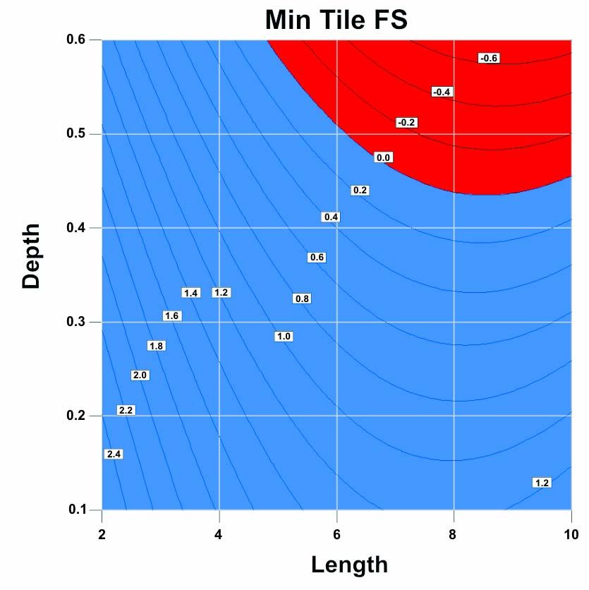
Equation (9) is especially useful because, for a unit standard deviation in response measurements, it allows us to
know the distribution of unit standard prediction errors even before the experiment is executed. By setting σ = 1, we
can use graphical representations of Eq. (9) to compare candidate experiment designs as in Fig. 4, where the
distribution of unit prediction standard errors is displayed for two variations on the experiment design discussed
above. The distributions on the left and on the right in Fig. 4 correspond to designs with different numbers of
parameters. The reduction in average prediction variance reflects Eq. (2). These distributions of unit standard
prediction errors allow rapid and convenient comparisons among candidate MDOE experiment designs. They can be
displayed as a function of any two of the independent variables at a time, with the remaining variables held at
specifiable levels. Changing the variables that are plotted and the levels of the other variables provides insight into
the robustness of the experiment design. We seek designs for which the distribution of standard prediction errors is
as low and as uniform as possible.
C. Variable Selection and Model Building
After identifying over 2500 D-optimal candidate points that each satisfied all factor constraints and were all
distributed optimally throughout the inference space, with points near the constraint boundaries and other points
distributed to minimize large holes in the inference space, the D-Optimal selection process identified a 124-point
subset of these candidate points that most minimized the determinant of the covariance matrix for a third-order
polynomial. This set of points is the smallest number that will fit the polynomial and still minimize uncertainty in
the regression coefficients, while allowing up to 20 additional lack of fit degrees of freedom to fit unanticipated
higher-order complexities in the data.
For each of the 33 body point zones, the USA/Boeing code was executed for each of 124 unique combinations of
variables from Table 1. Various thermal and structural reentry load responses were recorded for each such case.
Stepwise procedures were used to develop third-order polynomial models for each response variable as a function of
all seven independent variables. These procedures are intended to identify a subset of the 104-terms in a full third-
order polynomial in five numerical variables and two 2-level categorical variables, by discarded statistically
insignificant terms from the full model. These are terms that are not large enough to be distinguished from zero with
high confidence.
While the number of terms eliminated from the regression models in this way varied from response variable to
response variable, and to a lesser degree from body point zone to body point zone, typically only around a quarter of
the terms were retained. These were mostly first-order and second-order terms, with a few mixed cubic terms and an
occasional full cubic term retained. This suggests that the responses being modeled were predominantly second
order, with some slight additional complexity that could be addressed with a few higher-order terms. The
elimination of so many terms enhanced the quality of predictions by Eq. (2), and also brought a certain level of
clarity to the response models by reducing the clutter associated with superfluous terms in the response model. The
truly important terms provided insight into which factors most significantly influenced each thermal and structural
reentry load response.
Three stepwise procedures employed in various combinations in the model-building process will now be
described briefly. These are known as (1) “Forward Selection,” (2) “Backwards Elimination,” and (3) “Stepwise
Regression,” which is actually a combination of the first two methods. Standard textbooks on regression
analysis6-8,10 can be consulted for a more detailed description of these methods, which are outlined here.
Forward Selection begins by assuming that only the intercept term is in the model. It then provisionally adds
the one term that has the highest correlation with the response. An analysis of variance (ANOVA) is conducted for
this two-term model. If the explained variance is increased by a specified threshold amount (indicating low
probability that the added term is insignificant), the term is retained and the forward selection process continues. The
next term to be provisionally entered is the one that has the highest correlation with the response after correcting for
first term entered. This is called a “partial correlation,” and an ANOVA on this model indicates the probability that
this term makes a significant change to the explained variance of the model. If so, this term is retained. The process
continues until either all terms from the initial model have been included, or until the most significant remaining
term does not cause enough of a change in the explained variance to satisfy the entry criterion.
Backward Elimination is similar to forward selection except that the process attempts to identify terms for the
final model by working in the opposite direction. The backward elimination method begins with all terms from the
9
American Institute of Aeronautics and Astronauticsinitial model included. The term having the weakest correlation with the response is provisionally rejected, and the
impact on the explained variance of the model is assessed by ANOVA. If the rejection of this term produces a
significant reduction in the variance explained by the model, it is retained and the process stops. Otherwise, the
process continues until no terms in the model can be rejected without causing a significant reduction in the variance
explained by the model, or until the only remaining term is the intercept.
Stepwise Regression is a combination of forward selection and backward elimination. It begins as a forward
selection process and continues until the model contains the intercept and two regressors. Now backward
elimination is applied to the three-term model, eliminating each regressor in turn to assess the reduction in the
model’s explained variance via ANOVA. When the backward elimination step is finished, the forward selection
process is resumed with whichever remaining term causes the most significant increase in the explained variance. If
such a term increases the explained variance by a user-specified threshold amount, it is retained and the backward
elimination is initiated on the new model. This is continued until there are no candidate regressors significant
enough to enter the model and none in the model that are so weak that they can be eliminated with no significant
effect.
Proponents of stepwise regression note that the backward elimination step protects against multicollinearity, a
condition that exists when two or more regressors are highly correlated and therefore do not each contribute
independently to the model. If two regressors are highly correlated, adding one of them to the model may render the
first one superfluous. In such a case it is better to eliminate that term.
It is common to apply more than one stepwise procedure to the same data set. For example, in this study
backward elimination was applied first, to give all model terms a chance to be included. Stepwise regression was
then applied to the surviving model terms, with one more applications of backward elimination as a finishing step, to
reject the occasional high-order term that survives the first two applications without contributing significantly to the
model.
To summarize, we have applied stepwise regression procedures to develop response surface models from a
volume of data ample for this purpose but no larger, drawn from a large list of candidate data points that all satisfied
complex constraints among the independent variables. The large candidate point list was designed to include a
substantial fraction of candidates in the region of constraint boundaries in the seven-dimensional inference space,
while providing uniform coverage throughout the rest of the inference space. This ensured a good representation for
small cavities as well as large cavities. Points selected from the candidate list consisted of a relatively small subset
with good D-optimal properties; that is, with a distribution within the inference space that minimized the uncertainty
in regression coefficients by minimizing the determinant of the covariance matrix associated with the proposed
third-order polynomial model. In short, many steps were taken through the MDOE process to ensure that the
polynomial response models would faithfully reproduce the discrete values generated by the underlying debris
impact assessment codes.
Figure 5 is a schematic representation of the relationship between a set of such discrete code outputs and the
polynomial response model chosen to represent them. The difference between each output of the underlying debris
impact assessment code and the corresponding polynomial response model prediction is a residual which gives some
measure of how well the polynomial model represents the underlying code. Figure 6 displays the residuals for a
representative example—structure temperature for body point zone 1602. The standard deviation of these residuals
is 1.2° F. There are a total of 139 residuals in Fig. 6, of which the 124 blue points are model residuals and the 15 red
points are confirmation point residuals. The model residuals might be expected to be relatively small because the
least-squares fitting algorithm distributes the regression coefficients to ensure that this is so. The fact that the
confirmation points residuals are of the same order as the model residuals suggests that the model results are
transferable to points other than those for which the model was developed, implying a certain degree of robustness
in the polynomial response model.
Models developed by these stepwise procedures were subjected to a wide array of model adequacy tests. The
residuals were examined graphically as a function of predicted value, run number, and independent variable level to
look for tell-tale patterns that would reveal a poor fit. Numerous model adequacy metrics were computed, including
R-squared, adjusted R-squared, and Predicted R-squared statistics. The leverage of each point was computed as was
its Cook’s distance, two statistics indicating the susceptibility of the model to outliers. The magnitude of the
residuals was examined to determine if the prediction accuracy was acceptable. The distributional properties of the
residuals were also examined, to look for evidence of systematic lack of fit. Only after passing this battery of quality
assurance tests was a polynomial model declared to adequately represent the underlying USA/Boeing code. It was
then deemed suitable to use for propagating errors in the specification of cavity geometry into uncertainty in the
thermal and structural reentry load estimates.
10
American Institute of Aeronautics and AstronauticsVI. Error Propagation
The purpose of approximating the underlying USA/Boeing debris impact assessment code with polynomial
response functions was to facilitate error propagation, as will be discussed in this section. Geometry estimates
describing the size and shape of debris impact cavities necessarily suffer from some degree of uncertainty. In
addition to the usual experimental error in estimates of any experimental variable, there is also a significant
component of uncertainty attributable to the approximations that are made in representing the cavities in the
underlying damage assessment codes. Figure 7 provides an example of such an approximation.
Because of the inevitable error associated with these cavity size and shape approximations, it is important to
understand how this error translates into uncertainty in the response estimates. That is, we wish to know how much
uncertainty is introduced into the estimates of such system responses as structure temperature and structural margin
of safety by the fact that the cavity size and shape estimates are imperfect. This is the central question for which the
polynomial response model approximations were developed, as will be described in more detail in this section.
Consider a simple function of two random variables, x1 and x2. Such a function can be represented as a Taylor
series expansion about the means of those variables, which to first order is as follows:
∂y ∂y
y ( x1 , x2 ) = y ( x1 , x2 ) + ( x1 − x1 ) + ( x2 − x2 ) (10)
∂x1 ∂x2
or
∂y ∂y
y− y = ( x1 − x1 ) + ( x2 − x2 ) (11)
∂x1 ∂x2
Following Coleman and Steele,11 imagine now that there are n measurements of x1 and x2, from which n
estimates of y(x1, x2) have been computed. We know the uncertainties in x1 and x2, and we wish to propagate these
uncertainties into an estimate of the corresponding uncertainty in y.
For all n sets of data, square the terms on the left and right side of Eq. (11), and average the squared values.
2 2
1⎡ n 2⎤ ⎛ ∂y ⎞ 1 ⎡ n 2⎤ ⎛ ∂y ⎞ 1 ⎡ n 2⎤
⎢ ∑
n ⎣ i =1
( yi − y ) ⎥ = ⎜ ⎟ × ⎢ ∑
⎦ ⎝ ∂x1 ⎠ n ⎣ i =1
( x1i − x1 ) ⎥ + ⎜ ⎟ × ⎢ ∑ ( x2i − x2 ) ⎥
⎦ ⎝ ∂x2 ⎠ n ⎣ i =1 ⎦
(12)
⎛ ∂y ⎞⎛ ∂y ⎞ 1 ⎧ n ⎫
+2 ⎜ ⎟⎜ ⎟ × ⎨∑ ⎡⎣( x1i − x1 )( x 2i − x2 ) ⎤⎦ ⎬
⎝ ∂x1 ⎠⎝ ∂x2 ⎠ n ⎩ i =1 ⎭
By the definition of population variance, and with an obvious notational extension for the cross term on the right,
in the large n limit this becomes:
⎛ ∂y ⎞ 2 ⎛ ∂y ⎞ 2 ⎛ ∂y ⎞⎛ ∂y ⎞
σ y2 = ⎜ ⎟ σ x1 + ⎜ ⎟ σ x2 + 2 ⎜ ⎟⎜ ⎟ σ x1 x2 (13)
⎝ ∂x1 ⎠ ⎝ ∂x2 ⎠ ⎝ ∂x1 ⎠⎝ ∂x2 ⎠
The correlation coefficient for x1 and x2 is defined as
σx x
ρx x = 1 2
(14)
1 2
σx σx
1 2
so that Eq. (13) becomes
2 2
⎛ ∂y ⎞ 2 ⎛ ∂y ⎞ 2 ⎛ ∂y ⎞⎛ ∂y ⎞
σ =⎜
2
⎟ σ x1 + ⎜ ⎟ σ x2 + 2 ⎜ ⎟⎜ ⎟ ρ x1 x2 σ x1σ x2 (15)
⎝ ∂x1 ⎠ ⎝ ∂x2 ⎠ ⎝ ∂x1 ⎠⎝ ∂x2 ⎠
y
11
American Institute of Aeronautics and AstronauticsFor independent x1 and x2 the correlation coefficient is zero, and for k independent variables Eq. (15) generalizes
to
2 2 2
⎛ ∂y ⎞ 2 ⎛ ∂y ⎞ 2 ⎛ ∂y ⎞ 2
σ =⎜
2
⎟ σ x1 + ⎜ ⎟ σ x2 + " + ⎜ ⎟ σ xk (16)
⎝ ∂x1 ⎠ ⎝ ∂x2 ⎠ ⎝ ∂xk ⎠
y
It is clear from Eq. (16) why it is so convenient to represent a complex computer code as a simple low-order
polynomial function of the independent variables. The derivatives in Eq. (16) become trivial to evaluate in that case,
and since the standard deviations for all xi is assumed to be known, the corresponding response uncertainty in y is
easily computed from Eq. (16). For example, if y represents reentry structure temperature as a function of cavity
geometry variables that all have associated with them some uncertainty, then Eq. (16) can easily quantify the
uncertainty in structure temperature attributable to the cavity geometry uncertainties. Table 2 lists the uncertainty
specifications for debris impact cavity geometry variables assumed in this study.
Table 2. Uncertainty in cavity geometry variables.
Variable Specified Uncertainty Standard Error (“one σ”)
Length 3σ = 0.125 in. 0.042 in.
Width 3σ = 0.125 in. 0.042 in.
Depth 3σ = 0.125 in. 0.042 in.
Entry angle 2σ = 5° 2.5°
Sidewall angle 2σ = 5° 2.5°
Figure 8 shows a typical polynomial response surface model for structure temperature as a function of cavity
length and depth. The length and depth are displayed in coded units, where -1 and +1 correspond to the smallest and
largest values of the indicated variables for which the regression model is valid. The corresponding uncertainty in
structure temperature is displayed for the propagation of a two-sigma uncertainty in cavity geometry variables. So,
by Fig. 8, the predicted temperature for a relatively long, deep cavity would have a two-sigma uncertainty of about
±2.5° F due to the errors in cavity geometry that are presented in Table 2. It is easy to examine the impact of errors
of a different magnitude once the polynomial response and error propagation models have been created, and the
sensitivity of the response uncertainty to errors in specific geometry variables can also be easily examined.
Obviously, other insights can be obtained from response surface models of reentry loads and their corresponding
uncertainties, as will be discussed in the next section.
VII. Results and Discussion
This paper is focused on the MDOE experiment design and analysis process used in this study to quantify the
impact of cavity geometry error on estimates of thermal and structural reentry loads. Many other insights can be, and
were, achieved from the polynomial response models developed in this study. In addition to revealing interesting
patterns in the data that illuminated the underlying physical processes in play, the modeling process also revealed
certain apparent anomalies in the parametric codes upon which they were based. These patterns and apparent
anomalies are documented in detail in a comprehensive report12 prepared by the Jacobs Technology Engineering and
Science Contract Group in Houston. While a detailed exposition in this paper of all of these findings would be
redundant, we site a few representative examples that bear on the response surface modeling activity and that
therefore have some impact on the cavity geometry error propagation problem.
The coefficient of variation (CV) is a metric that describes how well a response surface function represents the
underlying process it models. It is computed by dividing the standard deviation of residuals by the mean response
over the points for which the residuals were computed. Figure 9 presents the coefficients of variation for the
response variables modeled in this study. Note the pronounced difference between coefficients of variation for the
thermal responses (blue) and the structural responses (red). The CV values for the thermal responses are less than
2%, while none of the structural response CV values are less than 4%—twice the maximum thermal CV. This
illustrates that it was much more difficult to model the structural responses than the thermal responses.
There are a number of plausible explanations for this. Some of the structural responses exhibited a certain degree
of discontinuous behavior that is difficult to model well with a low-order polynomial, for example. The tiles are
believed to remain in plane until stressed to a certain threshold level, beyond which they “pop” into an out-of-plane
12
American Institute of Aeronautics and Astronauticsconfiguration. In mathematical terms, the out-of-plane-deflection (OOPD) functions are not continuous with
continuous derivatives, conditions that must be met to represent them well with a Taylor series corresponding to the
polynomial models we have tried to fit. This may explain why the two OOPD responses in Fig. 9 have the greatest
coefficients of variation—about 14% for the Mach 25 to Mach 4 regime of the reentry trajectory and about 8% for
the terminal area energy management regime. These are four to seven times greater than the largest thermal CV
value.
The CV for tile factor of safety (FS) was twice as large as the largest thermal CV, a fact that may be attributable
to a difference in behavior as the cavity exceeds the threshold level beyond which the RTV bonding fails and the tile
is lost. The true tile FS is believed to degrade as debris impact loads increase, until this threshold is reached. Beyond
that point, the tile FS is essentially undefined—the concept of factor of safety for a tile that is already lost is
meaningless. Unfortunately, the underlying code reports a numerical value of zero for FS in such circumstances,
rather than “Not Applicable” or some other such non-numeric descriptor. The result of this is represented
schematically in Fig. 10.
The red curve on the left of Fig. 10 represents the best third-order polynomial approximation to the data points
that track the true behavior, represented by the black line. The discontinuity results in a very poor fit over the full
range of cavity sizes. For example, in an effort to model both the zero and non-zero FS regions, the response model
underestimates tile FS where it has meaningful values. This is followed by a region in which the tile has already
failed, but the model is reporting non-zero FS values. Beyond that, the modeled FS values go negative, which is
physically non-realizable. Finally, a cavity size is reached beyond which the model predicts that as the cavity size
increases, the tile FS increases. Obviously these are all nonsensical results, caused by an attempt to use a single,
simple polynomial model to span two regions in which radically different physical processes are in play.
The blue curve on the right of Fig. 10 represents how different response models would be fitted to the two
regions if the boundary between them were known. For the FS = 0 region, the polynomial response function is a
trivial 0th-order function (intercept only); viz., y = b0, where b0 = 0. Where FS is not zero, a conventional polynomial
model would be expected to fit the data adequately.
The problem of finding the boundary between meaningful and meaningless FS values is not straightforward. One
can simply fit the FS values over cavity dimensions known to be small enough for the tile not to fail, but there is
always a danger of being too conservative in this approach. Generally, the behavior right up to the boundary is of
interest. An alternative approach, proposed as a result of this study, is to design a series of MDOE experiments. In
the first, distribute points throughout the entire inference space without regard to whether FS response values are
meaningful or not. Analyze the data, noting where the response surface goes below some threshold value. Figure 11
is an example of such a result, where the red and blue regions denote the boundary where FS = 0. (Note that other
boundaries might be superior for this type of analysis, such as the boundary beyond which the FS values decline
below 1, the lowest level attributable to an undamaged tile, or below 1.4, the acceptable flight threshold.) Design a
second experiment in which the data points are distributed only in the region where preliminary results indicate FS
values of actual interest. Fit the data in this region. It may be necessary to iterate more than once, but with
experience it should become possible to satisfactorily identify the boundary.
In the present study, tile FS models were simply not attempted in body point zones with an excessive number of
zero-value FS points (where “excessive” was defined as “five or more”). However, it is still possible that the FS
responses were sufficiently discontinuous for the cases in which zero-FS values were modeled, that the low-order
polynomial models were still inadequate to properly capture all of the variation in FS over these regions. We
conclude that when there are two regions in which the underlying physics is radically different, it is necessary to
first identify the boundary between those regions, and then fit separate models in each of them.
Certain anomalies were discovered in the course of building the structural response polynomial models that have
been attributed at least in part to the behavior of the Stress Assessor Tool. The Stress Assessor Tool failed to
produce estimates of structure margin of safety and tile out of plane displacement (OOPD) for 12 of the 33 body
point zones. Adequate third order polynomial fits could not be achieved for structure margin of safety in four body
point zones despite data having been produced by the Stress Assessor Tool, and likewise adequate Mach 25 to Mach
4 OOPD models could not be generated in four other zones. TAEM OOPD models could not be generated in five
additional body point zones.
Further investigation revealed certain anomalies within the Stress Assessor Tool. For example, in some body
point zones there were no changes in structural responses despite large changes in input variables. This caused some
of the structure response polynomial models to have only one or two significant terms, as there was not enough
change attributable to other factors for the regression coefficients for those terms to be resolvable from zero. In
addition, in certain other zones structure margins of safety were sometimes larger for damaged tile than undamaged
tile. This is clearly a suspect result. There have been a number of improvements in the Stress Assessor Tool and
13
American Institute of Aeronautics and AstronauticsYou can also read