Scalable Scene Flow from Point Clouds in the Real World - arXiv
←
→
Page content transcription
If your browser does not render page correctly, please read the page content below
Scalable Scene Flow from Point Clouds in the Real World
                                                         Philipp Jund         ∗,1 ,   Chris Sweeney   ∗,2 ,   Nichola Abdo 2 , Zhifeng Chen 1 , Jonathon Shlens            1
                                                                                                      1                   2
                                                                                                          Google Brain,       Waymo
                                                                                                {abdon,cjsweeney}@waymo.com

                                             Abstract— Autonomous vehicles operate in highly dynamic                   correspondence exists between LiDAR returns from subse-
                                         environments necessitating an accurate assessment of which                    quent time points. Instead, one must rely on semi-supervised
                                         aspects of a scene are moving and where they are moving to. A                 methods that employ auxiliary information to make strong
                                         popular approach to 3D motion estimation, termed scene flow,
                                                                                                                       inferences about the motion signal in order to bootstrap
arXiv:2103.01306v4 [cs.CV] 13 Sep 2021

                                         is to employ 3D point cloud data from consecutive LiDAR scans,
                                         although such approaches have been limited by the small size of               annotation labels [10], [11]. Such an approach suffers from
                                         real-world, annotated LiDAR data. In this work, we introduce a                the fact that motion annotations are extremely limited (e.g.
                                         new large-scale dataset for scene flow estimation derived from                400 frames in [10], [11]) and often rely on pretraining a
                                         corresponding tracked 3D objects, which is ∼1,000× larger                     model based on synthetic data [12] which exhibit distinct
                                         than previous real-world datasets in terms of the number of
                                         annotated frames. We demonstrate how previous works were                      noise and sensor properties from real data. Furthermore,
                                         bounded based on the amount of real LiDAR data available,                     previous datasets cover a smaller area, e.g., the KITTI scene
                                         suggesting that larger datasets are required to achieve state-                flow dataset covers 1/5th the area of our proposed dataest.
                                         of-the-art predictive performance. Furthermore, we show how                   This allows for different subsampling tradeoffs and inspired
                                         previous heuristics for operating on point clouds such as                     a class of models that are not able to tractably scale training
                                         down-sampling heavily degrade performance, motivating a new
                                         class of models that are tractable on the full point cloud. To                and inference beyond ∼10K points [7], [8], [9], [13], [14],
                                         address this issue, we introduce the FastFlow3D architecture                  making the usage of such models impractical in real world
                                         which provides real time inference on the full point cloud.                   AV scenes which often contain 100K - 1000K points.
                                         Additionally, we design human-interpretable metrics that better                  In this work, we address these shortcomings of this field
                                         capture real world aspects by accounting for ego-motion and
                                         providing breakdowns per object type. We hope that this                       by introducing a large scale dataset for scene flow geared
                                         dataset may provide new opportunities for developing real                     towards AVs. We derive per-point labels for motion estima-
                                         world scene flow systems.                                                     tion by bootstrapping from tracked objects densely annotated
                                                                                                                       in a scene from a recently released large scale AV dataset
                                                                   I. I NTRODUCTION                                    [15]. The resulting scene flow dataset contains 198K frames
                                                                                                                       of motion estimation annotations. This amounts to roughly
                                                                                                                       ∼1,000× larger training set than the largest, commonly used
                                            Motion is a prominent cue that enables humans to navi-                     real world dataset (200 frames) for scene flow [10], [11].
                                         gate complex environments [1]. Likewise, understanding and                    By working with a large scale dataset for scene flow, we
                                         predicting the 3D motion field of a scene – termed the scene                  identify several indications that the problem is quite distinct
                                         flow – provides an important signal to enable autonomous                      from current approaches:
                                         vehicles (AVs) to understand and navigate highly dynamic
                                                                                                                              •   Learned models for scene flow are heavily bounded by
                                         environments [2]. Accurate scene flow prediction enables an
                                                                                                                                  the amount of data.
                                         AV to identify potential obstacles, estimate the trajectories of
                                                                                                                              •   Heuristics for operating on point clouds (e.g. down-
                                         objects [3], [4], and aid downstream tasks such as detection,
                                                                                                                                  sampling) heavily degrade predictive performance. This
                                         segmentation and tracking [5], [6].
                                                                                                                                  observation motivates the development of a new class
                                            Recently, approaches that learn models to estimate scene
                                                                                                                                  of models tractable on a full point cloud scene.
                                         flow from LiDAR have demonstrated the potential for
                                                                                                                              •   Previous evaluation metrics ignore notable systematic
                                         LiDAR-based motion estimation, outperforming camera-
                                                                                                                                  biases across classes of objects (e.g. predicting pedes-
                                         based methods [7], [8], [9]. Such models take two con-
                                                                                                                                  trian versus vehicle motion).
                                         secutive point clouds as input and estimate the scene flow
                                         as a set of 3D vectors, which transform the points from                       We discuss each of these points in turn as we investigate
                                         the first point cloud to best match the second point cloud.                   working with this new dataset. Recognizing the limitations
                                         One of the most prominent benefits of this approach is that                   of previous works, we develop a new baseline model ar-
                                         it avoids the additional burden of estimating the depth of                    chitecture, FastFlow3D, that is tractable on the complete
                                         sensor readings as is required in camera-based approaches                     point cloud with the ability to run in real time (i.e. <
                                         [6]. Unfortunately, for LiDAR based data, ground truth                        100 ms) on an AV. Figure 1 shows scene flow predictions
                                         motion vectors are ill-defined and not tenable because no                     from FastFlow3D, trained on our scene flow dataset. Finally,
                                                                                                                       we identify and characterize an under-appreciated problem
                                           ∗   Denotes equal contributions.                                            in semi-supervised learning based on the ability to predict
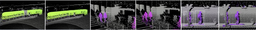
Fig. 1: LiDAR scene flow estimation for autonomous vehicles. Left: Overlay of two consecutive point clouds (green and
blue, respectively) sampled at 10 Hz from the Waymo Open Dataset [15]. White boxes are tracked 3D bounding boxes for
human annotated vehicles and pedestrians. Middle: Predicted scene flow for each point colored by direction, and brightened
by speed based on overlaid frames† . Right: Two qualitative examples of bootstrapped annotations.

the motion of unlabeled objects. We suspect the degree                     perceived tracklets. These recent datasets offer an opportu-
to which the fields of semi-supervised learning attack this                nity to propose a methodology to construct point-wise flow
problem may have strong implications for the real-world                    annotations from such data (Section III-B).
application of scene flow in AVs. We hope that the resulting                  We extend the Waymo Open Dataset (WOD) to con-
dataset presented in this paper may open the opportunity for               struct a large-scale scene flow benchmark for dense point
qualitatively new forms of learned scene flow models.                      clouds [15]. We select the Waymo Open Dataset because the
                                                                           bounding box annotations are at a higher acquisition frame
                       II. R ELATED W ORK                                  (10 Hz) than competing datasets (e.g. 2 Hz in [28]) and
A. Benchmarks for scene flow estimation                                    contain ∼ 5× the number of returns per LiDAR frame (Table
   Early datasets focused on the related problems of inferring             1, [15]). In addition, the Waymo Open Dataset also provides
depth from a single image [16] or stereo pairs of images                   ∼ 10× more scenes and annotated LiDAR frames than
[17], [18]. Previous datasets for estimating optical flow were             Argoverse [27]. Recently, [29] released a large-scale dataset
small and largely based on synthetic imagery [19], [20], [21],             with 1,000+ hours of driving data. However, their tracked
[22]. Subsequent datasets focused on 2D motion estimation                  object annotations are not human-annotated but based on the
in movies or sequences of images [23]. The KITTI Scene                     results of the onboard perception system.
Flow dataset represented a huge step forward, providing                    C. Models for learning scene flow
non-synthetic imagery paired with accurate ground truth
                                                                              There is a rich literature of building learned models for
estimates However, it contained only 200 scenes for train-
                                                                           scene flow using end-to-end learned architectures [30], [31],
ing and involved preprocessing steps that alter real-world
                                                                           [8], [7], [14], [13], [32], [25] as well as hybrid architectures
characteristics [10]. FlyingThings3D offered a modern large-
                                                                           [33], [34], [35]. We discuss these in Section V in conjunction
scale synthetic dataset comprising ∼20K frames of high
                                                                           with building a scalable baseline model that operates in real
resolution data from which scene flow may be bootstrapped
                                                                           time. Recently, Lee et al. presented an approach for predict-
[12]. Internal datasets by [24], [25] are constructed similarly
                                                                           ing pillar-level flow [25]. Whereas our model leverages a
to ours, but are not publicly available and do not offer a
                                                                           similar pillar-based architecture, we tackle the full scope of
detailed description. Recently, [26] created two scene flow
                                                                           the scene flow problem and predict point-level flow while
datasets in a similar fashion, subsampling 2,691 and 1,513
                                                                           being tractable enough for real-time applications.
training scenes from the Argoverse [27] and nuScenes [28]
                                                                              Moreover, many previous works train models on synthetic
datasets, resepectively. However, even without subsampling,
                                                                           datasets like FlyingThings3D [12] and evaluate and/or fine-
larger datasets in terms of scenes and number of points are
                                                                           tune on KITTI Scene Flow [11], [10]. Typically, these
needed to train more accurate scene flow models as shown
                                                                           models are limited in their ability to leverage synthetic data
in [26] and Figure 4.
                                                                           in training. This observation is in line with the robotics
B. Datasets for tracking in AV’s                                           literature and highlights the challenges of generalization from
                                                                           the simulated to the real world [36], [37], [38], [39].
  Recently, there have been several works introducing large-
scale datasets for autonomous vehicle applications [11], [27],                   III. C ONSTRUCTING A S CENE F LOW DATASET
[28], [29], [15]. While these datasets do not directly provide
                                                                             In this section, we present an approach for generating
scene flow labels, they provide vehicle localization data, as
                                                                           scene flow annotations bootstrapped from existing labeled
well as raw LiDAR data and bounding box annotations for
                                                                           datasets. We first formalize the scene flow problem definition.
  † Please note that we predict 3D flow, but color the direction of flow   We then detail our method for computing per-point flow
with respect to the x-y plane for the visualization.                       vectors by leveraging the motion of 3D object label boxes.
We emphasize that many details abound in the assumptions              In this work, we apply this methodology on
behind such annotations, how to calculate various trans-           the Waymo Open Dataset [15]. The dataset offers a
formations in the track labels, as well as how to handle           large scale with diverse LiDAR scenes where objects have
important edge cases.                                              been manually and accurately annotated with 3D boxes at
                                                                   10Hz. Finally, the accurate AV pose information permits
A. Problem definition                                              compensating for ego motion. We note that the method
                                                                   for scene flow annotation is general and may be used to
   We consider the problem of estimating 3D scene flow in
                                                                   estimate 3D flow vectors of the label box poses available in
settings where the scene at time ti is represented as a point
                                                                   other datasets [28], [29], [15], [40].
cloud Pi as measured by a LiDAR sensor mounted on the
AV. Specifically, we define scene flow as the collection of              IV. E VALUATION M ETRICS FOR S CENE F LOW
3D motion vectors f := (v x , v y , v z )> for each point in the
                                                                      Two common metrics used for 3D scene flow
scene where v d is the velocity in the d directions in m/s.
                                                                   are mean L2 error of pointwise flow and the
   Following the scene flow literature, we predict flow given
                                                                   percentage of predictions with L2 error below a given
two consecutive point clouds of the scene, P−1 and P0 .
                                                                   threshold [7], [24]. In this work, we additionally propose
The scene flow encodes the motion between the previous
                                                                   modifications to improve the interpretability of the results.
and current time steps, t-1 and t0 , respectively. We predict
the scene flow at the current time step, P0 in order to make
                                                                   Breakdown by object type. Objects within the AV
the predictions practical for real time operation.
                                                                   scene (e.g. vehicles, pedestrians) have different speed
                                                                   distributions dictated by the object class (Section VI-A).
B. From tracked boxes to flow annotations
                                                                   This becomes especially apparent after accounting for ego
    Obtaining ground truth scene flow from standard real-          motion. Reporting a single error ignores these systematic
world LiDAR data is a challenging task. One challenge is           differences.In practice, we find it more meaningful to report
the lack of point-wise correspondences between subsequent          all prediction performances delineated by the object label.
LiDAR frames. Manual annotation is too expensive and
humans must contend with ambiguity due to changes in               Binary classification formulation. One important practical
viewpoint and partial occlusions. Therefore, we focus on           application of predicting scene flow is enabling an AV to
a scalable automated approach bootstrapped from existing           distinguish between moving and stationary parts of the
labeled, tracked objects in LiDAR data sequences.                  scene. In that spirit, we formulate a second set of metrics
    The annotation procedure is straightforward. We assume         that represent a “lower bar” which captures a useful
that labeled objects are rigid and calculate point velocities      rudimentary signal. We employ this metric exclusively for
using a secant line approximation. For each point p0 at time       the more difficult task of semi-supervised learning (Section
t0 , we compute the flow annotation as f = ∆1t (p0 − p−1 ),        VI-C) where learning is more challenging. In particular, we
where ∆t = t0 − t-1 , p−1 = T∆ p0 is the corresponding             assign a binary label to each reflection as either moving or
point at t-1 , and T∆ is a homogeneous transformation              stationary based on a threshold, |f | ≥ fmin . Accordingly,
inferred from the track labels of the object to which the point    we compute precision and recall metrics for these binary
belongs (If there is no label at t-1 , the flow is annotated       labels across an entire scene. Selecting a threshold, fmin , is
as invalid.). This captures how a moving object may have           not straightforward as there is an ambiguous range between
varying per-point flow magnitudes and directions. Though           very slow and stationary objects. For simplicity, we select
our rigidity assumption does not necessarily apply to non          a conservative threshold of fmin = 0.5 m/s (1.1 mph) to
rigid objects (e.g. pedestrians), the high frame rate (10 Hz)      assure that things labeled as moving are actually moving.
minimizes non-rigid deformations between adjacent frames.
    In order to calculate the transformation T∆ , we compen-          V. FAST F LOW 3D: A S CALABLE BASELINE M ODEL
sate for the ego motion of the AV because this leads to               The average scene from the Waymo Open Dataset consists
superior predictive performance since a learned model does         of 177K points (Table II), even though most models [7],
not need to additionally infer the AV’s motion (most AVs are       [8], [9], [13], [14] were designed to train with 8,192 points
equipped with an IMU/GPS system to provide such informa-           (16,384 points in [14]). This design choice favors algorithms
tion). Furthermore, compensating for ego motion improves           that scale poorly to O(100K) regimes. For instance, many
the interpretability of the evaluation metrics (Section IV)        methods require preprocessing techniques such as nearest
since the predictions are now independent of the AV motion.        neighbor lookup. Even with efficient implementations [46],
We use this approach to compute the flow vectors for all           [47], increasing fractions of inference time are dedicated to
points in P0 belonging to labeled objects. Points outside the      preprocessing instead of the core inference operation.
labeled objects are assigned a flow of 0 m/s. This stationary         For this reason, we propose a new model that exhibits
assumption works well in practice, but has a notable gap           favorable scaling properties and may operate on O(100K) in
when considering unlabeled moving objects in the scene. See        a real time system. We name this model FastFlow3D (FF3D).
Section VI-C for an in depth analysis on how our model can         In particular we exploit the fact that LiDAR point clouds are
generalize to unlabeled moving objects.                            dense, relatively flat along the z dimension, but cover a large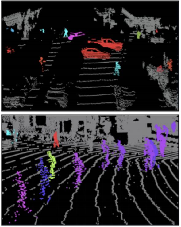
32K       100K        255K      1000K
                                  concat                                             HPLFlowNet [9]           431.1     1194.5         OOM        OOM
                                 in depth
  t0                                                                                 FlowNet3D [7]            205.2      520.7      1116.4      3819.0
                                                                                    FastFlow3D (ours)          49.3       51.9        63.1        98.1

                                                                                  TABLE I: Inference latency varying point cloud sizes. All
                                     shared                                       numbers report latency in ms on a NVIDIA Tesla P100 with
  t−1                                weights
                                                                                  batch size = 1. The timings for HPLFlowNet [9] differ from
              PointNet                Convolutional      Grid Flow   Multilayer
        (dynamic voxelization)     Autoencoder (U-Net)   Embedding   Perceptron
                                                                                  reported results as we include the required preprocessing on
                                                                                  the raw point clouds. OOM indicates out of memory.
Fig. 2: Diagram of FastFlow3D model. FastFlow3D con-
sists of 3 stages employing a PointNet encoder with dynamic                       spatial resolution. Subsequently, we use a 2D convolution
voxelization [41], [42], a convolutional autoencoder [43],                        to obtain contextual information at the different resolutions.
[44] with weights shared across two frames, and a shared                          These context embeddings are used as the skip connections
MLP to regress an embedding on to a point-wise motion                             for the U-Net, which progressively merges context from
prediction. For details, see Section V and Appendix in [45].                      consecutive resolutions. To decrease latency, we introduce
                                                                                  bottleneck convolutions and replace deconvolution opera-
area along the x and y dimensions. The proposed model is
                                                                                  tions (i.e. transposed convolutions) with bilinear upsampling
composed of three parts: a scene encoder, a decoder fusing
                                                                                  [48]. The resulting feature map of the U-Net decoder rep-
contextual information from both frames, and a subsequent
                                                                                  resents a grid-structured flow embedding. To obtain point-
decoder to obtain point-wise flow (Figure 2).
                                                                                  wise flow, we introduce the unpillar operation, which for
   FastFlow3D operates on two successive point clouds
                                                                                  each point retrieves the corresponding flow embedding grid
where the first cloud has been transformed into the co-
                                                                                  cell, concatenates the point feature, and uses a multi layer
ordinate frame of the second. The target annotations are
                                                                                  perceptron to compute the flow vector.
correspondingly provided in the coordinate frame of the
                                                                                     As proof of concept, we showcase how the resulting archi-
second frame. The result of these transformation is to remove
                                                                                  tecture achieves favorable scaling behavior up to and beyond
apparent motion due to the movement of the AV (Section III-
                                                                                  the number of laser returns in the Waymo Open Dataset (Ta-
B). We train the resulting model with the average L2 loss
                                                                                  ble I). Note that we measure performance up to 1M points
between the final prediction for each LiDAR returns and the
                                                                                  in order to accommodate multi-frame perception models
corresponding ground truth flow annotation [8], [7], [9].
                                                                                  which operate on point clouds from multiple time frames
   The encoder computes embeddings at different spatial
                                                                                  concatenated together [49] 1 . As mentioned earlier, previ-
resolutions for both point clouds. The encoder is a variant
                                                                                  ously proposed baseline models rely on nearest neighbor
of PointPillars [44] and offers a great trade-off in terms
                                                                                  search for pre-processing, and even with an efficient im-
of latency and accuracy by aggregating points within fixed
                                                                                  plementation [47], [46] result in poor scaling behavior (see
vertical columns (i.e “pillars”) followed by a 2D convo-
                                                                                  Section VI-B for details. ) making it prohibitively expensive
lutional network to decrease the spatial resolution. Each
                                                                                  to train and run these models on large, realistic datasets
pillar center is parameterized through its center coordinate
                                                                                  like the Waymo Open Dataset2 . In contrast, our baseline
(cx , cy , cz ). We compute the offset from the pillar center to
                                                                                  model exhibits nearly linear growth with a small constant.
the points in the pillar (∆x , ∆y , ∆z ), and append the pillar
                                                                                  Furthermore, the typical period of a LiDAR scan is 10 Hz
center and laser features (l0 , l1 ), resulting in an 8D encoding
                                                                                  (i.e. 100 ms) and the latency of operating on 1M points is
(cx , cy , cz , ∆x , ∆y , ∆z , l0 , l1 ). Additionally, we employ dy-
                                                                                  such that predictions may finish within the period of the scan
namic voxelization [42], computing a linear transformation
                                                                                  as is required for real-time operation.
and aggregating all points within a pillar instead of sub-
sampling points. Furthermore, we find that summing the                                                       VI. R ESULTS
featurized points in the pillar outperforms the max-pooling                          We first present results describing the generated scene
operation used in previous works [44], [42].                                      flow dataset and discuss how it compares to established
   One can draw an analogy of our pillar-based point fea-                         baselines for scene flow in the literature (Section VI-A). In
turization to more computationally expensive sampling tech-                       the process, we discuss dataset statistics and how this affects
niques used by previous works [7], [8]. Instead of choosing                       our selection of evaluation metrics. Next, in Section VI-B we
representative sampled points based on expensive farthest                         present the FastFlow3D baseline architecture trained on the
point sampling and computing features relative to these                           resulting dataset. We showcase with this model the necessity
points, we use a fixed grid to sample the points and compute                      of training with the full density of point cloud returns
features relative to each pillar in the grid. The pillar based
                                                                                    1 Many unpublished efforts employ multiple frames as detailed at https:
representation allows our net to cover a larger area with an
increased density of points.                                                      //waymo.com/open/challenges
                                                                                    2 In Section VI-B we demonstrate that downsampling the point cloud
   The decoder is a 2D convolutional U-Net [43]. First,                           severely degrades predictive performance further motivating architectures
we concatenate the embeddings of both encoders at each                            that can natively operate on the entire point cloud in real time.
L2 error < 0.1 m/s
fraction (%) with
L2 error < 1.0 m/s
KITTI FlyingThings3D Ours
fraction (%) with
20 100
cyc cyc
Data LiDAR Synth. LiDAR 15 ped 80 ped
Label Semi-Sup. Truth Super. 10 veh 60 veh
40
5
Scenes 22 – 1150 20
0 0
# LiDAR Frames 200 ‡ 28K 198K 100 1000 100 1000
Avg Points/Frame 208K 220K † 177K number of run segments number of run segments
Fig. 4: Accuracy of scene flow estimation is bounded by
TABLE II: Comparison of popular datasets for scene
the amount of data. Each point corresponds to the cross
flow estimation. [11] is computed through a semi-supervised
validated accuracy of a model trained on increasing amounts
procedure [10]. [12] is computed from a depth map based on
of data (see text). Y -axis reports the fraction of LiDAR
a geometric procedure [7]. # LiDAR frames counts annotated
returns contained within moving objects whose motion vector
LiDAR frames for training and validation.
is estimated within 0.1 m/s (top) or 1.0 m/s (bottom) L2 error.
moving stationary Higher numbers are better. The star indicates a model trained
vehicles 32.0% (843.5M) 68.0% (1,790.0M)
on the number of run segments in [11], [10].
pedestrians 73.7% (146.9M) 26.3% (52.4M)
cyclists 84.7% (7.0M) 15.2% (1.6M) of scene flow using this methodology. In the selected frames,
speed (mph)
we highlight the diversity of the scene and difficulty of
0 10 20 30 40 50
the resulting bootstrapped annotations. Namely, we observe
fraction of moving points (%)
70 cyclist
60 pedestrian the challenges of working with real LiDAR data including
vehicle
50 the noise inherent in the sensor reading, the prevalence of
40
occlusions and variation in object speed. All of these qualities
30
20
result in a challenging predictive task.
10 The dataset comprises 800 and 200 scenes, termed run
0
0 5 10 15 20 segments, for training and validation, respectively. Each run
speed (m/s)
segment is 20 seconds recorded at 10 Hz [15]. Hence, the
Fig. 3: Distribution of moving and stationary LiDAR training and validation splits contain 158,081 and 39,987
points. Statistics computed from training set split. Top: frames.3 The total dataset comprises 24.3B and 6.1B LiDAR
Distribution of moving and stationary points across all returns in each split, respectively. Table II indicates that
frames (raw counts in parenthesis). We consider points with the resulting dataset is orders of magnitude larger than
a flow magnitude below 0.1 m/s to be stationary. Bottom: the standard KITTI scene flow dataset [11], [10] and even
Distribution of speeds for moving points. surpasses the large-scale synthetic dataset FlyingThings3D
[12] often used for pretraining.
as well as the complete dataset. These results highlight Figure 3 provides a summary of the scene flow constructed
deficiencies in previous approaches which employed too few from the Waymo Open Dataset. Across 7,029,178 objects
data or employed sub-sampled points for real-time inference. labeled across all frames 4 , we find that ∼64.8% of the
Finally, in Section VI-C we discuss an extension to this work points within pedestrians, cyclists and vehicles are stationary.
in which we examine the generalization power of the model This summary statistic belies a large amount of systematic
and highlight an open challenge in the application of self- variability across object class. For instance, the majority of
supervised and semi-supervised learning techniques. points within vehicles (68.0%) are parked and stationary,
whereas the majority of points within pedestrians (73.7%)
A. A large-scale dataset for scene flow and cyclists (84.7%) are actively moving. The motion sig-
The Waymo Open Dataset provides an accurate source nature of each class of labeled object becomes even more
of tracked 3D objects and an opportunity for deriving a distinct when examining the distribution of moving objects
large-scale scene flow dataset across a diverse and rich do- (Figure 3, bottom). Note that the average speed of moving
main [15]. As previously discussed, scene flow ground truth points corresponding to pedestrians (1.3 m/s or 2.9 mph),
does not exist in real-world point cloud datasets based on cyclists (3.8 m/s or 8.5 mph) and vehicles (5.6 m/s or 12.5
standard time-of-flight LiDAR because no correspondences mph) vary significantly. This variability of motion across
exist between points from subsequent frames. object types emphasizes our selection of evaluation metrics
To generate a reasonable set of scene flow labels, we that consider the prediction of each class separately.
leveraged the human annotated tracked 3D objects from the
Waymo Open Dataset [15]. Following the methodology in B. A scalable model baseline for scene flow
Section III-B, we derived a supervised label (v x , v y , v z ) for We train the FastFlow3D architecture on the scene flow
each point in the scene across time. Figure 1 (right) high- data. Briefly, the architecture consists of 3 stages employ-
lights some qualitative examples of the resulting annotation
3 Please see the Appendix in [45] for more details on downloading and
‡ indicates that only 400 frames of the KITTI dataset were annotated for accessing this new dataset.
scene flow (200 available for training). † indicates the average number of 4 A single instance of an object may be tracked across N frames. We
points with distance from the camera ≤ 35. count a single instance as N labeled objects.observe minimal detriment in performance (data not shown).
L2 error < 0.1 m/s
L2 error < 1.0 m/s
fraction (%) with
fraction (%) with
20 100
cyc
15 ped 80
cyc
ped
This result is not surprising given that the vast majority
10 veh 60 veh
of LiDAR returns arise from stationary, background objects
40
5
20 (e.g. buildings, roads). However, we do observe that training
0
0 on sparse versions of the original point cloud severely de-
10K 100K 10K 100K
number of point cloud returns number of point cloud returns
grades predictive performance of moving objects (Figure 5).
Fig. 5: Accuracy of scene flow estimation requires the full Notably, moving pedestrians and vehicle performance appear
density of the point cloud scene. Each point corresponds to be saturating indicating that if additional LiDAR returns
to the cross validated accuracy of a model trained on an were available, they would have minimal additional benefit
increasing density of point cloud points. Y -axis reports the in terms of predictive performance.
fraction of LiDAR returns contained within moving vehicles, In addition to decreasing point density, previous works
pedestrians and cyclists whose motion vector is correctly also filter out the numerous returns from the ground in
estimated within 0.1 m/s (top) and 1.0 m/s (bottom) L2 error. order to limit the number of points to predict [8], [7], [9].
Such a technique has a side benefit of bridging the domain
ing established techniques: (1) a PointNet encoder with a gap between FlyingThings3D and KITTI Scene Flow, which
dynamic voxelization [42], [41], (2) a convolutional autoen- differ in the inclusion of such points. We performed an
coder with skip connections [43] in which the first half of ablation experiment to parallel this heuristic by training and
the architecture [44] consists of shared weights across two evaluating with our annotations but removing points with
frames, and (3) a shared MLP to regress an embedding on a crude threshold of 0.2 m above ground. When removing
to a point-wise motion prediction. ground points, we found that the mean L2 error increased
The resulting model contains 5.23M parameters, a vast by 159% and 31% for points in moving and stationary
majority of which reside in the convolution architecture objects, respectively. We take these results to indicate that
(4.21M). A small number of parameters (544) are dedicated the inclusion of ground points provide a useful signal for
to featurizing each point cloud point [41] as well as per- predicting scene flow. Taken together, these results provide
forming the final regression on to the motion flow (4,483). post-hoc justification for building an architecture which may
These latter sets of parameters are purposefully small in order be tractably trained on all point cloud returns instead of one
to effectively constrain computational cost because they are that only trains on a sample of the returns.
applied across all N points in a point cloud. Finally, we report our results on the complete dataset
We evaluate the resulting model on the cross-validated and identify systematic differences across object class and
split using the aforementioned metrics across an array of whether or not an object is moving (Table III). Producing
experimental studies to justify the motivation for this dataset baseline comparisons for previous nearest neighbor based
as well as demonstrate the difficulty of the prediction task. models is prohibitively expensive due to their poor scaling
We first approach the question of what the appropriate behavior. 6 We hope to motivate a new class of real time
dataset size is given the prediction task. Figure 4 provides scene flow models that are capable of training on our dataset.
an ablation study in which we systematically subsample the Table III indicates that moving vehicle points have a mean
number of run segments employed for training 5 . We observe L2 error of 0.54 m/s, corresponding to 10% of the average
that predictive performance improves significantly as the speed of moving vehicles (5.6 m/s). Likewise, the mean L2
model is trained on increasing numbers of run segments. error of moving pedestrian and cyclist points are 0.32 m/s and
We find that cyclists trace out a curve quite distinct from 0.57 m/s, corresponding to 25% and 15% of the mean speed
pedestrians and vehicles, possibly indicative of the small of each object class, respectively. Hence, the ability to predict
number of cyclists in a scene (Figure 3). Secondly, we ob- vehicle speed is better than pedestrians and cyclists. We
serve that the cross validated accuracy is far from saturating suspect that these imbalances are largely due to imbalances
behavior when approximating the amount of data available in the number of training examples for each label and the
in the KITTI scene flow dataset [11], [10] (Figure 4, stars). average speed of these objects. For instance, the vast majority
We observe that even with the complete dataset, our metrics of points are marked as background and hence have a target
do not appear to exhibit asymptotic behavior indicating that of zero motion. Because the background points are dominant,
models trained on the Waymo Open Dataset may still be data we likewise observe the error to be smallest.
bound. This result parallels detection performance reported
in the original results (Table 10 in [15]). C. Generalizing to unlabeled moving objects
We next investigate how scene flow prediction is affected The mean L2 error is averaged over many points, making
by the density of the point cloud scene. This question is im- it unclear if this statistic may be dominated by outlier events.
portant because many baseline models purposefully operate To address this issue, we show the percentage of points in
on a smaller number of points (Table I) and by necessity the Waymo Open Dataset evaluation set with L2 errors below
must heavily sub-sample the number of points in order to 0.1 m/s and 1.0 m/s. We observe that the vast majority of the
perform inference in real time. In stationary objects, we
6 We did try experiments involving cropping and downsampling the
5 We subsample the number of run segments and not frames because point clouds to make comparison to the baselines feasible. However, these
subsequent frames within a single run segment are heavily correlated. modifications distorted the points too much to serve as practical input data.vehicle pedestrian cyclist
error metric background
all moving stationary all moving stationary all moving stationary
mean (m/s) 0.18 0.54 0.05 0.25 0.32 0.10 0.51 0.57 0.10 0.07
mean (mph) 0.40 1.21 0.11 0.55 0.72 0.22 1.14 1.28 0.22 0.16
≤ 0.1 m/s 70.0% 11.6% 90.2% 33.0% 14.0% 71.4% 13.4% 4.8% 78.0% 95.7%
≤ 1.0 m/s 97.7% 92.8% 99.4% 96.7% 95.4% 99.4% 89.5% 88.2% 99.6% 96.7%
TABLE III: Performance of baseline on scene flow in large-scale dataset. Mean pointwise L2 error (top) and percentage
of points with error below 0.1 m/s and 1.0 m/s (bottom). Most errors are ≤ 1.0 m/s. Additionally, we investigate the error
for stationary and moving points where a point is coarsely considered moving if the flow vector magnitude is ≥ 0.5 m/s.
Fig. 6: Generalizing to unlabeled moving objects. Three examples each with the bootstrapped annotation (left) and model
prediction (right) (Color code from Figure 1). Left example: Despite missing flow annotation for the middle of a bus, our
model can generalize well. Middle example: The model generalizes an unlabeled object (moving shopping cart). Right
example: failures of generalization as motion is incorrectly predicted for the ground and parts of the tree.
L2 error (m/s) measuring the ability of the model (in terms of the point-wise
method prec recall
all moving stationary
mean L2 error) to predict motion in spite of this disadvan-
supervised 0.51 0.57 0.10 1.00 0.95
cyc stationary 1.13 1.24 0.06 1.00 0.67 tage. Additionally, we coarsely label points as moving if their
ignored 0.83 0.93 0.06 1.00 0.78 annotated speed (flow vector magnitude) is ≥ 0.5 m/s (fmin )
supervised 0.25 0.32 0.10 1.00 0.91 and query the model to quantify the precision and recall for
ped stationary 0.90 1.30 0.10 0.97 0.02
ignored 0.88 1.25 0.10 0.99 0.07
moving classification. This latter measurement of detecting
moving objects is particularly important for guiding planning
TABLE IV: Generalization of motion estimation. Ap- in an AV [50], [51], [52].
proximating generalization for moving objects by artificially Table IV reports results for selectively ablating the labels
excluding a class from training by either treating all its points for pedestrian and cyclist. We ablate the labels in two
as having zero flow (stationary) or as having no target label methods: (1) Stationary treats points of ablated objects as
(ignored). We report the mean pointwise L2 error and the background with no motion, (2) Ignored treats points of
precision and recall for moving point classification. ablated objects as having no target label. We observe that
fixing all points as stationary results in a model with near
errors are below 1.0 m/s (2.2 mph) in magnitude, indicating perfect precision. However, the recall suffers enormously,
a rather regular distribution to the residuals. For example, particularly for pedestrians. Our results imply that unlabeled
the residuals of 92.8% and 99.8% of moving and stationary points predicted to be moving are almost perfectly correct
vehicle points have an error below 1.0 m/s. In the next (i.e. minimal false positives), however the recall is quite poor
section, we also investigate how the prediction accuracy for as many moving points are not identified (i.e. large number
classes like pedestrians and cyclists can be cast as a discrete of false negatives). We find that treating the unlabeled points
task distinguishing moving and stationary points. as ignored improves the performance slightly, indicating that
Our supervised method for generating flow ground truth even moderate information known about potential moving
relies on every moving object having an accompanying objects may alleviate challenges in recall. Notably, we ob-
tracked box. Without a tracked box, we effectively assume serve a large discrepancy in recall between the ablation
the points on an object are stationary. Though this assump- experiments for cyclists and pedestrians. We posit that this
tion holds for the vast majority of points, there are still a discrepancy is likely due to the much larger amount of
wide range of moving objects that our algorithm assumes to pedestrian labels in the Waymo Open Dataset. Removing
be stationary. For deployment on a safety critical system, it the entire class of pedestrian labels removes much more of
is important to capture motion for these objects (e.g. stroller, the ground truth labels for moving objects.
opening car doors, etc.). Even though the labeled data does Although our model has some capacity to generalize to
not capture such objects, we find qualitatively that a trained unlabeled moving object points, this capacity is limited.
model does capture some motion in these objects (Figure 6). Ignoring labeled points does mitigate the error rate for
We next ask the degree to which a model trained on such cyclists and pedestrians, however such an approach can
data predicts the motion of unlabeled moving objects. result in other systematic errors. For instance, in earlier
To answer this question, we construct several experiments experiments, ignoring stationary labels for background points
by artificially removing labeled objects from the scene and (i.e. no motion) results in a large increase in mean L2 errorin background points from 0.03 m/s to 0.40 m/s. Hence, such [14] X. Liu et al., “Meteornet: Deep learning on dynamic 3d point cloud
heuristics are only partial solutions to this problem and new sequences,” in CVPR, 2019, pp. 9246–9255.
[15] P. Sun et al., “Scalability in perception for autonomous driving:
ideas are warranted for approaching this dataset. We suspect Waymo open dataset,” in CVPR, 2020, pp. 2446–2454.
that many opportunities exist for applying semi-supervised [16] A. Saxena et al., “Learning depth from single monocular images,” in
learning techniques for generalizing to unlabeled objects and NeurIPS, 2006, pp. 1161–1168.
[17] D. Scharstein et al., “A taxonomy and evaluation of dense two-frame
leave this to future work [53], [54]. stereo correspondence algorithms,” IJCV, vol. 47, pp. 7–42, 2002.
[18] D. Pfeiffer et al., “Exploiting the power of stereo confidences,” in
VII. D ISCUSSION CVPR, 2013, pp. 297–304.
In this work we presented a new large-scale scene flow [19] S. Baker et al., “A database and evaluation methodology for optical
flow,” IJCV, vol. 92, no. 1, pp. 1–31, 2011.
dataset measured from LiDAR in autonomous vehicles.
[20] D. Kondermann et al., “On performance analysis of optical flow
Specifically, by leveraging the supervised tracking labels algorithms,” in Outdoor and Large-Scale Real-World Scene Analysis.
from the Waymo Open Dataset, we bootstrapped a motion Springer, 2012, pp. 329–355.
vector annotation for each LiDAR return. The resulting [21] S. Morales et al., “Ground truth evaluation of stereo algorithms for
real world applications,” in ACCV. Springer, 2010, pp. 152–162.
dataset is ∼ 1000× larger than previous real world scene [22] L. Ladickỳ et al., “Joint optimization for object class segmentation
flow datasets. We also propose a series of metrics for and dense stereo reconstruction,” IJCV, vol. 100, pp. 122–133, 2012.
evaluating the resulting scene flow with breakdowns based [23] D. J. Butler et al., “A naturalistic open source movie for optical flow
evaluation,” in ECCV. Springer, 2012, pp. 611–625.
on criteria that are relevant for deploying in the real world. [24] S. Wang et al., “Deep parametric continuous convolutional neural
Finally, we demonstrated a scalable baseline model trained networks,” in CVPR, 2018, pp. 2589–2597.
on this dataset that achieves reasonable predictive perfor- [25] K.-H. Lee et al., “Pillarflow: End-to-end birds-eye-view flow estima-
tion for autonomous driving,” IROS, 2020.
mance and may be deployed for real time operation. Inter-
[26] J. Pontes et al., “Scene flow from point clouds with or without
estingly, our setup opens opportunities for self-supervised learning,” International Conference on 3D Vision, 2020.
and semi-supervised methods [53], [54], [26]. We hope that [27] M.-F. Chang et al., “Argoverse: 3d tracking and forecasting with rich
this dataset may provide a useful baseline for exploring such maps,” in CVPR, 2019, pp. 8748–8757.
[28] H. Caesar et al., “nuscenes: A multimodal dataset for autonomous
techniques and developing generic methods for scene flow driving,” in CVPR, 2020, pp. 11 621–11 631.
estimation in AV’s in the future. [29] J. Houston et al., “One thousand and one hours: Self-driving motion
prediction dataset,” arXiv preprint arXiv:2006.14480, 2020.
ACKNOWLEDGEMENTS [30] A. Behl et al., “Pointflownet: Learning representations for rigid motion
estimation from point clouds,” in CVPR, 2019, pp. 7962–7971.
We thank Vijay Vasudevan, Benjamin Caine, Jiquan Ngiam, [31] H. Fan et al., “Pointrnn: Point recurrent neural network for moving
Brandon Yang, Pei Sun, Yuning Chai, Charles Qi, Dragomir point cloud processing,” arXiv preprint arXiv:1910.08287, 2019.
Anguelov, Congcong Li, Jiyang Gao, James Guo, and Yin [32] P. Wu et al., “Motionnet: Joint perception and motion prediction for
autonomous driving based on bird’s eye view maps,” in CVPR, 2020.
Zhou for their comments and suggestions. Additionally, we [33] A. Dewan et al., “Rigid scene flow for 3d lidar scans,” in IROS, 2016.
thank the larger Google Brain and Waymo Perception teams [34] A. Ushani et al., “A learning approach for real-time temporal scene
for their support. flow estimation from lidar data,” in ICRA, 2017, pp. 5666–5673.
[35] A. K. Ushani et al., “Feature learning for scene flow estimation from
R EFERENCES lidar,” in CoRL, 2018, pp. 283–292.
[36] K. Bousmalis et al., “Using simulation and domain adaptation to
[1] D. A. Forsyth et al., Computer vision: a modern approach. Prentice improve efficiency of deep robotic grasping,” in ICRA, 2018.
Hall Professional Technical Reference, 2002. [37] A. Saxena et al., “Robotic grasping of novel objects using vision,”
[2] S. Thrun et al., “Stanley: The robot that won the darpa grand The Int’l Journal of Robotics Research, vol. 27, pp. 157–173, 2008.
challenge,” Journal of field Robotics, vol. 23, pp. 661–692, 2006.
[38] U. Viereck et al., “Learning a visuomotor controller for real world
[3] S. Casas et al., “Intentnet: Learning to predict intention from raw
robotic grasping using simulated depth images,” arXiv preprint
sensor data,” in CoRL, 2018, pp. 947–956.
arXiv:1706.04652, 2017.
[4] Y. Chai et al., “Multipath: Multiple probabilistic anchor trajectory
[39] M. Gualtieri et al., “High precision grasp pose detection in dense
hypotheses for behavior prediction,” in CoRL, 2019.
clutter,” in IROS, 2016, pp. 598–605.
[5] W. Luo et al., “Fast and furious: Real time end-to-end 3d detection,
tracking and motion forecasting with a single convolutional net,” in [40] F. Yu et al., “Bdd100k: A diverse driving dataset for heterogeneous
CVPR, 2018, pp. 3569–3577. multitask learning,” in CVPR, 2020, pp. 2636–2645.
[6] R. Mahjourian et al., “Unsupervised learning of depth and ego-motion [41] C. R. Qi et al., “Pointnet: Deep learning on point sets for 3d
from monocular video using 3d geometric constraints,” in CVPR, classification and segmentation,” in CVPR, 2017, pp. 652–660.
2018. [42] Y. Zhou et al., “End-to-end multi-view fusion for 3d object detection
[7] X. Liu et al., “Flownet3d: Learning scene flow in 3d point clouds,” in lidar point clouds,” in CoRL, 2019.
in CVPR, 2019, pp. 529–537. [43] O. Ronneberger et al., “U-net: Convolutional networks for biomedical
[8] W. Wu et al., “Pointpwc-net: A coarse-to-fine network for supervised image segmentation,” in MICCAI. Springer, 2015, pp. 234–241.
and self-supervised scene flow estimation on 3d point clouds,” arXiv [44] A. H. Lang et al., “Pointpillars: Fast encoders for object detection
preprint arXiv:1911.12408, 2019. from point clouds,” arXiv preprint arXiv:1812.05784, 2018.
[9] X. Gu et al., “Hplflownet: Hierarchical permutohedral lattice flownet [45] P. Jund et al., “Scalable scene flow from point clouds in the real
for scene flow estimation on large-scale point clouds,” in CVPR, 2019. world,” arXiv preprint arXiv:2103.01306, 2021.
[10] M. Menze et al., “Object scene flow for autonomous vehicles,” in [46] K. Zhou et al., “Real-time kd-tree construction on graphics hardware,”
CVPR, 2015, pp. 3061–3070. ACM Transactions on Graphics (TOG), vol. 27, no. 5, pp. 1–11, 2008.
[11] A. Geiger et al., “Are we ready for autonomous driving? the kitti [47] Y. Chen et al., “Fast neighbor search by using revised kd tree,”
vision benchmark suite,” in CVPR, 2012, pp. 3354–3361. Information Sciences, vol. 472, pp. 145–162, 2019.
[12] N. Mayer et al., “A large dataset to train convolutional networks for [48] A. Odena et al., “Deconvolution and checkerboard artifacts,” Distill,
disparity, optical flow, and scene flow estimation,” in CVPR, 2016. 2016.
[13] Z. Wang et al., “Flownet3d++: Geometric losses for deep scene [49] Z. Ding et al., “1st place solution for waymo open dataset
flow estimation,” in The IEEE Winter Conference on Applications of challenge–3d detection and domain adaptation,” arXiv preprint
Computer Vision, 2020, pp. 91–98. arXiv:2006.15505, 2020.[50] M. McNaughton et al., “Motion planning for autonomous driving with
a conformal spatiotemporal lattice,” in ICRA, 2011, pp. 4889–4895.
[51] K. Chu et al., “Local path planning for off-road autonomous driving
with avoidance of static obstacles,” IEEE Transactions on Intelligent
Transportation Systems, vol. 13, no. 4, pp. 1599–1616, 2012.
[52] D. Dolgov et al., “Practical search techniques in path planning for
autonomous driving,” in AAAI, vol. 1001, 2008, pp. 18–80.
[53] G. Papandreou et al., “Weakly-and semi-supervised learning of a deep
convolutional net for semantic image segmentation,” in ICCV, 2015.
[54] L.-C. Chen et al., “Leveraging semi-supervised learning in video
sequences for urban scene segmentation.” in ECCV, 2020.
[55] A. Filatov, A. Rykov, and V. Murashkin, “Any motion detector:
Learning class-agnostic scene dynamics from a sequence of lidar point
clouds,” arXiv preprint arXiv:2004.11647, 2020.
[56] D. P. Kingma and J. Ba, “Adam: A method for stochastic optimiza-
tion,” arXiv preprint arXiv:1412.6980, 2014.
[57] J. Shen, P. Nguyen, Y. Wu, Z. Chen, M. X. Chen, Y. Jia, A. Kannan,
T. Sainath, Y. Cao, C.-C. Chiu, et al., “Lingvo: a modular and scal-
able framework for sequence-to-sequence modeling,” arXiv preprint
arXiv:1902.08295, 2019.
[58] J. Ngiam, B. Caine, W. Han, B. Yang, Y. Chai, P. Sun, Y. Zhou,
X. Yi, O. Alsharif, P. Nguyen, et al., “Starnet: Targeted computation
for object detection in point clouds,” arXiv preprint arXiv:1908.11069,
2019.
[59] X. Glorot and Y. Bengio, “Understanding the difficulty of training
deep feedforward neural networks,” in AISTATS, 2010, pp. 249–256.A PPENDIX number of observed points on objects like pedestrians
is typically small making any deviations from a rigid
B OOTSTRAPPING G ROUND T RUTH A NNOTATIONS
assumption to be of statistically minimal consequence.
In this section, we discuss in detail several practical
considerations for the method for computing scene flow Objects with no matching previous frame labels.
annotations (Section III-B). One challenge in this context In some cases, an object o ∈ Ot0 with a label box at t0
is the lack of correspondence between the observed points will not have a corresponding label at t-1 , e.g. the object is
in P−1 and P0 . In our work, we choose to make flow first observable at t0 . Without information about the motion
predictions (and thus compute annotations) for the points of the object between t-1 and t0 , we choose to annotate
at the current time step, P0 . As opposed to doing so for its points as having invalid flow. While we can still use
P−1 , we believe that explicitly assigning flow predictions them to encode the scene and extract features during model
to the points in the most recent frame is advantageous to an training, this annotation allows us to exclude them from
AV that needs to reason about and react to the environment model weight updates and scene flow evaluation metrics.
in real time. Additionally, the motion between P−1 and
P0 is a reasonable approximation for the flow at t0 when Background points. Since typically most of the world is
considering a high LiDAR acquisition frame rate and stationary (e.g. buildings, ground, vegetation), it is important
assuming a constant velocity between consecutive frames. to reflect this in the dataset. Having compensated for ego
motion, we assign zero motion for all unlabeled points in the
Calculating the transformation for the motion of scene, and additionally annotate them as belonging to the
an object. The goal of this section is to describe the “background” class. Although this holds for the vast majority
calculation of T∆ used to transform a point p0 to its of unlabeled points, there will always exist rare moving
corresponding position at t-1 based on the motion of the objects in the scene that were not manually annotated with
labeled object to which it belongs. We leverage the 3D label boxes (e.g. animals). In the absence of label boxes,
label boxes to circumvent the point-wise correspondence points of such objects will receive a stationary annotation
problem between P0 and P−1 and estimate the position by default. Nonetheless, we recognize the importance of
of the points belonging to an object in P0 as they would enabling a model to predict motion on unlabeled objects,
have been observed at t-1 . We compute the flow vector for as it is crucial for an AV to safely react to rare, moving
each point at t0 using its displacement over the duration of objects. In Section VI-C, we highlight this challenge
∆t = t0 − t-1 . Let point clouds P−1 and P0 be represented and discuss opportunities for employing this dataset as a
in the reference frame of the AV at their corresponding benchmark for semi-supervised and self-supervised learning.
time steps. We identify the set of objects O0 at t0 based
on the annotated 3D boxes of the corresponding scene. Coordinate frame of reference. As opposed to most
We express the pose of an object o in the AV frame as a other works [11], [10], we account for ego motion in our
homogeneous transformation matrix T consisting of 3D scene flow annotations. Not only does this better reflect the
translation and rotational components derived from the fact that most of the world is stationary, but it also improves
pose of tracked objects. For each object o ∈ O0 , we first the interpretability of flow annotations, predictions, and
use its pose T−1 relative to the AV at t-1 and compensate evaluation metrics. In addition to compensating for ego
for ego motion to compute its pose T∗−1 at t-1 but with motion when computing flow annotations at t0 , we also
respect to the AV frame at t0 . This is straightforward given transform P−1 , the scene at t-1 , to the reference frame
knowledge of the poses of the AV at the corresponding of the AV at t0 when learning and inferring scene flow.
time steps in the dataset, e.g. from a localization system. We argue that this is more realistic for AV applications
Accordingly, we compute the rigid body transform T∆ in which ego motion is available from IMU/GPS sensors
used to transform points belonging to object o at time t0 [2]. Furthermore, having a consistent coordinate frame
to their corresponding position at t-1 , i.e. T∆ := T∗−1 ·T−1
0 . for both input frames lessens the burden on a model to
correspond moving objects between frames [55] as explored
Rigid body assumption. Our approach for scene flow in Appendix .
annotation assumes the 3D label boxes correspond to
rigid bodies, allowing us to compute the point-wise M ODEL A RCHITECTURE AND T RAINING D ETAILS
correspondences between two frames. Although this is Figure 2 provides an overview of FastFlow3D. We discuss
a common assumption in the literature (especially for each section of the architecture in turn and provide additional
labeled vehicles [10]), this does not necessarily apply parameters in Table VI.
to non-rigid objects such as pedestrians. However, we The model architecture contains in total 5,233,571 pa-
found this to be a reasonable approximation in our work rameters. The vast majority of the parameters (4,212,736)
on the Waymo Open Dataset for two reasons. First, we reside in the standard convolution architecture [44]. An
derive our annotations from frames measured at high additional large set of parameters (1,015,808) reside in later
frequency (i.e. 10 Hz) such that object deformations layers that perform upsampling with a skip connection [48].
are minimal between adjacent frames. Second, the Finally, a small number of parameters (544) are dedicated tofeaturizing each point cloud point [41] as well as performing objects for this setup, but the performance is still far short of
the final regression on to the motion flow (4483). Note that the performance achieved when compensating for ego motion
both of these latter sets of parameters are purposefully small directly in the input. Further research is needed to effectively
because they are applied to all N points in the LiDAR point learn a model that can implicitly account for ego motion.
cloud.
M EASUREMENTS OF L ATENCY
FastFlow3D uses a top-down U-Net to process the pil-
larized features. Consequently, the model can only predict In this e provide additional details for how the latency
flow for points inside the pillar grid. Points outside the x-y numbers for Table I were calculated. All calculations were
dimensions of the grid or outside the z dimension bounds for performed on a standard NVIDIA Tesla P100 GPU with a
the pillars are marked as invalid and receive no predictions. batch size of 1. The latency is averaged over 90 forward
To extend the scope of the grid, one can either make the passes, excluding 10 warm up runs. Latency for the base-
pillar size larger or increase the size of the pillar grid. In line models, HPLFlowNet [9] and FlowNet3D [7], [13] in-
our work, we use a 170 × 170 m grid (centered at the AV) cluded any preprocessing necessary to perform inference. For
represented by 512 × 512 pillars (∼ 0.33 × 0.33 m pillars). HLPFlowNet and FlowNet3D, we used the implementations
For the z dimension, we consider the valid pillar range to be provided by the authors and did not alter hyperparameters.
from −3 m to +3 m. Note that this is in favor of these models, as they were tuned
The model was trained for 19 epochs on the for point clouds covering a much smaller area compared to
Waymo Open Dataset training set using the Adam optimizer the Waymo Open Dataset.
[56]. The model was written in Lingvo [57] and forked from
the open-source repository version of PointPillars 3D object
detection [44], [58] 7 . The training set contains a label
imbalance, vastly over-representing background stationary
points. In early experiments, we explored a hyper-parameter
to artificially downweight background points and found that
weighing down the L2 loss by a factor of 0.1 provided good
performance.
C OMPENSATING FOR E GO M OTION
In Section III-B, we argue that compensating for ego
motion in the scene flow annotations improves the in-
terpretability of flow predictions and highlights important
patterns and biases in the dataset, e.g. slow vs fast objects.
When training our proposed FastFlow3D model, we also
compensate for ego motion by transforming both LiDAR
frames to the reference frame of the AV at t0 , the time
step at which we predict flow. This is convenient in practice
given that ego motion information is easily available from
the localization module of an AV. We hypothesize that this
lessens the burden on the model, because the model does not
have to implicitly learn to compensate for the motion of the
AV.
We validate this hypothesis in a preliminary experiment
where we compare the performance of the model reported
in Section VI to a model trained on the same dataset but
without compensating for ego motion in the input point
clouds. Consequently, this model has to implicitly learn how
to compensate for ego motion. Table V shows the mean L2
error for two such models. We observe that mean L2 error
increases substantially when ego motion is not compensated
for across all object types and across moving and stationary
objects. This is also consistent with previous works [55]. We
also ran a similar experiment where the model consumes non
ego motion compensated point clouds, but instead subtracts
ego motion from the predicted flow during training and
evaluation. We found slightly better performance for moving
7 https://github.com/tensorflow/lingvo/You can also read