Safety Impacts of Using Deicing Salt - Professor Liping Fu and Dr. Taimar Usman - American Highway Users Alliance
←
→
Page content transcription
If your browser does not render page correctly, please read the page content below
Embargoed for U.S. public release until January 29th at 10:00 am EST

 Safety Impacts of Using Deicing Salt
               Professor Liping Fu and Dr. Taimar Usman
               Department of Civil & Environmental Engineering, University of Waterloo
-i-

Table of Contents
Table of Contents ................................................................................................................. i
List of Tables ....................................................................................................................... ii
List of Figures ..................................................................................................................... ii
1. INTRODUCTION ....................................................................................................... 1
2. LITERATURE REVIEW ............................................................................................ 3
3. METHODOLOGY AND DATA ................................................................................. 9
  3.1 OVERVIEW OF METHODOLOGY ........................................................................ 9
  3.2 STATISTICAL MODELS ....................................................................................... 10
  3.2 DATA SOURCES AND DATA INTEGRATION .....................................................11
     Study Sites ................................................................................................................. 12
     Data Sources .............................................................................................................. 14
     Data Processing ......................................................................................................... 16
     Modeling of Road Surface Conditions ...................................................................... 18
     Database Integration and Pre-processing .................................................................. 19
4. DATA ANALYSIS AND MODEL CALIBRATION ................................................. 21
  4.1 EXPLORATORY DATA ANALYSIS ..................................................................... 21
  4.2 MODEL CALIBRATION ....................................................................................... 23
5. MAIN FINDINGS AND MODEL APPLICATION .................................................. 29
  5.1 FACTORS AFFECTING WINTER ROAD SAFETY ............................................ 29
  5.2 SAFETY BENEFITS OF SALTING – GENERAL ANALYSIS ............................ 34
  5.3 SAFETY BENEFITS OF SALTING – EVENT-BASED ANALYSIS ................... 35
6. Simple Before-After Analysis on the Benefits of Salting ......................................... 40
  6.1 Limitations of B-A Analysis .................................................................................... 43
  6.2 Results of B-A Analysis ........................................................................................... 40
7. CONCLUSIONS AND RECOMMENDATIONS .................................................... 45
ACKNOWLEDGEMENTS .............................................................................................. 46
REFERENCES ................................................................................................................. 46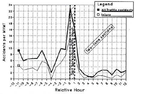
- ii -

List of Tables

Table 3-1: Summary of Study Sites ................................. 13
Table 4-1: Descriptive Statistics of the Data ............................ 22
Table 4-2: Summary Results of GNB and PLN Models for combined dataset ...... 25
Table 5-1: Elasticities of Main Influencing Factors ....................... 29
Table 6-1: Comparison of the Two Studies ............................ 41
Table 6-2: Collision Rates Before and After Maintenance Operations and Percent
Reduction .................................................. 43

List of Figures

Figure 2-1: Traffic Collision Rates Before and After Salt Spreading (Source: Salt
Institute) .................................................... 5
Figure 3-1: Methodology ........................................ 10
Figure 3-2: Relation between Weather, Traffic Maintenance, and Safety ......... 12
Figure 3-3: Ontario Road Network and Study Sites (thick lines) ............... 13
Figure 3-4: Road Surface Conditions over a Snow Storm Event ............... 20
Figure 5-1: Effect of Different Factors on Relative Risk .................... 33
Figure 5-2: Safety Effect of Salting ................................. 35
Figure 5-3: Safety Effect of Plow & Salting (Operation Done at Hour 2) ......... 37
Figure 5-4: Safety Benefit vs. Maintenance Timing ....................... 37
Figure 5-5: Safety Benefit of Salting ................................. 39
Figure 6-1: Illustration of Factors That May Confound the Effect of Salting ....... 44
Figure 6-2: Collision Rates Before and After Maintenance Operations .......... 42
- iii -
Executive Summary
Significant research efforts have been devoted to quantifying the safety and mobility
impacts of winter weather and developing cost-effective snow and ice control strategies
and methods. However, most of these efforts have not reached to the level of
understanding that is required to support decision-making at both operational and
strategic levels. The goal of this research is to conduct a systematic investigation aimed at
addressing this knowledge gap.
This report summarizes the results of an analysis performed on a set of collision data over
six winter seasons (2000-2006) from 31 sections of highways in the province of Ontario.
Several statistical models were developed to evaluate the association between road safety
and winter road maintenance treatments and other factors. The main findings from the
models and case studies are summarized as follows.
Factors Affecting Winter Road Safety
Most results obtained from this research with respect to winter road safety are
consistent with those reported in the literature, with a few exceptions. The severer the
storm conditions are, as indicated by temperature, visibility, wind speed and
precipitation, the higher is the expected number of collisions.
The most interesting result is that the road surface condition index (RSI) was found to
be a statistically significant factor influencing road safety across all sites, models and
functional forms. It is the most influential risk factor with a 10% improvement in road
surface conditions could lead to 20% reduction in mean number of collisions. RSI is a
surrogate measure of road surface conditions and can thus be used to capture the
effects of winter road maintenance operations, making it feasible to quantify the
safety benefit of alternative maintenance policies and methods.
Visibility and precipitation were found to be the next most prominent factors
influencing road safety under adverse weather conditions. A 10% reduction in
visibility or increase in precipitation rate could result in almost 5% and 0.2% increase
in the mean number of collisions, respectively. Wind speed and temperature were
also found to be statistically significant collision risk factors; however, the magnitude
of their effects was much less as compared to other factors.- iv -
Benefits of Salting
The collision models developed in this research provide a new way of quantifying the
safety effect of winter road maintenance operations such as salting and plowing. By
controlling for the external factors such as weather, road geometry and traffic, their
potential confounding effects on the benefit estimates could be minimized. The
modeling results has provided clear evidence on the safety benefit of salt application,
reducing collisions from 20% to as high as over 85%, depending on the base
conditions when salt is applied and the improved conditions due to the deicing effect
of salt.
Two case studies were conducted to illustrate the application of the developed models
for evaluating the safety benefit of maintenance operations at an operational level
involving a particular section of highway and snowstorm event. It is also shown that,
instead of relative reduction, the absolute benefit could also be determined using the
developed models, which is a function of the type of highway being considered (e.g.,
traffic volume) as well as other weather variables such as precipitation, visibility,
wind speed and temperature.
An analysis similar to the Marquette study was also performed using the Ontario data.
Two different types of events were extracted from the main database– events where
either salting was the sole operation or events where salting was applied in
conjunction with plowing. The former allows us to gauge the sole effects of salting
operations on winter road safety. An overall reduction of 51% was observed in the
collision rate before and after salt application while a total of 65% reduction was
associated with the combo operations of plowing and salting. While these benefit
estimates are lower than those obtained by the Marquette study (which showed over
78% reduction in collisions on freeways and 87% reduction on two-lane highways),
this analysis has nevertheless confirmed the overall findings of the Marquette study.-1- 1. INTRODUCTION Winter storms have a significant impact on the safety and mobility of highways. Past research indicates that highway collision rates during a snowstorm increase considerably as compared to a non-winter storm season (Andrey and Knapper 2003). Slippery road conditions and poor visibility during a winter storm also create unbearable travel environments for travelers and cause substantial delay due to reduced traffic speed and road capability and increased collisions. To reduce the impacts of winter storms, transportation agencies spend significant resources every year to keep roads and highways clear of snow and ice for safe and smooth travel conditions. For example, Canada expends $1 billion each year on winter road maintenance, which includes the application of five million tons of salts (Transport Association of Canada, 2003). In the US, the total cost of winter road maintenance is approximately $2 billion per year. Salt use has recently raised significant concerns due to their potential damages to the environment, the road side infrastructure, and the vehicles. While it is commonly agreed that winter road maintenance (salt) is beneficial to both safety and mobility of highways, it is however unclear about the magnitude of this benefit and the factors that influence this benefit. This knowledge gap makes it difficult to address the question of what should be the optimal amount of maintenance work (or salt) being applied for a given highway or jurisdiction under particular winter conditions. Many attempts have been made in the past to address this knowledge gap. Most of those studies have however focused on the general impacts of winter storms on road safety and mobility. For example, Knapp et al. (2000) investigated the effects of winter storms on mobility and safety using data from a freeway section in Iowa. Their study found that the average collision rate increased by several orders of magnitude during storm events and the degree of impacts depended on storm duration, snowfall intensity and wind speed. Recently, Andrey and Knapper (2003) investigated the effects of weather on the transportation system at a national level. Note that these studies did not look into the particular issue of how winter road maintenance work affects road safety and therefore may underestimate the true effect of winter storms. As synthesized by Wallman et al. (1997), most past studies on the effect of winter road
-2-

maintenance have shown significant benefits in reducing collision rate and severity. For
example, an extensive study in Germany (Hanke and Levin, 1989) showed the average
collision rate dropped by 73% within two hours of salt applications. Hanbali and
Kuemmel (1993) conducted a similar analysis on traffic crash rates before and after salt
application on two types of highway, namely, two-lane two-way highways and freeways
in several US states. They found an average of 85% reduction in traffic crashes and an
88.3% reduction in injury-causing collisions just within a few short hours of applying
salt. Similar findings were observed in several Swedish and Nordic investigations
(Wallman et al. 1997).

A scientific approach to achieving optimal balance of keeping road safe and
environmental effect minimal requires a better understanding of the relationship between
highway performance, such as collision rates and traffic delay, and maintenance
operations under a variety of storm and road surface conditions. The primary goal of this
research is to quantify the safety benefit of winter road maintenance operations such as
salting in the Canadian environment with field data from Ontario, Canada. To ensure the
validity of the results, the research will attempt to account for other confounding factors
such as storm characteristics (e.g., temperature, precipitation, and wind speed) and road
and traffic characteristics (e.g. classification, speed, volume), in addition to maintenance
operations. The research includes the following three main objectives:

   1) Conduct a thorough and critical review of past studies on the effects of winter
      road maintenance on road safety;
   2) Investigate the collision frequency and severity patterns before and after various
      specific maintenance operations, such as plowing and salting, during individual
      winter snow storms;
   3) Develop statistical models for quantifying the safety benefit of winter road
      maintenance and identifying the major factors that influence this benefit;
-3- 2. LITERATURE REVIEW Significant past efforts have been directed towards road safety problems in general and winter road safety in particular. This section provides a review of studies that focused specifically on the effect of winter road maintenance on road safety. For other general winter road safety issues and research, readers are referred to Andrey et al. (2001), Shankar et al. (1995), Hermans et al. (2006), Nixon and Qiu (2008), and Qin et al. (2007) etc. Weather has both direct and indirect impacts on highway safety. According to Ontario Road Safety Annual Report (MTO, 2002), in spite of the rare occurrence of adverse weather in daily traffic, many crashes occurred during rainfall and snowfall in Ontario (11.4 percent and 10.6 percent of total crashes, respectively). Also, crashes that occurred on wet and snowy road surface account for high proportions of total crashes (19.0 percent and 14.1 percent, respectively). This is because adverse weather reduces the friction between vehicles and the road surface and visibility, and drivers are more likely to misjudge prevailing friction conditions (Wallman et al, 1997). A similar trend was observed in the United States where over 22 percent of total crashes were weather- related, of which 49 percent and 13 percent occurred during rainfall and snowfall respectively (Goodwin, 2002). Nilsson and Obrenovic (1998) found that drivers are twice as much likely to be involved in a collision in winter than in summer for the given distance of travel. Wallman et al. (1997) observed that more crashes tend to occur at the beginning of a winter season and when there are fewer snowy road conditions. However, some past studies have also concluded that snowfall-related crashes tend to be less severe than those under other weather conditions (Andrey et al., 2003). One possible explanation provided for this finding is that vehicles tend to travel slower under snow storm conditions than normal weather conditions (Knapp et al., 2000). A study by Iowa State University (Knapp and Smithson, 2000) focuses on the effects of winter storms on traffic safety for a 48-km long highway section in Iowa. They concluded that crashes are more likely to occur during storm event time periods (2 crashes/event) than non-storm event time periods (0.65 crashes/event). However, this study limited the scope of winter storms to those storm events with more than 4-hour
-4-

duration and more than 0.51 cm/hour snowfall intensity. Also, their analysis did not
consider whether or not winter maintenance activities had been performed during or after
storm events.

Khattak et al. (2000) found that there is a close relationship between crash frequency and
characteristics of storm events such as snowfall intensity, snow fall duration, and
maximum wind gust speed. They also considered the effect of exposure (i.e. number of
vehicles during a snowfall event on a highway section under the same weather condition)
and found that a snowfall event reduces traffic volume (i.e. exposure to hazardous road
conditions) which results in a higher crash rate.

Note that these studies had mainly focused on the effects of the characteristics of storm
events on crash risk and the effects of “controllable” variables such as maintenance
operations on preventing or reducing crashes during winter storm events were not
considered.

There are abundant empirical evidences showing that winter road maintenance
significantly improves road safety. Quantitative investigations on this subject were
however scarce. One of the first documented studies in the literature on the effect of
winter road maintenance on road safety was performed by the Technical University of
Darmstadt in Germany (Hanke and Levin, 1989). The study involved a statistical analysis
of collisions before and after salt applications on 650 kilometres of roads in suburban and
rural areas. The main finding of this research is reflected in the well cited illustration
shown in Figure 2-1.

Hanbali and Kuemmel (1992) from Marquette University conducted a similar study
applying the same methodology as the German study (Hanke and Levin, 1989) using
collision data from 570 miles of divided and undivided roads from New York,
Minnesota, and Wisconsin. Their analysis corroborated the German study and concluded
that significant reductions in collisions were observed after salting operations. The
average reduction in collision rates was 87% and 78% for two-lane undivided highways
and freeways, respectively. It should be noted that the before-after analysis approach
taken by these two studies did not take into account the confounding effects of many
important factors, such as precipitation, temperature, and visibility, which vary over
events and before and after salt applications. As a result, they may over or under estimate
the benefit of winter maintenance operations (including salting), which is expected to
vary by external conditions such as highway features, storm characteristics and
maintenance treatments.
-5-

                                 (a) German Study

                         (b) Marquette University Study
Figure 2-1: Traffic Collision Rates Before and After Salt Spreading (Source: Salt
                                     Institute)
-6- Norrman et al. (2000) conducted a more elaborated study to quantify the relationship between road safety and road surface conditions. In their study, they classified road surface conditions into ten different types based on slipperiness, and then compared the crash rates associated with the different road surface types. They defined collision risk for a specific road surface condition type, as the ratio of the collision rate under a road surface condition to the expected number of collisions. The collision risk computed was then compared to the percentage of maintenance activities performed. They concluded that, in general, increased maintenance was associated with decreased number of collisions. However, their approach has several limitations. Firstly, it is an aggregate analysis in nature, considering roads of all classes and locations together. This approach may mask some important factors that affect road safety, such as road class and geometrical features, traffic, and local weather conditions. Secondly, the simple categorical method of determining crash rates may introduce significant biases if confounding factors exist, which is likely to be the case for a system as complex as highway traffic. Furthermore, the procedure cannot be used to quantify the safety effects of different maintenance operations. Fu et al. (2006) investigated the relationship between road safety and various weather and maintenance factors, including air temperature, total precipitation, and type and amount of maintenance operations. Two sections of Highway 401 were considered. They used the generalized linear regression model (Poisson distribution) to analyze the effects of different factors on safety. They concluded that anti-icing, pre-wet salting with plowing and sanding have statistically significant effects on reducing the number of collisions. Both temperature and precipitation were found to have a significant effect on the number of crashes. Their study also presents several limitations. First, the data used in their study were aggregated on a daily basis, assuming uniform road weather conditions over entire day for each day (record). Secondly, their study did not account for some important factors due to data problems, such as traffic exposure and road surface conditions. Furthermore, the data available for their analysis covered only nine winter months and thus the power of the resulting model needs to be further validated. One of the implications of these limitations is that their results may not be directly applicable for quantifying the safety benefit of winter road maintenance of other highways or maintenance routes. The Swedish Road and Traffic Road Institute (VTI) had investigated the relationship between winter road safety and road maintenance for many years with most of the findings summarized in a reviewing report completed by Wallman et al. (1997). Many original research reports cited by Wallman et al. (1997) were written in Swedish and could not be included for a detailed discussion in this literature review. The following
-7-
summarizes the findings from several major studies documented by Wallman et al.
(1997):
The collision rate reached its maximum one hour before the maintenance action
and the collision rate was reduced by 50 percent a half-hour after the action. The
number of collisions was reduced to 1/6 6-12 hours after winter maintenance was
implemented. They also cited that the numbers of collisions were reduced to
1/5~1/14 and 1/8 after maintenance was carried out in Germany and U.S.,
respectively. These findings demonstrate that winter road maintenance does
improve road conditions and lower crash risk.
Some before-after studies and parallel comparisons of similar roads with different
maintenance intensities indicated that the effects of road salt with regard to road
safety could not be statistically confirmed. It had been reported that reduction in
crash frequency was not in proportion to the improvement in road conditions.
Many studies attributed these counter-intuitive results to the road user’s risk
compensation behavior, that is, road users utilize the increase in road friction (e.g.
due to salting) by increasing their speed.
It has been observed that preventive salting (anti-icing) was more effective in
reducing the crash rate than conventional salting.
In summary, a number of past studies have been dedicated to the issue of winter road
safety. However, most of these studies have focused either on the effect of weather only
or suffered some methodological issues, with the following specific limitations:
Most research relied on data that were either incomplete or aggregated. For
example, many studies have used aggregated seasonal and yearly average for
weather and traffic conditions because daily and hourly weather and traffic counts
were not available. Also, road condition data and collision reports obtained from
different organizations were not consistent with each other.
Most investigations cover large regions with large spatial (e.g. cities, provinces)
and temporal (e.g. daily, seasonal, annual) analysis units. Such macro-level
analysis cannot take into account local variations in weather and road conditions,
traffic and maintenance operations.
Very little empirical evidence exists in literature regarding the effects of winter
road maintenance treatments on road safety, mostly, due to the fact that detailed
maintenance records were not available.
Most findings and results reported in literature were obtained directly from
observations with naive before-after analysis with few resulting from systematic
statistical analysis.-8- To cope with these problems, this research proposed a disaggregate methodology to investigate the relationship between winter road safety and winter road maintenance activities. Patrol route (road section maintained by a single contractor for maintenance purpose) is used as the spatial level of analysis and snow storm event or hourly observations (within the snow storm event) as the temporal unit of analysis. The following section provides a detailed description of the methodology adopted and the data used.
-9-

3.          METHODOLOGY AND DATA

3.1 OVERVIEW OF METHODOLOGY

A statistical modeling approach is proposed to investigate the relationship between winter
road safety and various influencing factors, including maintenance operations (e.g.,
salting). Figure 3-1 shows the steps being followed in the development of these statistical
models, including:

   1) Selection of Study Sites: this is done on the basis of the availability of weather &
      road surface, traffic and collision data.
   2) Data Processing and Integration: data from the different sources are compiled and
      subsequently integrated into a single cross-sectional, hourly-based dataset using
      location and time as the references.
   3) Exploratory Data Analysis and Model Development: an exploratory data analysis
      is first performed for understanding the data and identifying the qualitative
      patterns. Statistical models are then developed for quantitative relationship
      between the road safety indicators (e.g., expected collision frequency) and various
      external factors.
   4) Model Application: the developed models are lastly applied for assessing the
      effects of salting or generally winter road maintenance operations on road safety.

A detailed discuss on these individual steps is provided in the following sections.
- 10 -
SELECT STUDY SITES (HIGHWAY ROUTES)
Traffic Weather and Collision
Volume Road Surface Data
Data Data
DATA INTEGRATION
Hourly Based Data
Exploratory Data Analysis
Generalized Linear Models Generalized Linear Models
(PLN, GNB) (NB, GNB)
Findings and Applications
Figure 3-1: Methodology
3.2 STATISTICAL MODELS
In road safety literature, the most commonly employed approach for quantifying the
effects of different factors on road safety is the generalized linear regression analysis.
Specifically, the negative binomial (NB) model and its extensions have been widely used
for modeling road collisions (Hauer 1997; Miranda-Moreno 2006). In this research, we
have adopted the same modeling approach. Specifically, two alternative models are
considered, including multilevel Poisson lognormal model (PLN) and generalized
negative binomial (GNB) model (Miaou and Lord 2003; Miranda-Moreno et al 2005;
Miranda-Moreno 2006). These models allow more flexibility than the basic NB model in
dealing with the well-known over-dispersion problem and unobserved heterogeneities in
collision data.- 11 -
The PLN model differs from NB model in the sense that a lognormal distributed error
term (instead of gamma distribution) is added to the Poisson model to capture the
unobserved heterogeneity. This model also has the advantage that can be easily extended
to deal with data of multi-level nature, which is the case with the data we have. As
detailed in the following section, the hourly collision data over individual snow storms is
longitudinal in nature with the hourly records within each storm forming a set of repeated
measurements over time, and the number of time periods being constant for each
observation site (route). The potential within-storm correlation issue can be addressed by
this model structure (Usman et al 2012; Miranda-Moreno 2006; Miranda-Moreno and Fu
2006). Moreover, the lognormal tails are known to be asymptotically heavier than those
of the Gamma distribution (Kim et al 2002). This can be the case when working with
dataset in the presence of outliers (Winkelmann 2003).
In a multilevel setting, a PLN model for the hourly observations at the event level can be
represented by Equation 3 – 1 and 3 – 2.
Yim ~ Poisson (im), with ln(im) = im + m + im (3 – 1)
Where, im and im are defined as the number and mean number of collisions in hour i
belonging or nested in the storm m. In addition, m is a patrol route-level random effect,
following a Normal distribution, i.e., m ~ N(0, 2) and im is the model error - also normal
distributed, im ~ N(0, ). Note that im represents all the unobserved heterogeneities or
random variations that are not captured by m; while, m represents event-level
unobserved factors controlling for the potential within-event correlation. In this case, the
equation for the mean collision frequency has the following functional form:
im ( Exposurem ) exp( 0 2 xi1m 3 xi 2m k xikm )
1
(3 – 2)
These models are then calibrated using the data set in the following section.
3.2 DATA SOURCES AND DATA INTEGRATION
There are a large number of factors that influence the safety of a highway under winter
conditions (Andrew and Bared 1998; Miaou et al 2003). The major factors affecting
winter road safety can be grouped into three categories, namely, weather characteristics,
traffic, and maintenance operations, as schematically illustrated in Figure 3-2 (Usman et
al 2010).- 12 -
Figure 3-2: Relation between Weather, Traffic Maintenance, and Safety
Models can be developed by establishing a relationship between collision frequency and
these factors. Analyses could be performed at an aggregate level, e.g., event-based
analysis (Usman et al 2010) or at disaggregate level, e.g., hourly-based analysis (Usman
et al 2012). This report describes the latter approach with the following five steps:
Selection of study sites
Data source identification (traffic, weather, maintenance and collision data)
Data processing (hourly data and storm-event data)
Modeling road surface conditions
Exploratory data analysis and development of statistical models
Study Sites
MTO has divided the province of Ontario into five different regions, namely, Central
(CR), Eastern (ER), South-West (SWR), North-West (NWR) and North-East (NER).
These regions are further subdivided into different contract areas. Each contract area
contains multiple patrols and each patrol covers different routes. A route covered by a
patrol for a particular highway is known as “patrol route” for that highway. Spatially,
highway sections designated by these patrol routes are selected as the basic analysis units.
To fulfil the purpose of this research a temporal aggregation level of one hour is- 13 -
considered as the minimum analysis unit. It was found that detailed hourly traffic data is
not available for all the sites/patrol routes. Accordingly sites were selected where such
data was available. Based on traffic data availability, a set of 34 sites were selected which
were further reduced to 31 due to data unavailability from other data sources. Details of
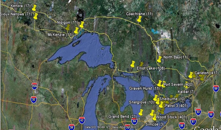
the selected sites are given in Table 3-1 and Figure 3-3.
Table 3-1: Summary of Study Sites
Highway Class No. of Sites (Routes) Total Length AADT Range
Freeway 17 753.6 14,600 to 430,000
4-lane Highway 3 127.71 5,000 to 129,000
2-lane Highway 11 874.1 400 to 17,700
31 Highway routes
1,755 Km
2000-2006 Winter
seasons
58 Events/site/season
122,000 Event hours
Figure 3-3: Ontario Road Network and Study Sites
After the sites were finalized, data collection was started. The time span selected for data
collection was set to the period October 1999 to April 2010. However, due to
unavailability of data from some sources, the final analysis period was restricted to the
time frame of October 2000 to April 2006 (six winter seasons). Hourly data was obtained
from each data source (details in the following section) for each site.- 14 -
Data Sources
Five types of data were obtained and compiled, including weather data, traffic data,
collision data, road surface condition data and winter operations data. These data were
gathered from different sources and managed by different organizations. This section
provides a description of these data sources.
Traffic Volume Data
Traffic volume data for each study site is obtained from two sources. The first source is
traffic data from MTO’s permanent data count stations (PDCS). PDCS provided traffic
counts in different resolutions, including 15 minutes, 30 minutes, hourly and daily. Some
of the stations also contained speed information.
The second data source is from loop detectors. This data is collected at 20 seconds
interval and contains information about speed, traffic flow and density. This data was
provided in an hourly format by MTO for this research. The original data is organised by
individual loop detectors. These loop detectors are located on Highway 400, 401, 404,
410 and QEW. Loops belonging to a particular patrol route on the highways mentioned
were identified and processed together. Both data sources were screened for any outliers
caused by detector malfunction.
Traffic Collision Data
The Ontario Provincial Police (OPP) maintains a database of all collisions that have
occurred on Ontario highways. This is “person based” data and includes information
related to individuals as well as vehicles involved in each collision. A total of 147
variables are recorded. A database including all collision records for the study routes was
obtained from MTO for the ten winter seasons (1999-2009).
The database includes detailed information on each collision, including:
Collision time
Collision Location
Collision type
Impact type
Severity level- 15 -
Vehicle information
Driver information
Road conditions – surface and geometry
Weather conditions
Speed
Visibility
Note that the data on the collision occurrence time and location are needed for data
aggregation over space (e.g., highway maintenance route) and time (e.g., by hour). The
data items related to weather and road surface conditions represent only the conditions at
the time and location associated with the observed collisions and therefore do not
necessary represent the whole maintenance route. As a result, we did not use this data
field directly and instead used it to complete any missing RSC data which was primarily
sourced from MTO’s road condition weather information system (RCWIS) and road
weather information system (RWIS).
Road Condition Weather Information System (RCWIS) Data
This data contains information about road surface conditions, maintenance, precipitation
type, accumulation, visibility and temperature. RCWIS data is collected by MTO
maintenance personnel, who patrol the maintenance routes during storm events; 3 to 4
times on the average. Information from all patrol routes are conveyed to a central system
six times a day. Instead of stations this data is collected for road sections. Each
observation contains information regarding the section of road to which it belongs. One
of the most important pieces of information in this data source is description of road
surface condition, which is used in this study as a primary factor for collision modeling.
A detailed description on this data field and its processing for the subsequent modeling
analysis is given in later sections. This data is also used by MTO in their traveler’s road
information system; however, this is the first time that it has been utilized for research
purposes.
Road Weather Information System (RWIS) Data
This data source contains information about temperature, precipitation type, visibility,
wind speed, road surface conditions, etc., recorded by the RWIS stations near the selected
maintenance routes. All data except precipitation were available on an hourly basis.
Hourly precipitations from RWIS sensors were either not available or not reliable. As a
result, we derive this information from the daily precipitation reported by Environment- 16 - Canada (EC). Temperature and RSC data from RWIS were used to fill in the missing data from RCWIS. For visibility and wind speed RWIS was used as the primary source. RWIS stations record data every 20 minutes. Environment Canada (EC) data Weather data from Environment Canada (EC) includes temperature, precipitation type and intensity, visibility and wind speed. Except precipitation related information, all data from this data source are used as a secondary source for filling in the missing data from RCWIS/RWIS. EC is the only reliable data source for precipitation type and intensity and it is therefore used as the primary source for these variables. Data is available at different time resolutions; but hourly data was selected for the purpose of this research. Data Processing As described previously, there are three main types of data available for each selected study site. Once these data were obtained, they were pre-processed for subsequent merging and integration. Details on the steps involved are described in the following sections: Traffic volume data: the traffic volume data is obtained from two sources: permanent data count stations (PDCS) sites, and loop detectors. Data from both sources is in hourly format; however, some pre-processing is required. These sources are used to supplement each other when data from one of the data source is missing. In cases where data is available from multiple loop detectors and/or PDCS sites, an average is used. Collision data: collision data is compiled as person/occupant based data (Note that person and occupant are used interchangeably in this research). Each observation in the data belongs to an individual person involved in a collision. A stepwise aggregation approach is used to compile this data into hourly records by totalling the collisions that occurred within each hour of the day. Other attributes associated with collisions are averaged for each hour. In the collision data (occupant based) each person and vehicle involved in a collision are identified uniquely. This dataset is first converted to vehicle-based data, then to collision based data, and finally to hourly based data. Weather and road surface data: weather data are obtained from three different sources: RCWIS, RWIS and EC. Most of the weather data from MTO’s RCWIS is descriptive (or categorical) in nature. The data is thus coded to fulfill the specific purpose of this research. RCWIS data, organized by patrol route, is descriptive in nature, similar to
- 17 -

event-based records with a time stamp. As a result, two immediate issues needed to be
addressed. First, the original RCWIS data classifies road surface condition into seven
major classes with a total of 486 sub-classes, making it difficult to use it as a categorical
factor in a statistical analysis. Secondly there was missing information - a large number
of hours did not have RCWIS observations. These issues were addressed by converting
RSC to a scalar variable. This is discussed in detail in the following section. RCWIS data
is converted to hourly data whenever the observations are available by taking the average
of the variables within that hour and counting the number of different WRM operations
performed within that hour. RWIS data is recorded every 20 minutes and is converted to
hourly data by averaging observations within an hour. In cases that more than one RWIS
stations are available for a single site, their average value is used. Data from Environment
Canada is available in five different formats:

       1)   Data prefixed by MIN is hourly record of data recorded each minute
       2)   Data prefixed by FIF is fifteen minute data
       3)   Data prefixed by HLY is daily record of hourly data
       4)   Data prefixed by DLY is monthly record of daily data
       5)   Data prefixed by MLY is annual record of monthly data

Hourly format is chosen as it suites our data needs. However, precipitation data is mostly
available in the daily data-format, which is the water equivalent of the total precipitation
amount over a day. Data was downloaded from Environment Canada website1 for 389
stations. 217 Stations were selected based on their proximity to the sites. Out of these 217
stations were used in this research - 69 stations with hourly data and 171 stations with
daily data (Precipitation data). These stations are selected using a two-step process. First,
an arbitrary 60 Km buffer is assumed around each site and sites falling within that
boundary are selected. In the next and final step, stations closer to patrol routes are
selected as control stations. Each control station is compared with other stations lying
close to the control station using a paired t-test to determine whether stations distant from
the control stations have a statistically different mean for each variable compared to the
control stations. This step is necessary to select only stations with weather conditions
similar to the control stations, which in turn represent the conditions at the patrol route.
If, for a station, a variable, e.g., visibility is showing a significant difference in its mean
from the mean visibility value of the control EC station near patrol route, the variable is
removed. In the case that all variables show a significant difference, the whole station is
discarded. Data from multiple stations are used to ensure that there are no missing values

1
    http://www.climate.weatheroffice.gc.ca/climateData/canada_e.html
- 18 - and to capture the average effects for a patrol route. Arithmetic mean is found to give better results than weighted average. Precipitation intensity data is available only as a daily total, which is the water equivalent of the total precipitation amount over a day. Based on the data describing “precipitation type” the hours with and without snow/freezing rain precipitation are identified. The total precipitation amount of each day is then uniformly allocated to the individual hours of the day during which precipitation occurred. Once all the data’s are converted into an hourly format, they are then fused into a single dataset on the basis of date (day), time (hour) and location (patrol route). Some of the variables in this dataset are duplicated as these variables are present in different data sources. In these cases priority is given to RCWIS data then RWIS data and then EC data because the former data sources are collected nearer the study sites and are therefore considered to be more representative. Similarly in case of any missing data for temperature, precipitation or wind in RCWIS, data from RWIS or EC data is used. Missing RSC data from RCWIS are retrieved from collision data or RWIS data. It is also assumed that the RSC for the hour directly following maintenance activities could be considered as at least partially snow covered. This data field is then subsequently linearly interpolated for hourly conditions, as discussed in the following section. This gives us values for road surface condition for all hours over individual storms. Once the three sources of data are finalized, a single dataset is formed by combining all datasets on the basis of date (day), time (hour) and location (patrol route). This process resulted in an hourly-based dataset. Modeling of Road Surface Conditions MTO reports RSC using qualitative descriptions, i.e., a categorical measure (with 7 major categories and 486 subcategories). These categories have intrinsic ordering in terms of severity, which means that a more sensible measure would be an ordinal one. While binary variables could be used to code ordinal data, it would mean loss of information on the ordering. We therefore decided to use an interval variable to map the RSC categories and at the same time make sure that the new variable would have physical interpretations. Road surface condition index (RSI), a surrogate measure of the commonly used friction level, was therefore introduced to represent different RSC classes described in RCWIS. The reason that we used a friction surrogate is that there have been a number of field studies available on the relationship between descriptive road surface conditions and friction, which provided the basis for us to determine boundary friction values for each category. To map the categorical RSC into RSI, the following procedure was used
- 19 -

(Usman et al 2010):

   1. The major classes of road surface conditions, defined in RCWIS, were first
      arranged according to their severity in an ascending order as follows:
      Bare and Dry < Bare and Wet < Slushy < Partly snow covered < Snow
      Covered < Snow Packed < Icy. This order was also followed when sorting
      individual sub categories in a major class.

   2. Road surface condition index (RSI) was defined for each major class of road
      surface state defined in the previous step as a range of values based on the
      literature in road surface condition discrimination using friction measurements
      (Wallman et al 1997; Wallman and Astrom 2001; Transportation Association of
      Canada 2008; Feng et al 2010). For convenience of interpretation, RSI is assumed
      to be similar to road surface friction values and thus varies from 0.05 (poorest,
      e.g., ice covered) to 1.0 (best, e.g., bare and dry).

   3. Each category in the major classes is assigned a specific RSI value. For this
      purpose, sub categories in each major category were sorted as per step 1 above.
      Linear interpolation was used to assign RSI values to the sub categories.

   RSI values for major road surface classes are given below:

       Road Surface Condition major Classes          RSI Range
       Bare and dry                                  0.9~1.0
       Bare and wet                                  0.8 ~ 0.9
       Slushy                                        0.7 ~ 0.8
       Partly snow covered                           0.5 ~ 0.7
       Snow covered                                  0.30 ~ 0.5
       Snow packed                                   0.2 ~ 0.3
       Icy                                           0.05 ~ 0.2

Database Integration and Pre-processing

The data obtained from all the data sources were subsequently pre-processed and merged
to form a data set of hourly records on weather, traffic, and collisions. Snow storm events
are then identified based on weather conditions and road surface conditions, as shown in
Figure 3-4. The following assumptions were considered in the event identification
process:
- 20 -
Each event is defined with the following constraints:
An event starts at the time when snow/freezing rain is observed;
An event ends when snow/freezing rain stops and a certain predefined road
surface condition is achieved after that time.
Precipitation must be greater than zero (0 cm/hr)
Air temperature must be less than 5 oC
Road surface conditions index value must not be equal to bare dry conditions
Maintenance
Operation
Storm
Bare Pavement (BP) Status
Starts Predefined BP
Storm Ends Target Regained
1
EVENT DURATION
Incident
0
** * Time
Figure 3-4: Road Surface Conditions over a Snow Storm Event
A total of 10932 route-events are extracted based on the event definition and restriction
defined above. A total of 3035 collisions were observed over these events.- 21 -
4. DATA ANALYSIS AND MODEL
CALIBRATION
4.1 EXPLORATORY DATA ANALYSIS
A total of 32 datasets (31 individual sites and one combined set) were formed for the 31
sites selected. Inconsistencies were verified through exploratory analysis. Descriptive
statistics were computed. The combined data set has a total of 122,059 observations
recorded over 10,932 snow events. All the data sets were checked for any outliers using
box plots of individual data fields in the database.
For the purpose of the subsequent modeling analysis, the following variables were
defined:
Total number of collisions over an hour (Y, dependent variable)
Indicator for month (M, including October, November, December, January,
February, March, and April)
Indicator for hour of the event (FH, FH = 1 if first or second hour, 0 otherwise)
Average air temperature (T, Co)
Average wind speed (WS, km/hr)
Average visibility (V, km)
Precipitation intensity - hourly precipitation (HP, cm)
Average road surface index (RSI)
Precipitation type (PT, PT = 1 for freezing rain/ snow; 0 otherwise)
Indicator for winter road maintenance operation type (WRM, including sanding,
salting, ploughing, and a combination of them)
Exposure defined as the product of segment length and hourly traffic, in million
vehicle kilometres traveled (EXP, MVKm)
Site indicator (S, including all 31 sites)
Month was included as a variable to test monthly trend over a season. To test the trend
within a storm, time factors were included in the analysis to check whether the start of the- 22 -
event is more susceptible to collisions compared to the rest of the storm. It was found
that the effect of the first hour against other hours in the snow storm (FH) was significant.
Site-specific effects were included in the models to take into account the potential effects
of specific unmeasured factors on road safety, such as driver population, and road
geometry.
For this purpose, three different fixed effects were investigated:
Site-specific fixed effects using a dummy variable for each site
Region-specific effects using a dummy variable for each region
Road-type specific effects using a dummy variable for each road type
Ontario province is divided into 5 regions given below:
Region 1 - Central Region
Region 2 - Eastern Region
Region 3 - North-Eastern Region
Region 4 - North-West Region
Region 5 - South-Western Region
A correlation analysis was conducted for each patrol dataset and the combined dataset. It
was found that precipitation type and maintenance operations were consistently
correlated with RSC across all datasets (with a correlation coefficient greater than 0.60)
and were therefore removed from further analysis. Descriptive statistics are given in
Table 4-1.
Table 4-1: Descriptive Statistics of the Data
Wind Hourly Event
No. of Temp Visibility Ln
Speed Ppt RSI Duration
Collisions (co ) (km) Exp
(km/hr) (cm) (hr)
Sample Size (N) = 122,058
Min 0 -33 0 0 0 0.05 2 3.8
Max 7 28 69 40 13.8 1 47 14.3
Mean 0.02 -5 16 11 0.24 0.75 19 8.0
St.
Dev 0.18 6 10 8 0.37 0.20 11.6 1.7- 23 -
4.2 MODEL CALIBRATION
After identifying the modeling approach, the next step was to fit the models to the data.
Though models were calibrated for all the 32 data sets, only the combined data will be
discussed here because of the relatively large sample size which makes it feasible to
check the effects of different site specific factors. Results obtained with larger samples
are more trustworthy (Wright 1995).
The data used in this research is a 2-level hierarchical dataset where storm hours are
nested within individual storms. This type of data generally suffers from within subject
correlation. Intra-class correlation (ICC) (correlation among observations within the same
storm event) was computed for this correlation. ICC, denoted by , has a value ranging
from 0 to 1. This means that if all hourly collision count observations are independent of
one another, then = 0. On the other hand, if observations inside each cluster (in this
case, storm) are exactly the same, = 1 (Usman et al. 2012). Obviously, a 0 implies
that the observations are not independent, e.g., ICC > 0 implies that the collision
occurrence in the same storm is influenced by similar unobserved storm factors. ICC for
this dataset comes out to be 6.05%. Though there is no set rule for the ICC value; a value
close to zero suggests the presence of weak correlation. Under such circumstances the
less complex single level models could also be applied to this data. In such cases the
distortion effect of the correlation on the parameter estimate is expected to be minimal.
The following models were calibrated:
A. Poisson lognormal - Two Level Models
PLN1: A model without any spatial factors
PLN 2: A model with regional effects
PLN 3: A model with road type effects
PLN 4: A model with site effects
B. Generalised Negative Binomial - Single Level Models
GNB1: A model without any spatial factors
GNB2: A model with regional effects
GNB3: A model with road type effects
GNB4: A model with site effects
Site-specific variables are included in the specification of each model to capture the
possible effect of other route specific factors (such as location, driver population, and- 24 -
road geometry, on road safety). All models were calibrated using Stata2 (Version 11). A
stepwise elimination process was followed to identify the significant factors. The best fit
model was identified using likelihood ratio test and Akaike Information Criterion (AIC)
(Akaike 1974). The AIC statistic is defined as -2LL+2p, where LL is the log likelihood of
a fitted model and p is the number of parameters, which is included to penalize models
with higher number of parameters: a model with smaller AIC value represents a better
overall fit. Based on both the likelihood ratio test and AIC criterion, the GNB4 model
calibrated, considering the effects of the first hour of a storm and site specific variables
was found to be the best fitted model for the combined data set. Table 4-2 shows the
modeling results for GNB and PLN. The GNB model is given in Equation 4-1.
(4-1)
where µ = Mean number of collisions
T = Temperature (C)
WS = Wind Speed (km/hr)
V = Visibility (km)
TP = Total Precipitation (cm)
HP = Hourly Precipitation (cm)
RSI = Road surface index representing road surface conditions
EXP = Exposure (total traffic in an hour multiplied by length of the section,
MVKm)
M = Indicator for month (Table 4-2)
S = Indicator for site (Table 4-2)
FH = Dummy variable for the effect of first hour (-0.302 if first hour, 0
otherwise).
These modelling results are used for identifying the factors that have a significant effect
on winter road safety and the magnitude of these effects, as discussed in the following
section.
2
http://www.stata.com/- 25 -
Table 4-2: Summary Results of GNB and PLN Models for combined dataset
GNB1 PLN1 GNB2 PLN2 GNB3 PLN3 GNB4 PLN4
Variable
B Sig B Sig B Sig B Sig B Sig B Sig B Sig B Sig
Constant -8.246 0.000 -8.811 0.000 -5.729 0.000 -6.675 0.000 -3.940 0.000 -4.870 0.000 -1.249 0.006 -2.082 0.000
October 0.000 0.000 0.000 0.000 0.000 0.000 0.000 0.000
November -0.761 0.003 -0.772 0.004 -1.111 0.000 -1.106 0.000 -0.934 0.000 -0.863 0.001 -1.029 0.000 -1.023 0.000
December -0.927 0.000 -0.869 0.001 -1.331 0.000 -1.225 0.000 -1.122 0.000 -1.107 0.000 -1.262 0.000 -1.174 0.000
M January -0.898 0.000 -0.830 0.001 -1.369 0.000 -1.261 0.000 -1.100 0.000 -1.062 0.000 -1.308 0.000 -1.238 0.000
February -1.217 0.000 -1.135 0.000 -1.637 0.000 -1.527 0.000 -1.382 0.000 -1.355 0.000 -1.536 0.000 -1.488 0.000
March -0.952 0.000 -0.958 0.000 -1.373 0.000 -1.263 0.000 -1.113 0.000 -1.122 0.000 -1.278 0.000 -1.229 0.000
April -0.729 0.005 -0.666 0.016 -1.125 0.000 -1.005 0.000 -0.912 0.000 -0.833 0.002 -1.134 0.000 -1.050 0.000
First hour (FH=1) -0.285 0.001 -0.262 0.001 -0.271 0.002 -0.256 0.002 -0.313 0.000 -0.285 0.001 -0.302 0.001 -0.271 0.001
Other Wise (FH=0) 0.000 0.000 0.000 0.000 0.000 0.000 0.000
Temperature -0.012 0.009 -0.014 0.005 -0.011 0.021 -0.013 0.014
Wind Speed
0.007 0.000 0.004 0.040 0.006 0.006 0.006 0.002 0.005 0.017 0.006 0.003
(Km/hr) 0.008 0.000 0.008 0.000
visibility (km) -0.035 0.000 -0.033 0.000 -0.042 0.000 -0.038 0.000 -0.033 0.000 -0.033 0.000 -0.039 0.000 -0.038 0.000
Hourly
0.082 0.140 0.097 0.079
Precipitation
RSI -2.763 0.000 -2.558 0.000 -2.667 0.000 -2.516 0.000 -2.728 0.000 -2.580 0.000 -2.594 0.000 -2.518 0.000
Ln(Exposure) 0.718 0.000 0.705 0.000 0.551 0.000 0.569 0.000 0.412 0.000 0.448 0.000 0.235 0.000 0.276 0.000
RDTYPE1 0.000 0.000
RDTYPE2 -0.922 0.000 -0.937 0.000
RDTYPE3 -1.049 0.000 -1.071 0.000
RDTYPE4 -0.563 0.000 -0.596 0.000
RDTYPE5 -0.820 0.000 -0.811 0.000
RDTYPE6 -1.716 0.000 -1.617 0.000- 26 -
GNB1 PLN1 GNB2 PLN2 GNB3 PLN3 GNB4 PLN4
Variable
B Sig B Sig B Sig B Sig B Sig B Sig B Sig B Sig
RDTYPE7 -1.738 0.000 -1.688 0.000
RDTYPE8 -1.767 0.000 -1.671 0.000
Region1 0.000 0.000
Region2 -0.696 0.000 -0.586 0.000
Region3 -0.922 0.000 -0.777 0.000
Region4 -1.166 0.000 -1.027 0.000
Region5 -0.340 0.000 -0.323 0.000
Sioux
-4.027 0.000 -3.904 0.000
Narrows
Elliot Lake -3.522 0.000 -3.276 0.000
Grand
-4.011 0.000 -3.924 0.000
Bend
Carleton -3.875 0.000 -3.847 0.000
Shabauqua -4.010 0.000 -3.874 0.000
Cochrane -3.399 0.000 -3.293 0.000
North Bay -2.853 0.000 -2.723 0.000
S Massey -2.370 0.000 -2.252 0.000
Nipigon -3.090 0.000 -3.001 0.000
Port
-3.001 0.000 -2.886 0.000
Severn
Graven
-2.483 0.000 -2.396 0.000
Hurst
Kenora -2.518 0.000 -2.425 0.000
Kaladar -2.388 0.000 -2.289 0.000
Snelgrove -2.788 0.000 -2.732 0.000
Simcoe -2.196 0.000 -2.155 0.000- 27 -
GNB1 PLN1 GNB2 PLN2 GNB3 PLN3 GNB4 PLN4
Variable
B Sig B Sig B Sig B Sig B Sig B Sig B Sig B Sig
Shelburne -2.595 0.000 -2.557 0.000
Morrisburg -1.727 0.000 -1.688 0.000
QEW 2 -1.580 0.000 -1.671 0.000
Hwy 410 -1.995 0.000 -2.055 0.000
Dunvegan -1.709 0.000 -1.650 0.000
Port Hope -0.732 0.000 -0.797 0.000
Patrol 5 -1.747 0.000 -1.770 0.000
QEW 1 -1.297 0.000 -1.375 0.000
S Patrol 4 -1.315 0.000 -1.288 0.000
Kanata -1.605 0.000 -1.619 0.000
Woodstock -0.969 0.000 -0.978 0.000
Patrol 1 -1.038 0.000 -1.157 0.000
Hwy 404 -1.298 0.000 -1.384 0.000
Maple -1.074 0.000 -1.140 0.000
Patrol 3 -0.710 0.000 -0.789 0.000
Patrol 2 0.000 0.000
Ln(Alpha)
Constant 3.828 0.000 4.146 0.000 2.932 0.010 2.711 0.012
RSI 1.692 0.000 1.537 0.000 1.487 0.000 1.347 0.000
Ln(Exposure) -0.301 0.001 -0.327 0.000 -0.231 0.024 -0.222 0.022
Observations 122058 122058 122058 122058 122058 122058 122058 122058
LL(Null) -13095.64 -13095.64 -13095.64 -13095.64
LL(Model) -12118 -12036.25 -12036.94 -11990.92 -11877.64 -11885.65 -11647.45 -11716.16You can also read