Non-Linear Least-Squares Minimization and Curve-Fitting for Python - Release 0.8.3-94-g0ed9c2f
←
→
Page content transcription
If your browser does not render page correctly, please read the page content below
Non-Linear Least-Squares Minimization
          and Curve-Fitting for Python
                           Release 0.8.3-94-g0ed9c2f

        Matthew Newville, Till Stensitzki, and others

                                           August 10, 2015
CONTENTS

1   Getting started with Non-Linear Least-Squares Fitting                                                                                                                                                 3

2   Downloading and Installation                                                                                                                                                                          7
    2.1 Prerequisites . . . . . .    .   .   .   .   .   .   .   .   .   .   .   .   .   .   .   .   .   .   .   .   .   .   .   .   .   .   .   .   .   .   .   .   .   .   .   .   .   .   .   .   .    7
    2.2 Downloads . . . . . . .      .   .   .   .   .   .   .   .   .   .   .   .   .   .   .   .   .   .   .   .   .   .   .   .   .   .   .   .   .   .   .   .   .   .   .   .   .   .   .   .   .    7
    2.3 Installation . . . . . . .   .   .   .   .   .   .   .   .   .   .   .   .   .   .   .   .   .   .   .   .   .   .   .   .   .   .   .   .   .   .   .   .   .   .   .   .   .   .   .   .   .    7
    2.4 Development Version .        .   .   .   .   .   .   .   .   .   .   .   .   .   .   .   .   .   .   .   .   .   .   .   .   .   .   .   .   .   .   .   .   .   .   .   .   .   .   .   .   .    7
    2.5 Testing . . . . . . . . .    .   .   .   .   .   .   .   .   .   .   .   .   .   .   .   .   .   .   .   .   .   .   .   .   .   .   .   .   .   .   .   .   .   .   .   .   .   .   .   .   .    8
    2.6 Acknowledgements . .         .   .   .   .   .   .   .   .   .   .   .   .   .   .   .   .   .   .   .   .   .   .   .   .   .   .   .   .   .   .   .   .   .   .   .   .   .   .   .   .   .    8
    2.7 License . . . . . . . . .    .   .   .   .   .   .   .   .   .   .   .   .   .   .   .   .   .   .   .   .   .   .   .   .   .   .   .   .   .   .   .   .   .   .   .   .   .   .   .   .   .    8

3   Getting Help                                                                                                                                                                                         11

4   Frequently Asked Questions                                                                                                                                                                           13
    4.1 How can I fit multi-dimensional data? . . . .                            .   .   .   .   .   .   .   .   .   .   .   .   .   .   .   .   .   .   .   .   .   .   .   .   .   .   .   .   .   .   13
    4.2 How can I fit multiple data sets? . . . . . . .                          .   .   .   .   .   .   .   .   .   .   .   .   .   .   .   .   .   .   .   .   .   .   .   .   .   .   .   .   .   .   13
    4.3 How can I fit complex data? . . . . . . . . .                            .   .   .   .   .   .   .   .   .   .   .   .   .   .   .   .   .   .   .   .   .   .   .   .   .   .   .   .   .   .   13
    4.4 Can I constrain values to have integer values?                           .   .   .   .   .   .   .   .   .   .   .   .   .   .   .   .   .   .   .   .   .   .   .   .   .   .   .   .   .   .   14
    4.5 How should I cite LMFIT? . . . . . . . . . .                             .   .   .   .   .   .   .   .   .   .   .   .   .   .   .   .   .   .   .   .   .   .   .   .   .   .   .   .   .   .   14

5   Parameter and Parameters                                                                                                                                                                             15
    5.1 The Parameter class . . . . . . . . . . . . . . . . . . . . . . . . . . . . . . . . . . . . . . . . . .                                                                                          15
    5.2 The Parameters class . . . . . . . . . . . . . . . . . . . . . . . . . . . . . . . . . . . . . . . . .                                                                                           17
    5.3 Simple Example . . . . . . . . . . . . . . . . . . . . . . . . . . . . . . . . . . . . . . . . . . . . .                                                                                         18

6   Performing Fits, Analyzing Outputs                                                                                                                                                                   21
    6.1 The minimize() function . . . . . . . . . .                                  .   .   .   .   .   .   .   .   .   .   .   .   .   .   .   .   .   .   .   .   .   .   .   .   .   .   .   .   .   21
    6.2 Writing a Fitting Function . . . . . . . . . . .                             .   .   .   .   .   .   .   .   .   .   .   .   .   .   .   .   .   .   .   .   .   .   .   .   .   .   .   .   .   22
    6.3 Choosing Different Fitting Methods . . . . . .                               .   .   .   .   .   .   .   .   .   .   .   .   .   .   .   .   .   .   .   .   .   .   .   .   .   .   .   .   .   23
    6.4 MinimizerResult – the optimization result                                    .   .   .   .   .   .   .   .   .   .   .   .   .   .   .   .   .   .   .   .   .   .   .   .   .   .   .   .   .   24
    6.5 Using a Iteration Callback Function . . . . . .                              .   .   .   .   .   .   .   .   .   .   .   .   .   .   .   .   .   .   .   .   .   .   .   .   .   .   .   .   .   26
    6.6 Using the Minimizer class . . . . . . . . .                                  .   .   .   .   .   .   .   .   .   .   .   .   .   .   .   .   .   .   .   .   .   .   .   .   .   .   .   .   .   26
    6.7 Getting and Printing Fit Reports . . . . . . . .                             .   .   .   .   .   .   .   .   .   .   .   .   .   .   .   .   .   .   .   .   .   .   .   .   .   .   .   .   .   27

7   Modeling Data and Curve Fitting                                                                                                                                                                      31
    7.1 Example: Fit data to Gaussian profile . . . . . . . .                                    .   .   .   .   .   .   .   .   .   .   .   .   .   .   .   .   .   .   .   .   .   .   .   .   .   .   31
    7.2 The Model class . . . . . . . . . . . . . . . . . . .                                    .   .   .   .   .   .   .   .   .   .   .   .   .   .   .   .   .   .   .   .   .   .   .   .   .   .   34
    7.3 The ModelFit class . . . . . . . . . . . . . . . .                                       .   .   .   .   .   .   .   .   .   .   .   .   .   .   .   .   .   .   .   .   .   .   .   .   .   .   40
    7.4 Composite Models : adding (or multiplying) Models                                        .   .   .   .   .   .   .   .   .   .   .   .   .   .   .   .   .   .   .   .   .   .   .   .   .   .   44

8   Built-in Fitting Models in the models module                                                                                                                                                         51

                                                                                                                                                                                                          i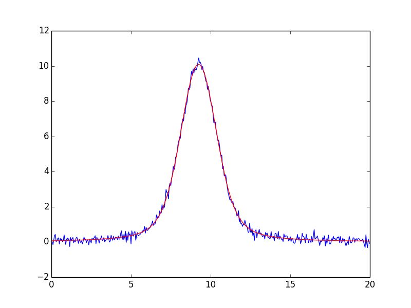
8.1   Peak-like models . . . . . . . . . . . . . . . . . . . . . . . . . . . . .                            .   .   .   .   .   .   .   .   .   .   .   .   .   .   .   .   51
     8.2   Linear and Polynomial Models . . . . . . . . . . . . . . . . . . . . .                                .   .   .   .   .   .   .   .   .   .   .   .   .   .   .   .   54
     8.3   Step-like models . . . . . . . . . . . . . . . . . . . . . . . . . . . . .                            .   .   .   .   .   .   .   .   .   .   .   .   .   .   .   .   55
     8.4   Exponential and Power law models . . . . . . . . . . . . . . . . . . .                                .   .   .   .   .   .   .   .   .   .   .   .   .   .   .   .   56
     8.5   User-defined Models . . . . . . . . . . . . . . . . . . . . . . . . . . .                             .   .   .   .   .   .   .   .   .   .   .   .   .   .   .   .   57
     8.6   Example 1: Fit Peaked data to Gaussian, Lorentzian, and Voigt profiles                                .   .   .   .   .   .   .   .   .   .   .   .   .   .   .   .   58
     8.7   Example 2: Fit data to a Composite Model with pre-defined models . .                                  .   .   .   .   .   .   .   .   .   .   .   .   .   .   .   .   61
     8.8   Example 3: Fitting Multiple Peaks – and using Prefixes . . . . . . . .                                .   .   .   .   .   .   .   .   .   .   .   .   .   .   .   .   62

9    Calculation of confidence intervals                                                                                                                                         67
     9.1 Method used for calculating confidence intervals        .   .   .   .   .   .   .   .   .   .   .   .   .   .   .   .   .   .   .   .   .   .   .   .   .   .   .   .   67
     9.2 A basic example . . . . . . . . . . . . . . . . .       .   .   .   .   .   .   .   .   .   .   .   .   .   .   .   .   .   .   .   .   .   .   .   .   .   .   .   .   67
     9.3 An advanced example . . . . . . . . . . . . . .         .   .   .   .   .   .   .   .   .   .   .   .   .   .   .   .   .   .   .   .   .   .   .   .   .   .   .   .   68
     9.4 Documentation of methods . . . . . . . . . . . .        .   .   .   .   .   .   .   .   .   .   .   .   .   .   .   .   .   .   .   .   .   .   .   .   .   .   .   .   71

10 Bounds Implementation                                                                                                                                                         75

11 Using Mathematical Constraints                                                                                                                                                77
   11.1 Overview . . . . . . . . . . . . . . . . . . . .     .   .   .   .   .   .   .   .   .   .   .   .   .   .   .   .   .   .   .   .   .   .   .   .   .   .   .   .   .   77
   11.2 Supported Operators, Functions, and Constants        .   .   .   .   .   .   .   .   .   .   .   .   .   .   .   .   .   .   .   .   .   .   .   .   .   .   .   .   .   77
   11.3 Using Inequality Constraints . . . . . . . . . .     .   .   .   .   .   .   .   .   .   .   .   .   .   .   .   .   .   .   .   .   .   .   .   .   .   .   .   .   .   78
   11.4 Advanced usage of Expressions in lmfit . . . .       .   .   .   .   .   .   .   .   .   .   .   .   .   .   .   .   .   .   .   .   .   .   .   .   .   .   .   .   .   79

Python Module Index                                                                                                                                                              81

Python Module Index                                                                                                                                                              83

Index                                                                                                                                                                            85

ii
Non-Linear Least-Squares Minimization and Curve-Fitting for Python, Release 0.8.3-94-g0ed9c2f
Lmfit provides a high-level interface to non-linear optimization and curve fitting problems for Python. Lmfit builds on
and extends many of the optimizatin algorithm of scipy.optimize, especially the Levenberg-Marquardt method
from scipy.optimize.leastsq().
Lmfit provides a number of useful enhancements to optimization and data fitting problems, including:
• Using Parameter objects instead of plain floats as variables. A Parameter has a value that can be varied
in the fit, have a fixed value, or have upper and/or lower bounds. A Parameter can even have a value that is
constrained by an algebraic expression of other Parameter values.
• Ease of changing fitting algorithms. Once a fitting model is set up, one can change the fitting algorithm used to
find the optimal solution without changing the objective function.
• Improved estimation of confidence intervals. While scipy.optimize.leastsq() will automatically cal-
culate uncertainties and correlations from the covariance matrix, the accuracy of these estimates are often ques-
tionable. To help address this, lmfit has functions to explicitly explore parameter space to determine confidence
levels even for the most difficult cases.
• Improved curve-fitting with the Model class. This extends the capabilities of
scipy.optimize.curve_fit(), allowing you to turn a function that models for your data into a
python class that helps you parametrize and fit data with that model.
• Many pre-built models for common lineshapes are included and ready to use.
The lmfit package is Free software, using an MIT license. The software and this document are works in progress. If
you are interested in participating in this effort please use the lmfit github repository.
CONTENTS 1Non-Linear Least-Squares Minimization and Curve-Fitting for Python, Release 0.8.3-94-g0ed9c2f 2 CONTENTS
CHAPTER

                                                                                                                   ONE

    GETTING STARTED WITH NON-LINEAR LEAST-SQUARES FITTING

The lmfit package is designed to provide simple tools to help you build complex fitting models for non-linear least-
squares problems and apply these models to real data. This section gives an overview of the concepts and describes
how to set up and perform simple fits. Some basic knowledge of Python, numpy, and modeling data are assumed.
To do a non-linear least-squares fit of a model to data or for a variety of other optimization problems, the main task
is to write an objective function that takes the values of the fitting variables and calculates either a scalar value to be
minimized or an array of values that is to be minimized in the least-squares sense. For many data fitting processes,
the least-squares approach is used, and the objective function should return an array of (data-model), perhaps scaled
by some weighting factor such as the inverse of the uncertainty in the data. For such a problem, the chi-square (χ2 )
statistic is often defined as:
                                                    N
                                                    X [y meas − y model (v)]2
                                                          i        i
                                             χ2 =
                                                     i
                                                                  2i

where yimeas is the set of measured data, yimodel (v) is the model calculation, v is the set of variables in the model to
be optimized in the fit, and i is the estimated uncertainty in the data.
In a traditional non-linear fit, one writes an objective function that takes the variable values and calculates the residual
yimeas − yimodel (v), or the residual scaled by the data uncertainties, [yimeas − yimodel (v)]/i , or some other weighting
factor. As a simple example, one might write an objective function like this:
def residual(vars, x, data, eps_data):
    amp = vars[0]
    phaseshift = vars[1]
    freq = vars[2]
    decay = vars[3]

     model = amp * sin(x * freq              + phaseshift) * exp(-x*x*decay)

     return (data-model)/eps_data

To perform the minimization with scipy.optimize, one would do:
from scipy.optimize import leastsq
vars = [10.0, 0.2, 3.0, 0.007]
out = leastsq(residual, vars, args=(x, data, eps_data))

Though it is wonderful to be able to use python for such optimization problems, and the scipy library is robust and
easy to use, the approach here is not terribly different from how one would do the same fit in C or Fortran. There are
several practical challenges to using this approach, including:
   1. The user has to keep track of the order of the variables, and their meaning – vars[0] is the amplitude, vars[2] is
      the frequency, and so on, although there is no intrinsic meaning to this order.

                                                                                                                          3
Non-Linear Least-Squares Minimization and Curve-Fitting for Python, Release 0.8.3-94-g0ed9c2f
2. If the user wants to fix a particular variable (not vary it in the fit), the residual function has to be altered to
have fewer variables, and have the corresponding constant value passed in some other way. While reasonable
for simple cases, this quickly becomes a significant work for more complex models, and greatly complicates
modeling for people not intimately familiar with the details of the fitting code.
3. There is no simple, robust way to put bounds on values for the variables, or enforce mathematical relationships
between the variables. In fact, those optimization methods that do provide bounds, require bounds to be set for
all variables with separate arrays that are in the same arbitrary order as variable values. Again, this is acceptable
for small or one-off cases, but becomes painful if the fitting model needs to change.
These shortcomings are really do solely to the use of traditional arrays of variables, as matches closely the imple-
mentation of the Fortran code. The lmfit module overcomes these shortcomings by using objects – a core reason for
wokring with Python. The key concept for lmfit is to use Parameter objects instead of plain floating point numbers
as the variables for the fit. By using Parameter objects (or the closely related Parameters – a dictionary of
Parameter objects), one can
1. forget about the order of variables and refer to Parameters by meaningful names.
2. place bounds on Parameters as attributes, without worrying about order.
3. fix Parameters, without having to rewrite the objective function.
4. place algebraic constraints on Parameters.
To illustrate the value of this approach, we can rewrite the above example as:
from lmfit import minimize, Parameters
def residual(params, x, data, eps_data):
amp = params['amp'].value
pshift = params['phase'].value
freq = params['frequency'].value
decay = params['decay'].value
model = amp * sin(x * freq + pshift) * exp(-x*x*decay)
return (data-model)/eps_data
params = Parameters()
params.add('amp', value=10)
params.add('decay', value=0.007)
params.add('phase', value=0.2)
params.add('frequency', value=3.0)
out = minimize(residual, params, args=(x, data, eps_data))
At first look, we simply replaced a list of values with a dictionary, accessed by name – not a huge improvement. But
each of the named Parameter in the Parameters object holds additional attributes to modify the value during the
fit. For example, Parameters can be fixed or bounded. This can be done during definition:
params = Parameters()
params.add('amp', value=10, vary=False)
params.add('decay', value=0.007, min=0.0)
params.add('phase', value=0.2)
params.add('frequency', value=3.0, max=10)
where vary=False will prevent the value from changing in the fit, and min=0.0 will set a lower bound on that
parameters value). It can also be done later by setting the corresponding attributes after they have been created:
params['amp'].vary = False
params['decay'].min = 0.10
4 Chapter 1. Getting started with Non-Linear Least-Squares FittingNon-Linear Least-Squares Minimization and Curve-Fitting for Python, Release 0.8.3-94-g0ed9c2f
Importantly, our objective function remains unchanged.
The params object can be copied and modified to make many user-level changes to the model and fitting process. Of
course, most of the information about how your data is modeled goes into the objective function, but the approach here
allows some external control; that is, control by the user performing the fit, instead of by the author of the objective
function.
Finally, in addition to the Parameters approach to fitting data, lmfit allows switching optimization methods with-
out changing the objective function, provides tools for writing fitting reports, and provides better determination of
Parameters confidence levels.
5Non-Linear Least-Squares Minimization and Curve-Fitting for Python, Release 0.8.3-94-g0ed9c2f 6 Chapter 1. Getting started with Non-Linear Least-Squares Fitting
CHAPTER

                                                                                                          TWO

                                                         DOWNLOADING AND INSTALLATION

2.1 Prerequisites

The lmfit package requires Python, Numpy, and Scipy. Scipy version 0.13 or higher is recommended, but extensive
testing on compatibility with various versions of scipy has not been done. Lmfit does work with Python 2.7, and 3.2
and 3.3. No testing has been done with Python 3.4, but as the package is pure Python, relying only on scipy and
numpy, no significant troubles are expected. The nose framework is required for running the test suite, and IPython
and matplotib are recommended. If Pandas is available, it will be used in portions of lmfit.

2.2 Downloads

The latest stable version of lmfit is available from PyPi.

2.3 Installation

If you have pip installed, you can install lmfit with:
pip install lmfit

or, if you have Python Setup Tools installed, you install lmfit with:
easy_install -U lmfit

or, you can download the source kit, unpack it and install with:
python setup.py install

2.4 Development Version

To get the latest development version, use:
git clone http://github.com/lmfit/lmfit-py.git

and install using:
python setup.py install

                                                                                                                 7
Non-Linear Least-Squares Minimization and Curve-Fitting for Python, Release 0.8.3-94-g0ed9c2f
2.5 Testing
A battery of tests scripts that can be run with the nose testing framework is distributed with lmfit in the tests folder.
These are routinely run on the development version. Running nosetests should run all of these tests to completion
without errors or failures.
Many of the examples in this documentation are distributed with lmfit in the examples folder, and should also run
for you. Many of these require
2.6 Acknowledgements
Many people have contributed to lmfit.
Matthew Newville wrote the original version and maintains the project.
Till Stensitzki wrote the improved estimates of confidence intervals, and
contributed many tests, bug fixes, and documentation.
Daniel B. Allan wrote much of the high level Model code, and many
improvements to the testing and documentation.
Antonino Ingargiola wrote much of the high level Model code and provided
many bug fixes.
J. J. Helmus wrote the MINUT bounds for leastsq, originally in
leastsqbounds.py, and ported to lmfit.
E. O. Le Bigot wrote the uncertainties package, a version of which is used
by lmfit.
Michal Rawlik added plotting capabilities for Models.
A. R. J. Nelson added differential_evolution, and greatly improved the code
in the docstrings.
Additional patches, bug fixes, and suggestions have come from Christoph
Deil, Francois Boulogne, Thomas Caswell, Colin Brosseau, nmearl,
Gustavo Pasquevich, Clemens Prescher, LiCode, and Ben Gamari.
The lmfit code obviously depends on, and owes a very large debt to the code
in scipy.optimize. Several discussions on the scipy-user and lmfit mailing
lists have also led to improvements in this code.
2.7 License
The LMFIT-py code is distribution under the following license:
Copyright, Licensing, and Re-distribution
-----------------------------------------
The LMFIT-py code is distribution under the following license:
Copyright (c) 2014 Matthew Newville, The University of Chicago
Till Stensitzki, Freie Universitat Berlin
Daniel B. Allen, Johns Hopkins University
Michal Rawlik, Eidgenossische Technische Hochschule, Zurich
Antonino Ingargiola, University of California, Los Angeles
A. R. J. Nelson, Australian Nuclear Science and Technology Organisation
Permission to use and redistribute the source code or binary forms of this
8 Chapter 2. Downloading and InstallationNon-Linear Least-Squares Minimization and Curve-Fitting for Python, Release 0.8.3-94-g0ed9c2f software and its documentation, with or without modification is hereby granted provided that the above notice of copyright, these terms of use, and the disclaimer of warranty below appear in the source code and documentation, and that none of the names of above institutions or authors appear in advertising or endorsement of works derived from this software without specific prior written permission from all parties. THE SOFTWARE IS PROVIDED "AS IS", WITHOUT WARRANTY OF ANY KIND, EXPRESS OR IMPLIED, INCLUDING BUT NOT LIMITED TO THE WARRANTIES OF MERCHANTABILITY, FITNESS FOR A PARTICULAR PURPOSE AND NONINFRINGEMENT. IN NO EVENT SHALL THE AUTHORS OR COPYRIGHT HOLDERS BE LIABLE FOR ANY CLAIM, DAMAGES OR OTHER LIABILITY, WHETHER IN AN ACTION OF CONTRACT, TORT OR OTHERWISE, ARISING FROM, OUT OF OR IN CONNECTION WITH THE SOFTWARE OR THE USE OR OTHER DEALINGS IN THIS SOFTWARE. 2.7. License 9
Non-Linear Least-Squares Minimization and Curve-Fitting for Python, Release 0.8.3-94-g0ed9c2f

10                                                      Chapter 2. Downloading and Installation
CHAPTER

                                                                                                           THREE

                                                                                            GETTING HELP

If you have questions, comments, or suggestions for LMFIT, please use the mailing list. This provides an on-line
conversation that is and archived well and can be searched well with standard web searches. If you find a bug with the
code or documentation, use the github issues Issue tracker to submit a report. If you have an idea for how to solve the
problem and are familiar with python and github, submitting a github Pull Request would be greatly appreciated.
If you are unsure whether to use the mailing list or the Issue tracker, please start a conversation on the mailing list.
That is, the problem you’re having may or may not be due to a bug. If it is due to a bug, creating an Issue from the
conversation is easy. If it is not a bug, the problem will be discussed and then the Issue will be closed. While one can
search through closed Issues on github, these are not so easily searched, and the conversation is not easily useful to
others later. Starting the conversation on the mailing list with “How do I do this?” or “Why didn’t this work?” instead
of “This should work and doesn’t” is generally preferred, and will better help others with similar questions. Of course,
there is not always an obvious way to decide if something is a Question or an Issue, and we will try our best to engage
in all discussions.

                                                                                                                     11
Non-Linear Least-Squares Minimization and Curve-Fitting for Python, Release 0.8.3-94-g0ed9c2f 12 Chapter 3. Getting Help
CHAPTER

                                                                                                           FOUR

                                                          FREQUENTLY ASKED QUESTIONS

A list of common questions.

4.1 How can I fit multi-dimensional data?

The fitting routines accept data arrays that are 1 dimensional and double precision. So you need to convert the data
and model (or the value returned by the objective function) to be one dimensional. A simple way to do this is to use
numpy’s numpy.ndarray.flatten(), for example:
def residual(params, x, data=None):
    ....
    resid = calculate_multidim_residual()
    return resid.flatten()

4.2 How can I fit multiple data sets?

As above, the fitting routines accept data arrays that are 1 dimensional and double precision. So you need to convert
the sets of data and models (or the value returned by the objective function) to be one dimensional. A simple way to
do this is to use numpy’s numpy.concatenate(). As an example, here is a residual function to simultaneously
fit two lines to two different arrays. As a bonus, the two lines share the ‘offset’ parameter:
      def fit_function(params, x=None, dat1=None, dat2=None): model1 = params[’offset’].value + x *
            params[’slope1’].value model2 = params[’offset’].value + x * params[’slope2’].value
           resid1 = dat1 - model1 resid2 = dat2 - model2 return numpy.concatenate((resid1, resid2))

4.3 How can I fit complex data?

As with working with multidimensional data, you need to convert your data and model (or the value returned by the
objective function) to be double precision floating point numbers. One way to do this would be to use a function like
this:
def realimag(array):
    return np.array([(x.real, x.imag) for x in array]).flatten()

to convert the complex array into an array of alternating real and imaginary values. You can then use this function on
the result returned by your objective function:

                                                                                                                   13
Non-Linear Least-Squares Minimization and Curve-Fitting for Python, Release 0.8.3-94-g0ed9c2f
def residual(params, x, data=None):
....
resid = calculate_complex_residual()
return realimag(resid)
4.4 Can I constrain values to have integer values?
Basically, no. None of the minimizers in lmfit support integer programming. They all (I think) assume that they
can make a very small change to a floating point value for a parameters value and see a change in the value to be
minimized.
4.5 How should I cite LMFIT?
See http://dx.doi.org/10.5281/zenodo.11813
14 Chapter 4. Frequently Asked QuestionsCHAPTER
FIVE
PARAMETER AND PARAMETERS
This chapter describes Parameter objects which is the key concept of lmfit.
A Parameter is the quantity to be optimized in all minimization problems, replacing the plain floating point number
used in the optimization routines from scipy.optimize. A Parameter has a value that can be varied in the fit
or have a fixed value, have upper and/or lower bounds. It can even have a value that is constrained by an algebraic
expression of other Parameter values. Since Parameters live outside the core optimization routines, they can be
used in all optimization routines from scipy.optimize. By using Parameter objects instead of plain variables,
the objective function does not have to be modified to reflect every change of what is varied in the fit. This simplifies
the writing of models, allowing general models that describe the phenomenon to be written, and gives the user more
flexibility in using and testing variations of that model.
Whereas a Parameter expands on an individual floating point variable, the optimization methods need an ordered
group of floating point variables. In the scipy.optimize routines this is required to be a 1-dimensional numpy
ndarray. For lmfit, where each Parameter has a name, this is replaced by a Parameters class, which works as
an ordered dictionary of Parameter objects, with a few additional features and methods. That is, while the concept
of a Parameter is central to lmfit, one normally creates and interacts with a Parameters instance that contains
many Parameter objects. The objective functions you write for lmfit will take an instance of Parameters as its
first argument.
5.1 The Parameter class
class Parameter(name=None[, value=None[, vary=True[, min=None[, max=None[, expr=None ]]]]])
create a Parameter object.
Parameters
• name (None or string – will be overwritten during fit if None.) – parameter name
• value – the numerical value for the parameter
• vary (boolean (True/False) [default True]) – whether to vary the parameter or not.
• min – lower bound for value (None = no lower bound).
• max – upper bound for value (None = no upper bound).
• expr (None or string) – mathematical expression to use to evaluate value during fit.
Each of these inputs is turned into an attribute of the same name.
After a fit, a Parameter for a fitted variable (that is with vary = True) may have its value attribute to hold the
best-fit value. Depending on the success of the fit and fitting algorithm used, it may also have attributes stderr and
correl.
15Non-Linear Least-Squares Minimization and Curve-Fitting for Python, Release 0.8.3-94-g0ed9c2f
stderr
the estimated standard error for the best-fit value.
correl
a dictionary of the correlation with the other fitted variables in the fit, of the form:
{'decay': 0.404, 'phase': -0.020, 'frequency': 0.102}
See Bounds Implementation for details on the math used to implement the bounds with min and max.
The expr attribute can contain a mathematical expression that will be used to compute the value for the Parameter at
each step in the fit. See Using Mathematical Constraints for more details and examples of this feature.
set(value=None[, vary=None[, min=None[, max=None[, expr=None ]]]])
set or update a Parameters value or other attributes.
Parameters
• name – parameter name
• value – the numerical value for the parameter
• vary – whether to vary the parameter or not.
• min – lower bound for value
• max – upper bound for value
• expr – mathematical expression to use to evaluate value during fit.
Each argument of set() has a default value of None, and will be set only if the provided value is not None. You
can use this to update some Parameter attribute without affecting others, for example:
p1 = Parameter('a', value=2.0)
p2 = Parameter('b', value=0.0)
p1.set(min=0)
p2.set(vary=False)
to set a lower bound, or to set a Parameter as have a fixed value.
Note that to use this approach to lift a lower or upper bound, doing::
p1.set(min=0)
.....
# now lift the lower bound
p1.set(min=None) # won't work! lower bound NOT changed
won't work -- this will not change the current lower bound. Instead
you'll have to use ``np.inf`` to remove a lower or upper bound::
# now lift the lower bound
p1.set(min=-np.inf) # will work!
Similarly, to clear an expression of a parameter, you need to pass an
empty string, not ``None``. You also need to give a value and
explicitly tell it to vary::
p3 = Parameter('c', expr='(a+b)/2')
p3.set(expr=None) # won't work! expression NOT changed
# remove constraint expression
p3.set(value=1.0, vary=True, expr='') # will work! parameter now unconstrained
16 Chapter 5. Parameter and ParametersNon-Linear Least-Squares Minimization and Curve-Fitting for Python, Release 0.8.3-94-g0ed9c2f
5.2 The Parameters class
class Parameters
create a Parameters object. This is little more than a fancy ordered dictionary, with the restrictions that:
1.keys must be valid Python symbol names, so that they can be used in expressions of mathematical con-
straints. This means the names must match [a-z_][a-z0-9_]* and cannot be a Python reserved word.
2.values must be valid Parameter objects.
Two methods are for provided for convenient initialization of a Parameters, and one for extracting
Parameter values into a plain dictionary.
add(name[, value=None[, vary=True[, min=None[, max=None[, expr=None ]]]]])
add a named parameter. This creates a Parameter object associated with the key name, with optional argu-
ments passed to Parameter:
p = Parameters()
p.add('myvar', value=1, vary=True)
add_many(self, paramlist)
add a list of named parameters. Each entry must be a tuple with the following entries:
name, value, vary, min, max, expr
This method is somewhat rigid and verbose (no default values), but can be useful when initially defining a
parameter list so that it looks table-like:
p = Parameters()
# (Name, Value, Vary, Min, Max, Expr)
p.add_many(('amp1', 10, True, None, None, None),
('cen1', 1.2, True, 0.5, 2.0, None),
('wid1', 0.8, True, 0.1, None, None),
('amp2', 7.5, True, None, None, None),
('cen2', 1.9, True, 1.0, 3.0, None),
('wid2', None, False, None, None, '2*wid1/3'))
pretty_print(oneline=False)
prints a clean representation on the Parameters. If oneline is True, the result will be printed to a single (long)
line.
valuesdict()
return an ordered dictionary of name:value pairs with the Paramater name as the key and Parameter value as
value.
This is distinct from the Parameters itself, as the dictionary values are not Parameter objects, just the
value. Using :method:‘valuesdict‘ can be a very convenient way to get updated values in a objective function.
dumps(**kws):
return a JSON string representation of the Parameter object. This can be saved or used to re-create or re-set
parameters, using the loads() method.
Optional keywords are sent json.dumps().
dump(file, **kws):
write a JSON representation of the Parameter object to a file or file-like object in file – really any object with
a write() method. Optional keywords are sent json.dumps().
loads(sval, **kws):
use a JSON string representation of the Parameter object in sval to set all parameter settins. Optional key-
words are sent json.loads().
5.2. The Parameters class 17Non-Linear Least-Squares Minimization and Curve-Fitting for Python, Release 0.8.3-94-g0ed9c2f
load(file, **kws):
read and use a JSON string representation of the Parameter object from a file or file-like object in file – really
any object with a read() method. Optional keywords are sent json.loads().
5.3 Simple Example
Using Parameters‘ and minimize() function (discussed in the next chapter) might look like this:
#!/usr/bin/env python
#
from lmfit import minimize, Parameters, Parameter, report_fit
import numpy as np
# create data to be fitted
x = np.linspace(0, 15, 301)
data = (5. * np.sin(2 * x - 0.1) * np.exp(-x*x*0.025) +
np.random.normal(size=len(x), scale=0.2) )
# define objective function: returns the array to be minimized
def fcn2min(params, x, data):
""" model decaying sine wave, subtract data"""
amp = params['amp'].value
shift = params['shift'].value
omega = params['omega'].value
decay = params['decay'].value
model = amp * np.sin(x * omega + shift) * np.exp(-x*x*decay)
return model - data
# create a set of Parameters
params = Parameters()
params.add('amp', value= 10, min=0)
params.add('decay', value= 0.1)
params.add('shift', value= 0.0, min=-np.pi/2., max=np.pi/2)
params.add('omega', value= 3.0)
# do fit, here with leastsq model
result = minimize(fcn2min, params, args=(x, data))
# calculate final result
final = data + result.residual
# write error report
report_fit(result.params)
# try to plot results
try:
import pylab
pylab.plot(x, data, 'k+')
pylab.plot(x, final, 'r')
pylab.show()
except:
pass
#
18 Chapter 5. Parameter and ParametersNon-Linear Least-Squares Minimization and Curve-Fitting for Python, Release 0.8.3-94-g0ed9c2f
Here, the objective function explicitly unpacks each Parameter value. This can be simplified using the Parameters
valuesdict() method, which would make the objective function fcn2min above look like:
def fcn2min(params, x, data):
""" model decaying sine wave, subtract data"""
v = params.valuesdict()
model = v['amp'] * np.sin(x * v['omega'] + v['shift']) * np.exp(-x*x*v['decay'])
return model - data
The results are identical, and the difference is a stylistic choice.
5.3. Simple Example 19Non-Linear Least-Squares Minimization and Curve-Fitting for Python, Release 0.8.3-94-g0ed9c2f 20 Chapter 5. Parameter and Parameters
CHAPTER

                                                                                                                  SIX

                                           PERFORMING FITS, ANALYZING OUTPUTS

As shown in the previous chapter, a simple fit can be performed with the minimize() function. For more sophis-
ticated modeling, the Minimizer class can be used to gain a bit more control, especially when using complicated
constraints or comparing results from related fits.

6.1 The minimize() function

The minimize() function is a wrapper around Minimizer for running an optimization problem. It takes an
objective function (the function that calculates the array to be minimized), a Parameters object, and several optional
arguments. See Writing a Fitting Function for details on writing the objective.
minimize(function, params[, args=None[, kws=None[, method=’leastsq’[, scale_covar=True[,
            iter_cb=None[, **fit_kws ]]]]]])
    find values for the params so that the sum-of-squares of the array returned from function is minimized.
           Parameters
                  • function (callable.) – function to return fit residual. See Writing a Fitting Function for
                    details.
                  • params (Parameters.) – a Parameters dictionary. Keywords must be strings that
                    match [a-z_][a-z0-9_]* and cannot be a python reserved word. Each value must be
                    Parameter.
                  • args (tuple) – arguments tuple to pass to the residual function as positional arguments.
                  • kws (dict) – dictionary to pass to the residual function as keyword arguments.
                  • method (string (default leastsq)) – name of fitting method to use. See Choosing Different
                    Fitting Methods for details
                  • scale_covar (bool (default True)) – whether to automatically scale covariance matrix
                    (leastsq only)
                  • iter_cb (callable or None) – function to be called at each fit iteration. See Using a Iteration
                    Callback Function for details.
                  • fit_kws (dict) – dictionary to pass             to   scipy.optimize.leastsq()               or
                    scipy.optimize.minimize().
           Returns MinimizerResult instance, which will contain the optimized parameter, and several
               goodness-of-fit statistics.
      On output, the params will be unchanged. The best-fit values, and where appropriate, estimated uncertainties and
      correlations, will all be contained in the returned MinimizerResult. See MinimizerResult – the optimization
      result for further details.

                                                                                                                      21
Non-Linear Least-Squares Minimization and Curve-Fitting for Python, Release 0.8.3-94-g0ed9c2f
For clarity, it should be emphasized that this function is simply a wrapper around Minimizer that runs a single
fit, implemented as:
fitter = Minimizer(fcn, params, fcn_args=args, fcn_kws=kws,
iter_cb=iter_cb, scale_covar=scale_covar, **fit_kws)
return fitter.minimize(method=method)
6.2 Writing a Fitting Function
An important component of a fit is writing a function to be minimized – the objective function. Since this function will
be called by other routines, there are fairly stringent requirements for its call signature and return value. In principle,
your function can be any python callable, but it must look like this:
func(params, *args, **kws):
calculate objective residual to be minimized from parameters.
Parameters
• params (Parameters.) – parameters.
• args – positional arguments. Must match args argument to minimize()
• kws – keyword arguments. Must match kws argument to minimize()
Returns residual array (generally data-model) to be minimized in the least-squares sense.
Return type numpy array. The length of this array cannot change between calls.
A common use for the positional and keyword arguments would be to pass in other data needed to calculate the
residual, including such things as the data array, dependent variable, uncertainties in the data, and other data structures
for the model calculation.
The objective function should return the value to be minimized. For the Levenberg-Marquardt algorithm from
leastsq(), this returned value must be an array, with a length greater than or equal to the number of fitting vari-
ables in the model. For the other methods, the return value can either be a scalar or an array. If an array is returned, the
sum of squares of the array will be sent to the underlying fitting method, effectively doing a least-squares optimization
of the return values.
Since the function will be passed in a dictionary of Parameters, it is advisable to unpack these to get numerical
values at the top of the function. A simple way to do this is with Parameters.valuesdict(), as with:
def residual(pars, x, data=None, eps=None):
# unpack parameters:
# extract .value attribute for each parameter
parvals = pars.valuesdict()
period = parvals['period']
shift = parvals['shift']
decay = parvals['decay']
if abs(shift) > pi/2:
shift = shift - sign(shift)*pi
if abs(period) < 1.e-10:
period = sign(period)*1.e-10
model = parvals['amp'] * sin(shift + x/period) * exp(-x*x*decay*decay)
if data is None:
return model
22 Chapter 6. Performing Fits, Analyzing OutputsNon-Linear Least-Squares Minimization and Curve-Fitting for Python, Release 0.8.3-94-g0ed9c2f
if eps is None:
return (model - data)
return (model - data)/eps
In this example, x is a positional (required) argument, while the data array is actually optional (so that the function
returns the model calculation if the data is neglected). Also note that the model calculation will divide x by the value
of the ‘period’ Parameter. It might be wise to ensure this parameter cannot be 0. It would be possible to use the bounds
on the Parameter to do this:
params['period'] = Parameter(value=2, min=1.e-10)
but putting this directly in the function with:
if abs(period) < 1.e-10:
period = sign(period)*1.e-10
is also a reasonable approach. Similarly, one could place bounds on the decay parameter to take values only between
-pi/2 and pi/2.
6.3 Choosing Different Fitting Methods
By default, the Levenberg-Marquardt algorithm is used for fitting. While often criticized, including the fact it finds
a local minima, this approach has some distinct advantages. These include being fast, and well-behaved for most
curve-fitting needs, and making it easy to estimate uncertainties for and correlations between pairs of fit variables, as
discussed in MinimizerResult – the optimization result.
Alternative algorithms can also be used by providing the method keyword to the minimize() function or
Minimizer.minimize() class as listed in the Table of Supported Fitting Methods.
Table of Supported Fitting Method, eithers:
Fitting Method method arg to minimize() or
Minimizer.minimize()
Levenberg-Marquardt leastsq
Nelder-Mead nelder
L-BFGS-B lbfgsb
Powell powell
Conjugate Gradient cg
Newton-CG newton
COBYLA cobyla
Truncated Newton tnc
Dogleg dogleg
Sequential Linear Squares slsqp
Programming
Differential Evolution differential_evolution
Note: The objective function for the Levenberg-Marquardt method must return an array, with more elements than
variables. All other methods can return either a scalar value or an array.
Warning: Much of this documentation assumes that the Levenberg-Marquardt method is the method used. Many
of the fit statistics and estimates for uncertainties in parameters discussed in MinimizerResult – the optimization
result are done only for this method.
6.3. Choosing Different Fitting Methods 23Non-Linear Least-Squares Minimization and Curve-Fitting for Python, Release 0.8.3-94-g0ed9c2f
6.4 MinimizerResult – the optimization result
class MinimizerResult(**kws)
An optimization with minimize() or Minimizer.minimize() will return a MinimizerResult object.
This is an otherwise plain container object (that is, with no methods of its own) that simply holds the results of
the minimization. These results will include several pieces of informational data such as status and error messages, fit
statistics, and the updated parameters themselves.
Importantly, the parameters passed in to Minimizer.minimize() will be not be changed. To to find the best-fit
values, uncertainties and so on for each parameter, one must use the MinimizerResult.params attribute.
params
the Parameters actually used in the fit, with updated values, stderr and correl.
var_names
ordered list of variable parameter names used in optimization, and useful for understanding the the values in
init_vals and covar.
covar
covariance matrix from minimization (leastsq only), with rows/columns using var_names.
init_vals
list of initial values for variable parameters using var_names.
nfev
number of function evaluations
success
boolean (True/False) for whether fit succeeded.
errorbars
boolean (True/False) for whether uncertainties were estimated.
message
message about fit success.
ier
integer error value from scipy.optimize.leastsq() (leastsq only).
lmdif_message
message from scipy.optimize.leastsq() (leastsq only).
nvarys
number of variables in fit Nvarys
ndata
number of data points: N
nfree ‘
degrees of freedom in fit: N − Nvarys
residual
residual array, return value of func(): Resid
chisqr PN
chi-square: χ2 = i [Residi ]2
redchi
reduced chi-square: χ2ν = χ2 /(N − Nvarys )
aic
Akaike Information Criterion statistic (see below)
24 Chapter 6. Performing Fits, Analyzing OutputsNon-Linear Least-Squares Minimization and Curve-Fitting for Python, Release 0.8.3-94-g0ed9c2f
bic
Bayesian Information Criterion statistic (see below).
6.4.1 Goodness-of-Fit Statistics
Table of Fit Results: These values, including the standard Goodness-of-Fit statistics, are all attributes of
the MinimizerResult object returned by minimize() or Minimizer.minimize().
Attribute Name Description / Formula
nfev number of function evaluations
nvarys number of variables in fit Nvarys
ndata number of data points: N
nfree ‘ degrees of freedom in fit: N − Nvarys
residual residual array, return value of func(): Resid
PN
chisqr chi-square: χ2 = i [Residi ]2
redchi reduced chi-square: χ2ν = χ2 /(N − Nvarys )
aic Akaike Information Criterion statistic (see below)
bic Bayesian Information Criterion statistic (see below)
var_names ordered list of variable parameter names used for init_vals and covar
covar covariance matrix (with rows/columns using var_names
init_vals list of initial values for variable parameters
Note that the calculation of chi-square and reduced chi-square assume that the returned residual function is scaled
properly to the uncertainties in the data. For these statistics to be meaningful, the person writing the function to be
minimized must scale them properly.
After a fit using using the leastsq() method has completed successfully, standard errors for the fitted variables and
correlations between pairs of fitted variables are automatically calculated from the covariance matrix. The standard
error (estimated 1σ error-bar) go into the stderr attribute of the Parameter. The correlations with all other variables
will be put into the correl attribute of the Parameter – a dictionary with keys for all other Parameters and values of
the corresponding correlation.
In some cases, it may not be possible to estimate the errors and correlations. For example, if a variable actually has no
practical effect on the fit, it will likely cause the covariance matrix to be singular, making standard errors impossible
to estimate. Placing bounds on varied Parameters makes it more likely that errors cannot be estimated, as being near
the maximum or minimum value makes the covariance matrix singular. In these cases, the errorbars attribute of
the fit result (Minimizer object) will be False.
6.4.2 Akaike and Bayesian Information Criteria
The MinimizerResult includes the tradtional chi-square and reduced chi-square statistics:
N
X
χ2 = ri2
i
χ2ν = = χ2 /(N − Nvarys )
where r is the residual array returned by the objective function (likely to be (data-model)/uncertainty for
data modeling usages), N is the number of data points (ndata), and Nvarys is number of variable parameters.
Also included are the Akaike Information Criterion, and Bayesian Information Criterion statistics, held in the aic and
bic attributes, respectively. These give slightly different measures of the relative quality for a fit, trying to balance
6.4. MinimizerResult – the optimization result 25Non-Linear Least-Squares Minimization and Curve-Fitting for Python, Release 0.8.3-94-g0ed9c2f
quality of fit with the number of variable parameters used in the fit. These are calculated as
aic = N ln(χ2 /N ) + 2Nvarys
bic = N ln(χ2 /N ) + ln(N ) ∗ Nvarys
Generally, when comparing fits with different numbers of varying parameters, one typically selects the model with low-
est reduced chi-square, Akaike information criterion, and/or Bayesian information criterion. Generally, the Bayesian
information criterion is considered themost conservative of these statistics.
6.5 Using a Iteration Callback Function
An iteration callback function is a function to be called at each iteration, just after the objective function is called. The
iteration callback allows user-supplied code to be run at each iteration, and can be used to abort a fit.
iter_cb(params, iter, resid, *args, **kws):
user-supplied function to be run at each iteration
Parameters
• params (Parameters.) – parameters.
• iter (integer) – iteration number
• resid (ndarray) – residual array.
• args – positional arguments. Must match args argument to minimize()
• kws – keyword arguments. Must match kws argument to minimize()
Returns residual array (generally data-model) to be minimized in the least-squares sense.
Return type None for normal behavior, any value like True to abort fit.
Normally, the iteration callback would have no return value or return None. To abort a fit, have this function return a
value that is True (including any non-zero integer). The fit will also abort if any exception is raised in the iteration
callback. When a fit is aborted this way, the parameters will have the values from the last iteration. The fit statistics
are not likely to be meaningful, and uncertainties will not be computed.
6.6 Using the Minimizer class
For full control of the fitting process, you’ll want to create a Minimizer object.
class Minimizer(function, params, fcn_args=None, fcn_kws=None, iter_cb=None, scale_covar=True,
**kws)
creates a Minimizer, for more detailed access to fitting methods and attributes.
Parameters
• function (callable.) – objective function to return fit residual. See Writing a Fitting Func-
tion for details.
• params (dict) – a dictionary of Parameters. Keywords must be strings that match
[a-z_][a-z0-9_]* and is not a python reserved word. Each value must be
Parameter.
• fcn_args (tuple) – arguments tuple to pass to the residual function as positional arguments.
• fcn_kws (dict) – dictionary to pass to the residual function as keyword arguments.
26 Chapter 6. Performing Fits, Analyzing OutputsNon-Linear Least-Squares Minimization and Curve-Fitting for Python, Release 0.8.3-94-g0ed9c2f
• iter_cb (callable or None) – function to be called at each fit iteration. See Using a Iteration
Callback Function for details.
• scale_covar – flag for automatically scaling covariance matrix and uncertainties to reduced
chi-square (leastsq only)
• kws (dict) – dictionary to pass as keywords to the underlying scipy.optimize method.
The Minimizer object has a few public methods:
minimize(method=’leastsq’, params=None, **kws)
perform fit using either leastsq() or scalar_minimize().
Parameters
• method (str.) – name of fitting method. Must be one of the naemes in Table of Supported
Fitting Methods
• params (Parameters or None) – a Parameters dictionary for starting values
Returns MinimizerResult object, containing updated parameters, fitting statistics, and infor-
mation.
Additonal keywords are passed on to the correspond leastsq() or scalar_minimize() method.
leastsq(params=None, scale_covar=True, **kws)
perform fit with Levenberg-Marquardt algorithm. Keywords will be passed directly to
scipy.optimize.leastsq(). By default, numerical derivatives are used, and the following argu-
ments are set:
leastsq() arg Default Value Description
xtol 1.e-7 Relative error in the approximate solution
ftol 1.e-7 Relative error in the desired sum of squares
maxfev 2000*(nvar+1) maximum number of function calls (nvar= # of
variables)
Dfun None function to call for Jacobian calculation
scalar_minimize(method=’Nelder-Mead’, params=None, hess=None, tol=None, **kws)
perform fit with any of the scalar minimization algorithms supported by scipy.optimize.minimize().
scalar_minimize() arg Default Value Description
method Nelder-Mead fitting method
tol 1.e-7 fitting and parameter tolerance
hess None Hessian of objective function
prepare_fit(**kws)
prepares and initializes model and Parameters for subsequent fitting. This routine prepares the conversion of
Parameters into fit variables, organizes parameter bounds, and parses, “compiles” and checks constrain
expressions. The method also creates and returns a new instance of a MinimizerResult object that contains
the copy of the Parameters that will actually be varied in the fit.
This method is called directly by the fitting methods, and it is generally not necessary to call this function
explicitly.
6.7 Getting and Printing Fit Reports
fit_report(result, modelpars=None, show_correl=True, min_correl=0.1)
generate and return text of report of best-fit values, uncertainties, and correlations from fit.
Parameters
6.7. Getting and Printing Fit Reports 27Non-Linear Least-Squares Minimization and Curve-Fitting for Python, Release 0.8.3-94-g0ed9c2f
• result – MinimizerResult object as returned by minimize().
• modelpars – Parameters with “Known Values” (optional, default None)
• show_correl – whether to show list of sorted correlations [True]
• min_correl – smallest correlation absolute value to show [0.1]
If the first argument is a Parameters object, goodness-of-fit statistics will not be included.
report_fit(result, modelpars=None, show_correl=True, min_correl=0.1)
print text of report from fit_report().
An example fit with report would be
#!/usr/bin/env python
#
from __future__ import print_function
from lmfit import Parameters, minimize, fit_report
from numpy import random, linspace, pi, exp, sin, sign
p_true = Parameters()
p_true.add('amp', value=14.0)
p_true.add('period', value=5.46)
p_true.add('shift', value=0.123)
p_true.add('decay', value=0.032)
def residual(pars, x, data=None):
vals = pars.valuesdict()
amp = vals['amp']
per = vals['period']
shift = vals['shift']
decay = vals['decay']
if abs(shift) > pi/2:
shift = shift - sign(shift)*pi
model = amp * sin(shift + x/per) * exp(-x*x*decay*decay)
if data is None:
return model
return (model - data)
n = 1001
xmin = 0.
xmax = 250.0
random.seed(0)
noise = random.normal(scale=0.7215, size=n)
x = linspace(xmin, xmax, n)
data = residual(p_true, x) + noise
fit_params = Parameters()
fit_params.add('amp', value=13.0)
fit_params.add('period', value=2)
fit_params.add('shift', value=0.0)
fit_params.add('decay', value=0.02)
out = minimize(residual, fit_params, args=(x,), kws={'data':data})
28 Chapter 6. Performing Fits, Analyzing OutputsNon-Linear Least-Squares Minimization and Curve-Fitting for Python, Release 0.8.3-94-g0ed9c2f
print(fit_report(out))
#
which would write out:
[[Fit Statistics]]
# function evals = 85
# data points = 1001
# variables = 4
chi-square = 498.812
reduced chi-square = 0.500
[[Variables]]
amp: 13.9121944 +/- 0.141202 (1.01%) (init= 13)
period: 5.48507044 +/- 0.026664 (0.49%) (init= 2)
shift: 0.16203677 +/- 0.014056 (8.67%) (init= 0)
decay: 0.03264538 +/- 0.000380 (1.16%) (init= 0.02)
[[Correlations]] (unreported correlations are < 0.100)
C(period, shift) = 0.797
C(amp, decay) = 0.582
C(amp, shift) = -0.297
C(amp, period) = -0.243
C(shift, decay) = -0.182
C(period, decay) = -0.150
6.7. Getting and Printing Fit Reports 29Non-Linear Least-Squares Minimization and Curve-Fitting for Python, Release 0.8.3-94-g0ed9c2f 30 Chapter 6. Performing Fits, Analyzing Outputs
CHAPTER
SEVEN
MODELING DATA AND CURVE FITTING
A common use of least-squares minimization is curve fitting, where one has a parametrized model function meant
to explain some phenomena and wants to adjust the numerical values for the model to most closely match some
data. With scipy, such problems are commonly solved with scipy.optimize.curve_fit(), which is a
wrapper around scipy.optimize.leastsq(). Since Lmfit’s minimize() is also a high-level wrapper around
scipy.optimize.leastsq() it can be used for curve-fitting problems, but requires more effort than using
scipy.optimize.curve_fit().
Here we discuss lmfit’s Model class. This takes a model function – a function that calculates a model for some data
– and provides methods to create parameters for that model and to fit data using that model function. This is closer in
spirit to scipy.optimize.curve_fit(), but with the advantages of using Parameters and lmfit.
In addition to allowing you turn any model function into a curve-fitting method, Lmfit also provides canonical defini-
tions for many known line shapes such as Gaussian or Lorentzian peaks and Exponential decays that are widely used
in many scientific domains. These are available in the models module that will be discussed in more detail in the
next chapter (Built-in Fitting Models in the models module). We mention it here as you may want to consult that list
before writing your own model. For now, we focus on turning python function into high-level fitting models with the
Model class, and using these to fit data.
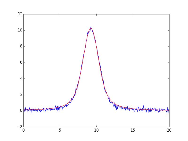
7.1 Example: Fit data to Gaussian profile
Let’s start with a simple and common example of fitting data to a Gaussian peak. As we will see, there is a buit-in
GaussianModel class that provides a model function for a Gaussian profile, but here we’ll build our own. We start
with a simple definition of the model function:
>>> from numpy import sqrt, pi, exp, linspace
>>>
>>> def gaussian(x, amp, cen, wid):
... return amp * exp(-(x-cen)**2 /wid)
...
We want to fit this objective function to data y(x) represented by the arrays y and x. This can be done easily wit
scipy.optimize.curve_fit():
>>> from scipy.optimize import curve_fit
>>>
>>> x = linspace(-10,10)
>>> y = y = gaussian(x, 2.33, 0.21, 1.51) + np.random.normal(0, 0.2, len(x))
>>>
>>> init_vals = [1, 0, 1] # for [amp, cen, wid]
>>> best_vals, covar = curve_fit(gaussian, x, y, p0=init_vals)
>>> print best_vals
31Non-Linear Least-Squares Minimization and Curve-Fitting for Python, Release 0.8.3-94-g0ed9c2f We sample random data point, make an initial guess of the model values, and run scipy.optimize.curve_fit() with the model function, data arrays, and initial guesses. The results returned are the optimal values for the parameters and the covariance matrix. It’s simple and very useful. But it misses the benefits of lmfit. To solve this with lmfit we would have to write an objective function. But such a function would be fairly simple (essentially, data - model, possibly with some weighting), and we would need to define and use appropriately named parameters. Though convenient, it is somewhat of a burden to keep the named parameter straight (on the other hand, with scipy.optimize.curve_fit() you are required to remember the parameter order). After doing this a few times it appears as a recurring pattern, and we can imagine automating this process. That’s where the Model class comes in. Model allows us to easily wrap a model function such as the gaussian function. This automatically generate the appropriate residual function, and determines the corresponding parameter names from the function signature itself: >>> from lmfit import Model >>> gmod = Model(gaussian) >>> gmod.param_names set(['amp', 'wid', 'cen']) >>> gmod.independent_vars) ['x'] The Model gmod knows the names of the parameters and the independent variables. By default, the first argument of the function is taken as the independent variable, held in independent_vars, and the rest of the functions positional arguments (and, in certain cases, keyword arguments – see below) are used for Parameter names. Thus, for the gaussian function above, the parameters are named amp, cen, and wid, and x is the independent variable – all taken directly from the signature of the model function. As we will see below, you can specify what the independent variable is, and you can add or alter parameters, too. The parameters are not created when the model is created. The model knows what the parameters should be named, but not anything about the scale and range of your data. You will normally have to make these parameters and assign initial values and other attributes. To help you do this, each model has a make_params() method that will generate parameters with the expected names: >>> params = gmod.make_params() This creates the Parameters but doesn’t necessarily give them initial values – again, the model has no idea what the scale should be. You can set initial values for parameters with keyword arguments to make_params(): >>> params = gmod.make_params(cen=5, amp=200, wid=1) or assign them (and other parameter properties) after the Parameters has been created. A Model has several methods associated with it. For example, one can use the eval() method to evaluate the model or the fit() method to fit data to this model with a Parameter object. Both of these methods can take explicit keyword arguments for the parameter values. For example, one could use eval() to calculate the predicted function: >>> x = linspace(0, 10, 201) >>> y = gmod.eval(x=x, amp=10, cen=6.2, wid=0.75) Admittedly, this a slightly long-winded way to calculate a Gaussian function. But now that the model is set up, we can also use its fit() method to fit this model to data, as with: >>> result = gmod.fit(y, x=x, amp=5, cen=5, wid=1) Putting everything together, the script to do such a fit (included in the examples folder with the source code) is: #!/usr/bin/env python # from numpy import sqrt, pi, exp, linspace, loadtxt 32 Chapter 7. Modeling Data and Curve Fitting
You can also read