COSMO-Model Tutorial March 2018
←
→
Page content transcription
If your browser does not render page correctly, please read the page content below
COSMO-Model Tutorial

March 2018

     Working with the COSMO-Model

                 Practical Exercises

for NWP Mode, RCM Mode, and COSMO-ART

For NWP Mode:    Ulrich Schättler, Ulrich Blahak, Michael Baldauf

For RCM Mode:    Burkhardt Rockel, Merja Tölle, Andreas Will,
                 Ivonne Anders, Christian Steger
For COSMO-ART:   Bernhard Vogel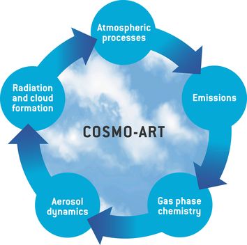
i

Contents

1 Installation of the COSMO-Model Package                                                                1
  1.1   Introduction . . . . . . . . . . . . . . . . . . . . . . . . . . . . . . . . . . . . . . . . .    1
        1.1.1   The COSMO-Model Package . . . . . . . . . . . . . . . . . . . . . . . . . . .             1
        1.1.2   External Libraries needed by the COSMO-Model Package . . . . . . . . . . .                2
        1.1.3   Computer Platforms for the COSMO-Model Package . . . . . . . . . . . . . .                4
        1.1.4   Necessary Data to run the System . . . . . . . . . . . . . . . . . . . . . . . .          4
        1.1.5   Practical Informations for these Exercises . . . . . . . . . . . . . . . . . . . .        5
  1.2   Installation of the External Libraries . . . . . . . . . . . . . . . . . . . . . . . . . . .      5
        1.2.1   DWD GRIB1 Library . . . . . . . . . . . . . . . . . . . . . . . . . . . . . . .           5
        1.2.2   ECMWF GRIB-API . . . . . . . . . . . . . . . . . . . . . . . . . . . . . . . .            7
        1.2.3   NetCDF . . . . . . . . . . . . . . . . . . . . . . . . . . . . . . . . . . . . . . .      9
  1.3   Installation of the Programs . . . . . . . . . . . . . . . . . . . . . . . . . . . . . . . .      9
        1.3.1   The source code . . . . . . . . . . . . . . . . . . . . . . . . . . . . . . . . . .       9
        1.3.2   Adaptation of Fopts and the Makefile . . . . . . . . . . . . . . . . . . . . . . 10
        1.3.3   Compiling and linking the binary . . . . . . . . . . . . . . . . . . . . . . . . . 10
  1.4   Installation of the reference-data . . . . . . . . . . . . . . . . . . . . . . . . . . . . . 10
  1.5   Installation of the starter package for the climate mode . . . . . . . . . . . . . . . . . 11
  1.6   Exercises . . . . . . . . . . . . . . . . . . . . . . . . . . . . . . . . . . . . . . . . . . . 12

2 Preparing External, Initial and Boundary Data                                                          13
  2.1   Namelist Input for the INT2LM . . . . . . . . . . . . . . . . . . . . . . . . . . . . . . 13
  2.2   External Data . . . . . . . . . . . . . . . . . . . . . . . . . . . . . . . . . . . . . . . . 13
  2.3   The Model Domain . . . . . . . . . . . . . . . . . . . . . . . . . . . . . . . . . . . . . 14
        2.3.1   The Horizontal Grid . . . . . . . . . . . . . . . . . . . . . . . . . . . . . . . . 14
        2.3.2   Choosing the Vertical Grid . . . . . . . . . . . . . . . . . . . . . . . . . . . . 14
        2.3.3   The Reference Atmosphere . . . . . . . . . . . . . . . . . . . . . . . . . . . . 15
CONTENTS ii
2.3.4 Summary of Namelist Group LMGRID . . . . . . . . . . . . . . . . . . . . . . . 16
2.4 Coarse Grid Model Data . . . . . . . . . . . . . . . . . . . . . . . . . . . . . . . . . . 17
2.4.1 Possible Driving Models . . . . . . . . . . . . . . . . . . . . . . . . . . . . . . 17
2.4.2 Specifying Regular Grids . . . . . . . . . . . . . . . . . . . . . . . . . . . . . . 18
2.4.3 Specifying the GME Grid . . . . . . . . . . . . . . . . . . . . . . . . . . . . . 18
2.4.4 Specifying the ICON Grid . . . . . . . . . . . . . . . . . . . . . . . . . . . . . 19
2.5 Specifying Data Characteristics . . . . . . . . . . . . . . . . . . . . . . . . . . . . . . 20
2.5.1 External Parameters for the COSMO-Model . . . . . . . . . . . . . . . . . . . 20
2.5.2 External Parameters for the Driving Model . . . . . . . . . . . . . . . . . . . 20
2.5.3 Input Data from the Driving Model . . . . . . . . . . . . . . . . . . . . . . . 20
2.5.4 COSMO Grid Output Data . . . . . . . . . . . . . . . . . . . . . . . . . . . . 21
2.6 Parameters to Control the INT2LM Run . . . . . . . . . . . . . . . . . . . . . . . . . 22
2.6.1 Forecast Time, Domain Decomposition and Driving Model . . . . . . . . . . . 22
2.6.2 Basic Control Parameters . . . . . . . . . . . . . . . . . . . . . . . . . . . . . 22
2.6.3 Main Switch to choose NWP- or RCM-Mode . . . . . . . . . . . . . . . . . . 23
2.6.4 Additional Switches Interesting for the RCM-Mode . . . . . . . . . . . . . . . 23
2.7 Exercises . . . . . . . . . . . . . . . . . . . . . . . . . . . . . . . . . . . . . . . . . . . 25
2.7.1 NWP-Mode . . . . . . . . . . . . . . . . . . . . . . . . . . . . . . . . . . . . . 25
2.7.2 RCM-Mode . . . . . . . . . . . . . . . . . . . . . . . . . . . . . . . . . . . . . 25
3 Running the COSMO-Model 27
3.1 Namelist Input for the COSMO-Model . . . . . . . . . . . . . . . . . . . . . . . . . . 27
3.1.1 The Model Domain . . . . . . . . . . . . . . . . . . . . . . . . . . . . . . . . . 28
3.1.2 Basic Control Variables . . . . . . . . . . . . . . . . . . . . . . . . . . . . . . 28
3.1.3 Settings for the Dynamics . . . . . . . . . . . . . . . . . . . . . . . . . . . . . 29
3.1.4 Settings for the Physics . . . . . . . . . . . . . . . . . . . . . . . . . . . . . . 30
3.1.5 Settings for the I/O . . . . . . . . . . . . . . . . . . . . . . . . . . . . . . . . 30
3.1.6 Settings for the Diagnostics . . . . . . . . . . . . . . . . . . . . . . . . . . . . 31
3.2 Exercises . . . . . . . . . . . . . . . . . . . . . . . . . . . . . . . . . . . . . . . . . . . 31
3.2.1 NWP-Mode . . . . . . . . . . . . . . . . . . . . . . . . . . . . . . . . . . . . . 31
3.2.2 RCM-Mode . . . . . . . . . . . . . . . . . . . . . . . . . . . . . . . . . . . . . 32
CONTENTSCONTENTS iii
4 Visualizing COSMO-Model Output using GrADS 33
4.1 Introduction . . . . . . . . . . . . . . . . . . . . . . . . . . . . . . . . . . . . . . . . . 33
4.2 The data descriptor file . . . . . . . . . . . . . . . . . . . . . . . . . . . . . . . . . . 33
4.3 The gribmap program . . . . . . . . . . . . . . . . . . . . . . . . . . . . . . . . . . . 37
4.4 A Sample GrADS Session . . . . . . . . . . . . . . . . . . . . . . . . . . . . . . . . . 37
4.4.1 Drawing a Map Background . . . . . . . . . . . . . . . . . . . . . . . . . . . . 43
4.4.2 Use of GrADS in Batch mode . . . . . . . . . . . . . . . . . . . . . . . . . . . 45
4.5 Helpful Tools: . . . . . . . . . . . . . . . . . . . . . . . . . . . . . . . . . . . . . . . . 45
4.5.1 wgrib . . . . . . . . . . . . . . . . . . . . . . . . . . . . . . . . . . . . . . . . 46
4.5.2 grib2ctl and gribapi2ctl . . . . . . . . . . . . . . . . . . . . . . . . . . . . 47
4.5.3 grib_api Tools . . . . . . . . . . . . . . . . . . . . . . . . . . . . . . . . . . . 47
4.5.4 Exercise . . . . . . . . . . . . . . . . . . . . . . . . . . . . . . . . . . . . . . . 47
5 Postprocessing and visualization of NetCDF files 49
5.1 Introduction . . . . . . . . . . . . . . . . . . . . . . . . . . . . . . . . . . . . . . . . . 49
5.2 ncdump . . . . . . . . . . . . . . . . . . . . . . . . . . . . . . . . . . . . . . . . . . . 49
5.3 CDO and NCO . . . . . . . . . . . . . . . . . . . . . . . . . . . . . . . . . . . . . . . 50
5.4 ncview . . . . . . . . . . . . . . . . . . . . . . . . . . . . . . . . . . . . . . . . . . . . 50
5.5 Further tools for visualization and manipulation of NetCDF data . . . . . . . . . . . 51
5.6 ETOOL . . . . . . . . . . . . . . . . . . . . . . . . . . . . . . . . . . . . . . . . . . . 51
5.7 Exercises . . . . . . . . . . . . . . . . . . . . . . . . . . . . . . . . . . . . . . . . . . . 51
6 Running Idealized Test Cases 53
6.1 General remarks . . . . . . . . . . . . . . . . . . . . . . . . . . . . . . . . . . . . . . 53
6.1.1 Visualization . . . . . . . . . . . . . . . . . . . . . . . . . . . . . . . . . . . . 55
6.1.2 gnuplot . . . . . . . . . . . . . . . . . . . . . . . . . . . . . . . . . . . . . . . 55
6.2 Exercises . . . . . . . . . . . . . . . . . . . . . . . . . . . . . . . . . . . . . . . . . . . 56
7 Troubleshooting for the COSMO-Model 59
7.1 Compiling and Linking . . . . . . . . . . . . . . . . . . . . . . . . . . . . . . . . . . . 59
7.2 Troubleshooting in NWP-Mode . . . . . . . . . . . . . . . . . . . . . . . . . . . . . . 60
7.2.1 Running INT2LM . . . . . . . . . . . . . . . . . . . . . . . . . . . . . . . . . 60
7.2.2 Running the COSMO-Model . . . . . . . . . . . . . . . . . . . . . . . . . . . 61
7.3 Troubleshooting in RCM-Mode . . . . . . . . . . . . . . . . . . . . . . . . . . . . . . 62
CONTENTSCONTENTS iv
Appendix A The Computer System at DWD 63
A.1 Available Plattforms at DWD . . . . . . . . . . . . . . . . . . . . . . . . . . . . . . . 63
A.2 The Batch System for the Cray . . . . . . . . . . . . . . . . . . . . . . . . . . . . . . 64
A.3 Cray Run-Scripts for the Programs . . . . . . . . . . . . . . . . . . . . . . . . . . . . 64
A.3.1 Scripts for COSMO-model real case simulations and INT2LM . . . . . . . . . 64
A.3.2 Scripts for idealized COSMO-model simulations . . . . . . . . . . . . . . . . . 69
Appendix B The Computer System at DKRZ 73
B.1 Available Plattforms at DKRZ . . . . . . . . . . . . . . . . . . . . . . . . . . . . . . 73
B.2 The Batch System for the mistral . . . . . . . . . . . . . . . . . . . . . . . . . . . . . 73
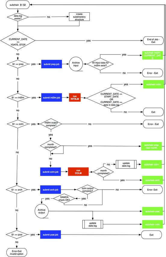
B.3 Script environment for running the COSMO-CLM in a chain . . . . . . . . . . . . . 74
B.3.1 The scripts . . . . . . . . . . . . . . . . . . . . . . . . . . . . . . . . . . . . . 74
B.3.2 The environment variables . . . . . . . . . . . . . . . . . . . . . . . . . . . . . 76
B.3.3 Extensions . . . . . . . . . . . . . . . . . . . . . . . . . . . . . . . . . . . . . 77
B.3.4 Running the CCLM chain . . . . . . . . . . . . . . . . . . . . . . . . . . . . . 78
B.3.5 The directory structure . . . . . . . . . . . . . . . . . . . . . . . . . . . . . . 78
B.3.6 Remarks . . . . . . . . . . . . . . . . . . . . . . . . . . . . . . . . . . . . . . . 78
Appendix C Necessary Files and Data for the NWP Mode 81
C.1 Availability of Source Codes and Data . . . . . . . . . . . . . . . . . . . . . . . . . . 81
C.2 External Parameters . . . . . . . . . . . . . . . . . . . . . . . . . . . . . . . . . . . . 82
C.3 Driving Data . . . . . . . . . . . . . . . . . . . . . . . . . . . . . . . . . . . . . . . . 87
Appendix D Necessary Files and Data for the Climate Mode 89
D.1 The Source Codes . . . . . . . . . . . . . . . . . . . . . . . . . . . . . . . . . . . . . 90
D.2 External Parameters . . . . . . . . . . . . . . . . . . . . . . . . . . . . . . . . . . . . 90
D.3 Initial and Boundary Data . . . . . . . . . . . . . . . . . . . . . . . . . . . . . . . . . 90
D.4 Preprocessor and model system overview . . . . . . . . . . . . . . . . . . . . . . . . . 91
CONTENTS1
Chapter 1
Installation of the COSMO-Model
Package
1.1 Introduction
1.1.1 The COSMO-Model Package
The COSMO-Model Package is a regional numerical weather prediction system. It is based on the
COSMO-Model, a nonhydrostatic limited-area atmospheric prediction model. Besides the forecast
model itself, a number of additional components such as data assimilation, interpolation of boundary
conditions from the driving model, and pre- and postprocessing utilities are required to run the
COSMO-Model in numerical weather prediction-mode (NWP-mode), in climate mode (RCM-mode)
or for idealized case studies. Since some time it is also possible to run an online coupled module
for aerosols and reactive trace gases together with the COSMO-Model (COSMO-ART). The source
code for the COSMO-Model Package consists of the following two programs:
• The interpolation program INT2LM
The INT2LM interpolates data from different data sets to the rotated latitude-longitude grid
of the COSMO-Model. Thus it provides the initial and / or boundary data necessary to run
the COSMO-Model. Data from the global models ICON (ICOsahedral, Non-hydrostatic: new
global model of DWD since January 2015), GME (icosahedral hydrostatic: old global model
of DWD), IFS (spectral model of ECMWF) and the regional COSMO-Model itself can be
processed directly. For the climate mode, processing of a common data format from global
data sets has been implemented. Thus, data from ECHAM5, ERA15, ERA40, NCEP and
some other models can be processed. An extra pre-pre-processor is needed to convert these
data to the common data format.
• The nonhydrostatic limited-area COSMO-Model
The COSMO-Model is a nonhydrostatic limited-area atmospheric prediction model. It has
been designed for both operational numerical weather prediction (NWP) and various scientific
applications on the meso-β and meso-γ scale. Between 2002 and 2006, a climate mode has
been developed and implemented, which also allows for long-term simulations and regional
climate calculations. The NWP-mode and the climate mode share the same source code. With
every major release, the diverging developments are unified again. This code basis is also used
to couple COSMO-ART to the model. But note, that COSMO-ART requires additional source
code, which is provided by the Karlsruhe Institute for Technology (KIT).
The COSMO-Model is based on the primitive thermo-hydrodynamical equations describing
COSMO-Model Tutorial CHAPTER 1. INSTALLATION OF THE COSMO-MODEL PACKAGE2 1.1 Introduction
compressible flow in a moist atmosphere. The model equations are formulated in rotated
geographical coordinates and a generalized terrain-following height coordinate. A variety of
physical processes are taken into account by parameterization schemes. Also included in the
model is a continuous data assimilation scheme for the atmospheric variables based on the
nudging method.
The purpose of this tutorial is to give you some practical experience in installing and running the
COSMO-Model Package. Exercises can be carried out on the supercomputers at DWD and / or
DKRZ, resp. The principal steps of the installation can directly be transferred to other systems.
1.1.2 External Libraries needed by the COSMO-Model Package
There are some tasks, for which the COSMO-Model package needs external libraries. All libraries
are implemented with appropriate ifdefs and their usage can be avoided. Note, that if a special
ifdef is not set, the corresponding tasks cannot be performed by the programs. The tasks, the
associated libraries and the ifdef-names are listed below.
Data Input and Output
Two data formats are implemented in the package to read and write data from or to disk: GRIB
and NetCDF.
• GRIB (GRIdded Binary) is a standard defined by the World Meteorological Organization
(WMO) for the exchange of processed data in the form of grid point values expressed in
binary form. GRIB coded data consist of a continuous bit-stream made of a sequence of octets
(1 octet = 8 bits). There are 2 versions of GRIB, which are actually used at the moment.
GRIB1 exists since the end of 1990ies and still is used at most weather services. GRIB2 is the
new standard, which is only used at a few centers up to now, among them the DWD. The
COSMO-Model can work with both GRIB versions, but needs different libraries for GRIB1
and GRIB2.
• NetCDF (Network Common Data Form) is a set of software libraries and machine-independent
data formats that support the creation, access, and sharing of array-oriented scientific data.
NetCDF files contain the complete information about the dependent variables, the history
and the fields themselves.
For more information on NetCDF see http://www.unidata.ucar.edu.
To work with the formats described above the following libraries are implemented in the COSMO-
Model package:
• The DWD GRIB1 library libgrib1.a
DWD provides a library to pack and unpack data using the GRIB1 format. This library also
containes the C-routines for performing the input and output for the programs. It cannot
work with the new GRIB2 standard.
To activate the interface routines to this library and to link it, the programs have to be
compiled with the preprocessor directive GRIBDWD.
• The ECMWF GRIB_API libraries libgrib_api.a, libgrib_api_f90.a
ECMWF developed an application programmers interface (API) to pack and unpack GRIB1
as well as GRIB2 format, the grib_api. It has been implemented and can be used now for
GRIB2 format from version INT2LM 2.01 and COSMO-Model 5.03 on. Please note that the
CHAPTER 1. INSTALLATION OF THE COSMO-MODEL PACKAGE COSMO-Model Tutorial1.1 Introduction 3
COSMO-Model system uses GRIB_API only for GRIB2. GRIB1 is still treated with the
DWD GRIB1 library. To activate grib_api and to link the two corresponding libraries, the
programs have to be compiled with the preprocessor directive GRIBAPI.
• The NetCDF library libnetcdf.a
A special library, the NetCDF-library, is necessary to write and read data using the NetCDF
format. This library also contains routines for manipulating and visualizing the data (nco-
routines). Additionally, CDO-routines written at the Max-Planck-Institute for Meteorology in
Hamburg may be used. These routines provide additional features like the harmonics or the
vorticity of the wind field.
To activate the NetCDF interface routines and to link the corresponding library, the programs
have to be compiled with the preprocessor directive NETCDF.
Observation Processing
In data assimilation mode it is necessary to process observation data, which is also done using
NetCDF files. Therefore, the libnetcdf.a is also necessary for running the COSMO-Model with
observation processing. To activate the data assimilation mode, the COSMO-Model has to be com-
piled with the preprocessor directive NUDGING. If this directive is not specified, the source code for
the data assimilation mode is not compiled. It is not possible to run data assimilation then.
Synthetic Satellite Images
Since Version 3.7 (February 2004) the COSMO-Model contains an interface to the RTTOV7-library
(Radiative Transfer Model). This interface has been developed at the DLR Institute for Atmospheric
Physics in Oberpfaffenhofen. Together with the RTTOV7-library it is possible to compute synthetic
satellite images (brightness temperatures and radiances) derived from model variables for various
instruments from the satellites Meteosat5-7 and Meteosat Second Generation.
Later, this interface has been expanded to work with newer RTTOV versions, RTTOV9 and RT-
TOV10. The RTTOV libraries are developed and maintained by UKMO et al. in the framework of
the ESA NWP-SAF. They are modified at DWD to be used in parallel programs. To use the RTTOV-
libraries, a license is necessary. For getting this license, please contact nwpsaf@metoffice.gov.uk.
• RTTOV7: librttov7.a
To activate the interface for RTTOV7, the model has to be compiled with the preprocessor
directive RTTOV7.
• RTTOV9: librttov_ifc.a, librttov9.3.a, librttov9.3_parallel.a
In Version 4.18 also an interface to the newer RTTOV9-library has been installed. Besides the
model-specific interface there is an additional model-independent interface, mo_rttov_ifc,
which is also available from an external library librttov_ifc.a. For using RTTOV9, two
additional external libraries librttov9.3_parallel.a and librttov9.3.a are also necessary.
To activate the interfaces for RTTOV9, the model has to be compiled with the preprocessor
directive RTTOV9.
• RTTOV10: librttov10.2.a, libradiance10.2.a, libhrit.a
COSMO-Model 5.0 also contains the interface for the RTTOV10 libraries. To activate the in-
terfaces for RTTOV10, the model has to be compiled with the preprocessor directive RTTOV10.
Since COSMO-Model 5.03 on, a modified version of the libradiance10.2.a plus an additional
library libhrit.a is necessary.
Note that only one of these libraries can be activated. If none of the directives RTTOV7, RTTOV9
or RTTOV10 is specified, the RTTOV-libraries are not necessary. The computation of the synthetic
satellite images is not possible then.
COSMO-Model Tutorial CHAPTER 1. INSTALLATION OF THE COSMO-MODEL PACKAGE4 1.1 Introduction 1.1.3 Computer Platforms for the COSMO-Model Package For practical work, the libraries and programs have to be installed on a computer system. You should have some knowledge about Unix / Linux, Compilers and Makefiles for these exercises. INT2LM and the COSMO-Model are implemented for distributed memory parallel computers using the Message Passing Interface (MPI), but can also be installed on sequential computers, where MPI is not available. For that purpose, a file dummy_mpi.f90 has to be compiled and linked with the programs. A Makefile is provided with the source codes, where the compiler call, the options and the necessary libraries can be specified. All the codes have already been ported to different computer platforms and may easily be adapted to other systems. If you want to port the libraries and programs, you have to adapt the compiler and linker options in the Makefiles (see Sections 1.2.1 and 1.3.2) and the machine dependent parts in the run-scripts (see Appendices A-3 and / or B-3, resp.) 1.1.4 Necessary Data to run the System Besides the source codes of the COSMO-package and the libraries, data are needed to perform runs of the COSMO-Model. There are three categories of necessary data: External Parameter Files External parameters are used to describe the surface of the earth. These data include the orography and the land-sea-mask. Also, several parameters are needed to specify the dominant land use of a grid box like the soil type or the plant cover. For fixed domain sizes and resolutions some external parameter files for the COSMO-Model are available. For the NWP community these data are usually provided in GRIB-format, while the CLM-Community prefers the NetCDF format. External parameter data sets can be generated for any domain on the earth. Depending on the raw data sets available up to now, the highest resolution possible is about 2 km (0.02 degrees). At DWD there is a tool EXTPAR for creating the external parameters. The CLM-Community uses a web interface called WebPEP as a graphical user interface to extpar. More information on this issue can be found in the COSMO-Model documentation. Boundary Conditions Because the COSMO-Model is a regional system, it needs boundary data from a driving model. For the NWP-mode it is possible to use the ICON (or old GME) and the IFS as driving models. Also, the COSMO-Model data can be used as boundary data for a higher resolution COSMO run. The boundary data are interpolated to the COSMO-Model grid with the INT2LM. For the climate mode, several driving models are possible. A pre-pre-processor transforms their out- put into a common format, which can be processed by the INT2LM. See additional documentation from the CLM-Community for this mode. CHAPTER 1. INSTALLATION OF THE COSMO-MODEL PACKAGE COSMO-Model Tutorial
1.2 Installation of the External Libraries                                                          5

Initial Conditions

In an operational NWP-mode, initial conditions for the COSMO-Model are produced by Data
Assimilation. Included in the COSMO-Model is the nudging procedure, that nudges the model
state towards available observations. For normal test runs and case studies, the initial data can also
be derived from the driving model using the INT2LM. In general, this is also the way it is done for
climate simulations since data assimilation is not used then.

1.1.5     Practical Informations for these Exercises

For practical work during these exercises, you need informations about the use of the computer
systems and from where you can access the necessary files and data. Depending on whether you run
the NWP- or the RCM-mode, these informations are differing. Please take a look at the following
Appendices:

  A: The Computer System at DWD
     To get informations on how to use DWD’s supercomputer and run test jobs using the NWP-
     runscripts.

  B: The Computer System at DKRZ
     To get informations on how to use DKRZ’s supercomputer and run test jobs using the RCM-
     runscripts.

  C: Necessary Files and Data for the NWP-Mode
     To get informations from where you can access the source code and the data for the NWP-
     exercises.

  D: Necessary Files and Data for the RCM-Mode
     To get informations from where you can access the source code and the data for the RCM-
     exercises.

1.2      Installation of the External Libraries

1.2.1     DWD GRIB1 Library

Introduction

The GRIB1 library has two major tasks:

    • First, it has to pack the meteorological fields into GRIB1 code and vice versa. Because GRIB1
      coded data consists of a continuous bit stream, this library has to deal with the manipulation
      of bits and bytes, which is not straightforward in Fortran.

    • The second task is the reading and writing of these bit streams. The corresponding routines
      are written in C, because this usually has a better performance than Fortran-I/O.

The bit manipulation and the Fortran-C interface (which is not standardized across different plat-
forms) makes the GRIB1 library a rather critical part of the COSMO-Model Package, because its
implementation is machine dependent.

COSMO-Model Tutorial                         CHAPTER 1. INSTALLATION OF THE COSMO-MODEL PACKAGE
6 1.2 Installation of the External Libraries
Source code of the DWD grib library
The source code of the grib library and a Makefile are contained in the compressed tar-file
DWD-libgrib1_.tar.gz (or .bz2). By unpacking (tar xvf DWD-libgrib1_.tar) a
directory DWD-libgrib1_ is created that contains a README and subdirectories include
and source. In the include-subdirectory several header files are contained, that are included dur-
ing the compilation to the source files. The source-subdirectory contains the source code and a
Makefile.
For a correct treatment of the Fortran-C-Interface and for properly working with bits and bytes, the
Makefile has to be adapted to the machine used. For the compiler-calls and -flags, several variables
are defined which can be commented / uncommented as needed. For the changes in the source code,
implementations are provided for some machines with ifdefs. If there is no suitable definition /
implementation, this has to be added.
Adaptation of the Makefile
In the Makefile, the following variables and commands have to be adjusted according to your needs:
LIBPATH Directory, to which the library is written (this directory again is needed in the
Makefiles of INT2LM and COSMO-Model).
INCDIR ../include.
AR This is the standard Unix archiving utility. If compiling and archiving on one
computer, but for another platform (like working on a front-end and compiling
code for a NEC SX machine), this also should be adapted.
FTN Call to the Fortran compiler.
FCFLAGS Options for compiling the Fortran routines in fixed form. Here the -Dxxx must
be set.
F90FLAGS Options for compiling the Fortran routines in free form.
CC Call to the C-Compilers (should be cc most everywhere).
CCFLAGS Options for compiling the C routines.
Here the -Dxxx must be set to choose one of the ifdef variants.
Big Endian / Little Endian
Unix computers, which are available today, use so-called Big Endian processors, which means that
they number the bits in a byte from 0 to 7. Typical PC-processors (Intel et al.) do it the other way
round and number the bits from 7 to 0. Because of this, the byte-order has to be swapped when
using a PC or a Linux machine. This byte-swapping is implemented in the grib library and can be
switched on by defining -D__linux__.
Compiling and creating the library
make or also make all compiles the routines and creates the library libgrib1.a in LIBPATH. On
most machines you can also compile the routines in parallel by using the GNU-make with the
command gmake -j np, where np gives the number of processors to use (typically 8).
CHAPTER 1. INSTALLATION OF THE COSMO-MODEL PACKAGE COSMO-Model Tutorial1.2 Installation of the External Libraries 7
Running programs using the DWD GRIB1 library
All programs that are doing GRIB1 I/O, have to be linked with the library libgrib1.a. There are
two additional issues that have to be considered when running programs using this GRIB1 library:
• DWD still uses a GRIB1 file format, where all records are starting and ending with additional
bytes, the so-called controlwords. An implementation of the GRIB1 library is prepared that
also deals with pure GRIB1 files, that do not have these controlwords. But still we guarantee
correct execution only, if these controlwords are used. To ensure this you have to set the
environment variable
export LIBDWD_FORCE_CONTROLWORDS=1.
in all your run-scripts.
• Another environment variable has to be set, if INT2LM is interpolating GME data that are
using ASCII bitmap files:
export LIBDWD_BITMAP_TYPE=ASCII.
(because this library can also deal with binary bitmap files, which is the default).
1.2.2 ECMWF GRIB-API
Introduction
ECMWF provides a library to pack and unpack GRIB data, the grib_api, which can be used for
GRIB1 and GRIB2. The approach, how data is coded to and decoded from GRIB messages is rather
different compared to DWD GRIB1 library. While the DWD GRIB1-library provides interfaces to
code and decode the full GRIB message in one step, the grib_api uses the so-called key/value
approach, where the single meta data could be set. In addition to these interface routines (available
for Fortran and for C), there are some command line tools to provide an easy way to check and
manipulate GRIB data from the shell. Please note that the COSMO-Model supports GRIB_API
only for GRIB2, not for GRIB1.
For more information on grib_api we refer to the ECMWF web page:
https://software.ecmwf.int/wiki/display/GRIB/Home.
Installation
The source code for the grib_api can be downloaded from the ECMWF web page
https://software.ecmwf.int/wiki/display/GRIB/Releases.
Please refer to the README for installing the grib_api libraries, which is done with a configure-
script. Check the following settings:
• Installation directory: create the directory where to install grib_api:
mkdir /e/uhome/trngxyx/grib_api
COSMO-Model Tutorial CHAPTER 1. INSTALLATION OF THE COSMO-MODEL PACKAGE8 1.2 Installation of the External Libraries
• If you do not use standard compilers (e.g. on DWD’s Cray system), you can either set environ-
ment variables or give special options to the configure-script. If you work on a standard linux
machine with the gcc compiler environment, you do not need to specify these environment
variables.
– export CC=/opt/cray/craype/2.5.7/bin/cc
– export CFLAGS=’-O2 -hflex_mp=conservative -h fp_trap’
– export LDFLAGS=’-K trap=fp’
– export F77=’/opt/cray/craype/2.5.7/bin/ftn’
– export FFLAGS=’-O2 -hflex_mp=conservative -h fp_trap’
– export FC=’/opt/cray/craype/2.5.7/bin/ftn’
– export FCFLAGS=’-O2 -hflex_mp=conservative -h fp_trap’
• grib_api can make use of optional jpeg-packing of the GRIB records, but this requires the
installation of additional packages. Because INT2LM and the COSMO-Model do not use these
optional packaging, use of jpeg can be disabled during the configure-step with the option
–disable-jpeg
• To use static linked libraries and binaries, you should give the configure option
–enable-shared=no.
./configure –prefix=/your/install/dir –disable-jpeg –enable-shared=no
After the configuration has finished, the grib_api library can be build with make and then make
install.
Note, that it is not necessary to set the environment variables mentioned above for the DWD GRIB1
library.
Usage of GRIB_API in the COSMO-Modell System
In addition to the GRIB_API libraries, some definition files are necessary at runtime. The set
of definition files provided by EMCWF can be extended by an own installation, and DWD has
chosen to do so for a more convenient implementation and use within the DWD-models. Which files
shall be used during model run is specified via an environment variable GRIB_DEFINITION_PATH.
This has to be set before the model is started:
export GRIB_DEFINITION_PATH=/your/path/definitions.edzw:/your/path/definitions
definitions.edzw is a directory containing the DWD definitions, which is distributed together
with the model system. Note that both paths have to be specified in this environment variable,
and that definitions.edzw has to be the first! More explanations on the definition files is given
during the exercises.
CHAPTER 1. INSTALLATION OF THE COSMO-MODEL PACKAGE COSMO-Model Tutorial1.3 Installation of the Programs 9
1.2.3 NetCDF
NetCDF is a freely available library for reading and writing scientific data sets. If the library is
not yet installed on your system, you can get the source code and documentation (this includes a
description how to install the library on different platforms) from
http://www.unidata.ucar.edu/software/netcdf/index.html
Please make sure that the F90 package is also installed, since the model reads and writes data
through the F90 NetCDF functions.
For this training course, the path to access the NetCDF library on the used computer system is
already included in the Fopts and / or Makefile.
1.3 Installation of the Programs
1.3.1 The source code
The files int2lm_yymmdd_x.y.tar.gz and cosmo_yymmdd_x.y.tar.gz (or .bz2) contain the source
codes of the INT2LM and the COSMO-Model, resp. yymmdd describes the date in the form "Year-
Month-Day" and x.y gives the version number as in the DWD Version Control System (VCS).
Since between major model updates the code is developed in parallel by the DWD and the CLM-
Community, the code names are slightly different for COSMO-CLM where a suffix clmz is added
(int2lm_yymmdd_x.y_clmz and cosmo_yymmdd_x.y_clmz), where z stands for an additional sub-
version number.
By unpacking (tar xvf int2lm_yymmdd_x.y.tar or tar xvf cosmo_yymmdd_x.y.tar) a directory
int2lm_yymmdd_x.y (or cosmo_yymmdd_x.y) is created which contains a Makefile together with
some associated files and (for the NWP Versions) some example run-scripts to set the Namelist
Parameters for certain configurations and to start the programs.
DOCS Contains a short documentation of the changes in version x.
Fopts Definition of the compiler options and also directories of libraries.
LOCAL Contains several examples of Fopts-files for different computers.
Makefile For compiling and linking the programs.
runxxx2yy Scripts to set the Namelist values for a configuration from model xxx to ap-
plication yy and start the program.
src Subdirectory for the source code.
obj Subdirectory where the object files are written.
Dependencies Definition of the dependencies between the different source files.
Objfiles Definition of the object files.
work Subdirectory for intermediate files.
Generally, only the Fopts part needs to be adapted by the user for different computer systems.
COSMO-Model Tutorial CHAPTER 1. INSTALLATION OF THE COSMO-MODEL PACKAGE10 1.4 Installation of the reference-data
1.3.2 Adaptation of Fopts and the Makefile
In Fopts, the variables for compiler-calls and -options and the directories for the used libraries have
to be adapted. In the subdirectory LOCAL, some example Fopts-files are given for different hardware
platforms and compilers. If there is nothing suitable, the variables have to be defined as needed.
F90 Call to the Fortran (90) compiler.
LDPAR Call to the linker to create a parallel binary.
LDSEQ Call to the linker to create a sequential binary without using the Message
Passing Interface (MPI).
PROGRAM The binary can be given a special name.
COMFLG1
... Options for compiling the Fortran routines of the COSMO-Model.
COMFLG4
LDFLG Options for linking.
AR Name of the archiving utility. This usually is ar, but when using the NEC
cross compiler it is sxar.
LIB Directories and names of the used external libraries.
1.3.3 Compiling and linking the binary
With the Unix command make exe (or just make), the programs are compiled and all object files
are linked to create the binaries. On most machines you can also compile the routines in parallel by
using the GNU-make with the command gmake -j np, where np gives the number of processors to
use (typically 8).
1.4 Installation of the reference-data
The file reference_data_5.05.tar(.bz2) contains an ICON reference data set together with the
ASCII output, created on the Cray XC40 of DWD. Included are ICON output data from the 07th of
July, 2015, 12 UTC, for up to 12 hours. These data are only provided for a special region over central
Europe. By unpacking (tar xvf reference_data_5.05.tar) the following directory structure is
created:
COSMO_2_input Binary input data for the COSMO-Model (2.8 km resolution; only
selected data sets available for comparison with your results)
COSMO_2_output Binary output data from the COSMO-Model (2.8 km resolution;
only selected data sets available for comparison with your results)
cosmo_2_output_ascii ASCII reference output from the COSMO-Model (2.8 km resolu-
tion) together with a run-script run_cosmo_2.
CHAPTER 1. INSTALLATION OF THE COSMO-MODEL PACKAGE COSMO-Model Tutorial1.5 Installation of the starter package for the climate mode 11
COSMO_7_input Binary input data for the COSMO-Model (7 km resolution; only
selected data sets available for comparison with your results)
COSMO_7_output Binary output data from the COSMO-Model (7 km resolution; only
selected data sets available for comparison with your results)
cosmo_7_output_ascii ASCII reference output from the COSMO-Model (7 km resolution)
together with a run-script run_cosmo_7.
ICON_2015070712_sub Binary ICON GRIB2 input data for the INT2LM and necessary
ICON external parameter and grib files (partly in NetCDF format).
int2lm_2_output_ascii ASCII reference output from the INT2LM run that transforms the
COSMO-Model 7 km data to the 2.8 km grid together with a run-
script run_cosmo7_2_cosmo2.
int2lm_7_output_ascii ASCII reference output from the INT2LM run that transforms the
ICON data data to the 7 km COSMO-Model grid together with a
run-script run_icon_2_cosmo7.
README More information on the reference data set.
The characteristics of this data set are: Start at 07. July 2015, 12 UTC + 12 hours.
Application Resolution grid size startlat_tot startlon_tot
km / degrees
COSMO-7 7 / 0.0625 129×161×40 -5.0 -4.0
COSMO-2 2.8 / 0.025 121×141×50 -3.5 -3.5
1.5 Installation of the starter package for the climate mode
For the climate simulation, all the necessary code and input files to start working with the COSMO-
CLM are included in the starter package which is available on the CLM-Community web page. After
unpacking the archive (tar -xzvf cclm-sp.tgz) you find the source code, initial and boundary
data, external parameters and run scripts as described in Appendix B and D. Note that the starter
package requires the netCDF4 library linked with HDF5 and zip libraries and extended by the
Fortran netCDF package. The netCDF4 package comes with the programs ncdump and nccopy. If
you are using the starter package on another computer than mistral make sure that these programs
are installed correctly1 .
The compilation of the libraries and binaries is very similar to that for the NWP mode (Sections
1.2–1.3). In this course, we need to compile the INT2LM and COSMO-CLM binaries. The NetCDF
library is already available on the mistral computer. The GRIB library is not used in the course.
An additional package of some small auxiliary fortran programs is needed which is called CFU.
In all cases you have to type ’make’ in the respective subdirectory to compile the codes. For INT2LM
and COSMO-CLM you have to adopt the Fopts file and set your working directory (SPDIR) first. An
initalization script called init.sh helps with these adoptions. It is therefore useful to run this script
once directly after unpacking the whole package. On computer systems other than the mistral at
1
software available from http://www.unidata.ucar.edu/software/netcdf/index.html
COSMO-Model Tutorial CHAPTER 1. INSTALLATION OF THE COSMO-MODEL PACKAGE12 1.6 Exercises
DKRZ you have to be careful to make the necessary additional changes in the Fopts and Makefile.
Some of these options are already available in the files.
More information on the setup of the model can be found on the CLM-Community webpage. In
Model → Support, you can find the starter package, the WebPEP tool for generating external data
files, a namelist tool with detailed information on the namelist parameters of the model and links
to the bug reporting system and technical pages (RedC) and some other utilities.
1.6 Exercises
NWP-Mode:
EXERCISE:
Install the DWD GRIB1-library, the ECMWF grib_api, the INT2LM and the COSMO-
Model on your computer and make a test run using the reference data set. For that you
have to do:
• Copy the source files to your home directory and the reference data set to your
work- or scratch-directory (see Appendix C-1).
• Install the libraries and programs according to Sections 1.2.1, 1.2.2, 1.3 and 1.4.
• Run the INT2LM and the COSMO-Model for (at least) the 7 km resolution. Copy
the corresponding run-scripts to the directories where you installed INT2LM and
the COSMO-Model, resp.. You only have to change some directory names and the
machine you want to run on (hopefully). See Appendix A-3 for an explanation of
the run-scripts.
RCM-Mode:
EXERCISE:
Install the COSMO-CLM starter package on your computer and compile the necessary
programs. For that you have to do:
• Copy the starter package to your scratch-directory (see Appendix D).
• Install the library and programs according to Sections 1.3 and 1.5.
CHAPTER 1. INSTALLATION OF THE COSMO-MODEL PACKAGE COSMO-Model Tutorial13
Chapter 2
Preparing External, Initial and
Boundary Data
In this lesson you should prepare the initial and boundary data for a COSMO-Model domain of
your choice. You will learn how to specify some important Namelist variables for the INT2LM.
2.1 Namelist Input for the INT2LM
The execution of INT2LM can be controlled by 6 NAMELIST groups:
CONTRL parameters for the model run
GRID_IN specifying the domain and the size of the driving model grid
LMGRID specifying the domain and the size of the LM grid
DATA controlling the grib input and output
PRICTR controlling grid point output
All NAMELIST groups have to appear in the input file INPUT in the order given above. Default
values are set for all parameters, you only have to specify values, that have to be different from the
default. The NAMELIST variables can be specified by the user in the run-script for the INT2LM,
which then creates the INPUT file. See Appendices A.3 (NWP) and / or B.3 (RCM) for details on
the run scripts.
2.2 External Data
Before you can start a test run, you have to specify a domain for the COSMO-Model and get some
external parameters for this domain. How the domain is specified is explained in detail in Sect. 2.3.
Because of interpolation reasons the external parameter must contain at least one additional row of
grid points on all four sides of the model domain. The domain for the external parameters can be
larger than the domain for which the COSMO-Model will be run. The INT2LM cuts out the proper
domain then.
For the first exercises, you have to take one of the external data sets specified in Appendix C.2
(for NWP) or Appendix D.2 (for RCM). In the future, if you want to work with different domains,
you can contact DWD or the CLM-Community to provide you an external parameter set for your
domain.
COSMO-Model Tutorial CHAPTER 2. PREPARING EXTERNAL, INITIAL AND BOUNDARY DATA14 2.3 The Model Domain
2.3 The Model Domain
This section explains the variables of the Namelist group LMGRID and gives some theoretical back-
ground.
To specify the domain of your choice, you have to choose the following parameters:
1. The lower left grid point of the domain in rotated coordinates.
2. The horizontal resolution in longitudinal and latitudinal direction in degrees.
3. The size of the domain in grid points.
4. The geographical coordinates of the rotated north pole, to specify the rotation
(or the angles of rotation for the domain).
5. The vertical resolution by specifying the vertical coordinate parameters.
All these parameters can be determined by Namelist variables of the Namelist group LMGRID. In the
following the variables and their meaning is explained.
Note: For describing the bigger domain of the external parameters, you have to specify values for
1) - 4) above. A vertical resolution cannot be given for the external parameters, because they are
purely horizontal.
2.3.1 The Horizontal Grid
The COSMO-Model uses a rotated spherical coordinate system, where the poles are moved and can
be positioned such that the equator runs through the centre of the model domain. Thus, problems
resulting from the convergence of the meridians can be minimized for any limited area model domain
on the globe.
Within the area of the chosen external parameter data set, you can specify any smaller area for your
tests. Please note that you have to choose at least one grid point less on each side of the domain of
the external parameters because of interpolation reasons.
The horizontal grid is specified by setting the following Namelist variables. Here we show an example
for a domain in central Europe.
startlat_tot = -17.0, lower left grid point in rotated coordinates
startlon_tot = -12.5,
dlon=0.0625, dlat=0.0625, horizontal resolution of the model
ielm_tot=225, jelm_tot=269, horizontal size of the model domain in grid points
pollat = 40.0, pollon = -170.0, geographical coordinates of rotated north pole
(or: angles of rotation for the domain)
2.3.2 Choosing the Vertical Grid
To specify the vertical grid, the number of the vertical levels must be given together with their
position in the atmosphere. This can be done by the Namelist variables kelm_tot and by defining the
list of vertical coordinate parameters σ1 , . . . , σke (which have the Namelist variable vcoord_d(:)).
CHAPTER 2. PREPARING EXTERNAL, INITIAL AND BOUNDARY DATA COSMO-Model Tutorial2.3 The Model Domain 15
This is the most difficult part of setting up the model domain, because a certain knowledge about
the vertical grid is necessary. The COSMO-Model equations are formulated using a terrain-following
coordinate system with a generalized vertical coordinate. Please refer to the Scientific Documen-
tation (Part I: Dynamics and Numerics) for a full explanation of the vertical coordinate system.
For practical applications, three different options are offered by INT2LM to specify the vertical
coordinate. The options are chosen by the Namelist variable ivctype:
1. A pressure based coordinate (deprecated: should not be used any more)
The σ values are running from 0 (top of the atmosphere) to 1 (surface),
e.g. σ1 = 0.02, . . . , σke = 1.0.
2. A height based coordinate (standard):
The σ values are given in meters above sea level,
e.g. σ1 = 23580.4414, . . . , σke = 0.0.
3. A height based SLEVE (Smooth LEvel VErtical) coordinate:
The σ values are specified as in 2. In addition some more parameters are necessary. Please
refer to the documentation for a full specification of the SLEVE coordinate.
All these coordinates are hybrid coordinates, i.e. they are terrain following in the lower part of the
atmosphere and change back to a pure z-coordinate (flat horizontal lines with a fixed height above
mean sea level) at a certain height. This height is specified by the Namelist variable vcflat. vcflat
has to be specified according to the chosen vertical coordinate parameters (pressure based or height
based).
Most operational applications in extra-tropical areas now use 40 levels together with coarser hor-
izontal resolutions (up to 7 km) and 50 levels for very high horizontal resolution runs (about 2-3
km). A special setup with higher model domains is available for tropical areas, to better catch
high-reaching convection.
Summary of the Namelist variables regarding the vertical grid:
ivctype=2, to choose the type of the vertical coordinate
vcoord_d=σ1 , . . . , σke , list of vertical coordinate parameters to specify the
vertical grid structure
vcflat=11430.0, height, where levels change back to z-system
kelm_tot=40, vertical size of the model domain in grid points
Because the specification of the vertical coordinate parameters σk is not straightforward, INT2LM
offers pre-defined sets of coordinate parameters for ivctype=2 and kelm_tot=40 or kelm_tot=50.
Then the list of vertical coordinate parameters vcoord_d= σ1 , . . . , σke and vcflat are set by the
INT2LM.
2.3.3 The Reference Atmosphere
In the COSMO-Model, pressure p is defined as the sum of a base state (p0 ) and deviations from this
base state (p0 ). The base state (or reference state) p0 is prescribed to be horizontally homogeneous,
i.e. depending only on the height above the surface, is time invariant and hydrostatically balanced.
To define the base state, some other default values like sea surface pressure (pSL ) and sea surface
temperature (TSL ) are needed. With these specifications, the reference atmosphere for the COSMO-
Model is computed. For a full description of the reference atmosphere, please refer to the Scientific
Documentation (Part I: Dynamics and Numerics)
COSMO-Model Tutorial CHAPTER 2. PREPARING EXTERNAL, INITIAL AND BOUNDARY DATA16 2.3 The Model Domain
The COSMO-Model offers 2 different types for the reference atmosphere.
1: For the first reference atmosphere a constant rate of increase in temperature with the loga-
rithm of pressure is assumed. Therefore, the reference atmosphere has a finite height and the
top of the model domain has to be positioned below this maximum value in order to avoid
unrealistical low reference temperatures in the vicinity of the upper boundary.
2: The second reference atmosphere is based on a temperature profile which allows a higher
model top:
−z
t0 (z) = (t0sl − ∆t) + ∆t · exp ,
hscal
where z = hhl(k) is the height of a model grid point. If this option is used, also the values for
∆t = delta_t and hscal = h_scal have to be set.
Which type of reference atmosphere is used, is chosen by the Namelist variable irefatm = 1/2.
Some additional characteristics of the chosen atmosphere can also be set. For further details see
the User Guide for the INT2LM (Part V: Preprocessing, Sect. 7.3: Specifying the Domain and the
Model Grid).
The values of the reference atmosphere are calculated analytically on the model half levels. These are
the interfaces of the vertical model layers, for which most atmospheric variables are given. Because
the values are also needed on the full levels (i.e. the model layers), they also have to be computed
there. For the first reference atmosphere (irefatm=1) there are 2 different ways how to compute
the values on the full levels. This is controlled by the namelist switch lanalyt_calc_t0p0:
- lanalyt_calc_t0p0=.FALSE.
The values on the full levels are computed by averaging the values from the half levels. This
has to be set for the Leapfrog dynamical core (l2tls=.FALSE. in the COSMO-Model) or
for the old Runge-Kutta fast waves solver (l2tls=.TRUE. and (itype_fast_waves=1 in the
COSMO-Model).
- lanalyt_calc_t0p0=.TRUE.
The values on the full levels are also calculated analytically on the full levels. This has to be
set for the new Runge-Kutta fast waves solver (l2tls=.TRUE. and (itype_fast_waves=2 in
the COSMO-Model).
For irefatm=2 the values on the full levels are always calculated analytically.
2.3.4 Summary of Namelist Group LMGRID
Example of the Namelist variables in the group LMGRID, that are necessary for these exercises:
&LMGRID
startlat_tot = -17.0, startlon_tot = -12.5,
dlon=0.0625, dlat=0.0625,
ielm_tot=225, jelm_tot=269, kelm_tot=40,
pollat = 40.0, pollon = -170.0,
ivctype=2,
irefatm=2,
delta_t=75.0,
h_scal=10000.0,
/
CHAPTER 2. PREPARING EXTERNAL, INITIAL AND BOUNDARY DATA COSMO-Model Tutorial2.4 Coarse Grid Model Data 17
Example for 50 vertical levels in extra-tropical regions:
vcoord_d= 22000.00, 21000.00, 20028.57, 19085.36, 18170.00, 17282.14, 16421.43,
15587.50, 14780.00, 13998.57, 13242.86, 12512.50, 11807.14, 11126.43,
10470.00, 9837.50, 9228.57, 8642.86, 8080.00, 7539.64, 7021.43,
6525.00, 6050.00, 5596.07, 5162.86, 4750.00, 4357.14, 3983.93,
3630.00, 3295.00, 2978.57, 2680.36, 2400.00, 2137.14, 1891.43,
1662.50, 1450.00, 1253.57, 1072.86, 907.50, 757.14, 621.43,
500.00, 392.50, 298.57, 217.86, 150.00, 94.64, 51.43,
20.00, 0.00,
Example for 50 vertical levels in tropical regions:
vcoord_d= 30000.00, 28574.09, 27198.21, 25870.74, 24590.12, 23354.87, 22163.61,
21014.99, 19907.74, 18840.66, 17812.60, 16822.44, 15869.14, 14951.68,
14069.12, 13220.53, 12405.03, 11621.78, 10869.96, 10148.82, 9457.59,
8795.59, 8162.12, 7556.52, 6978.19, 6426.50, 5900.89, 5400.80,
4925.71, 4475.11, 4048.50, 3645.43, 3265.45, 2908.13, 2573.08,
2259.90, 1968.23, 1697.72, 1448.06, 1218.94, 1010.07, 821.21,
652.12, 502.61, 372.52, 261.72, 170.16, 100.00, 50.00,
20.00, 0.00,
2.4 Coarse Grid Model Data
This section explains most variables of the Namelist group GRID_IN.
2.4.1 Possible Driving Models
With the INT2LM it is possible to interpolate data from several driving models to the COSMO
grid. Up to now the following input models are supported in NWP mode:
• ICON: New non-hydrostatic global model from DWD with an icosahedral model grid
• GME: Old hydrostatic global model from DWD with an icosahedral model grid
• IFS: Global spectral model from ECMWF; data is delivered on a Gaussian grid
• COSMO: Data from a coarser COSMO-Model run can be used to drive higher resolution runs
In the RCM mode, additional driving models are possible:
• NCEP: Data from the National Center for Environmental Prediction (USA)
• ERA40, ERA-Interim or ERA20C: Data from the ECMWF Reanalysis
COSMO-Model Tutorial CHAPTER 2. PREPARING EXTERNAL, INITIAL AND BOUNDARY DATA18 2.4 Coarse Grid Model Data
• JRA55: Data from the Japan Meteorological Agency global reanalysis
• ECHAM5/6: Data from the global model of MPI Hamburg
• HADAM: Data from the Hadley Centre, (UK)
• REMO: Data from the regional climate model REMO, MPI Hamburg.
• several CMIP5 GCMs: CGCM3, HadGEM, CNRM, EC-EARTH, Miroc5, CanESM2
The data of these models are pre-pre-processed, to have the data in a common format, which can
be processed by the INT2LM.
2.4.2 Specifying Regular Grids
The Namelist group GRID_IN specifies the characteristics of the grid of the driving model chosen.
Most input models use a rectangular grid which can be specified by the following Namelist variables:
startlat_in_tot latitude of lower left grid point of total input domain
startlon_in_tot longitude of lower left grid point of total input domain
dlon_in longitudinal resolution of the input grid
dlat_in latitudinal resolution of the input grid
ie_in_tot longitudinal grid point size
je_in_tot latitudinal grid point size
ke_in_tot vertical grid point size
pollat_in geographical latitude of north pole (if applicable; or angle of rotation)
pollon_in geographical longitude of north pole (if applicable; or angle of rotation)
2.4.3 Specifying the GME Grid
The GME has a special horizontal grid derived from the icosahedron. The characteristics of the
GME grid are specified with the variables:
ni_gme= ni stands for number of intersections of a great circle between two points of
the icosahedron and determines the horizontal resolution.
i3e_gme= vertical levels of GME
In the last years the resolution of GME has been increased several times. Depending on the date
you are processing, the above Namelist variables have to be specified according to the following
table:
Date ni_gme i3e_gme
before 02.02.2010, 12 UTC 192 40
02.02.2010, 12 UTC - 29.02.2012, 00 UTC 256 60
29.02.2012, 12 UTC - 20.01.2014, 00 UTC 384 60
CHAPTER 2. PREPARING EXTERNAL, INITIAL AND BOUNDARY DATA COSMO-Model Tutorial2.4 Coarse Grid Model Data 19
With the GME data (from all resolutions), you can do an interpolation to a COSMO grid resolution
of about 7 km, NOT MORE. If you want to run a higher resolution, you have to choose COSMO-EU
data or you first have to run a 7 km domain yourself and then go on to a finer resolution (which
would be a nice exercise).
Working with GME bitmap data
DWD offers the possibility, not to provide the full GME data sets (which are very large) but only
the subset that is needed to run the COSMO-Model for a special domain. To specify the grid points
from GME, for which data are needed, bitmaps are used. If such GME data sets, that were created
with a bitmap, are used, the same bitmap has to be provided to INT2LM, in order to put all data
to the correct grid point.
The way, how bitmaps are used, and their format differs between using DWD GRIB1 library or the
ECMWF grib_api. For DWD GRIB1 library, external ASCII bitmaps are used. To provide the
same bitmap also to INT2LM, the two NAMELIST parameters ybitmap_cat and ybitmap_lfn
in the group DATA (see Sect. 2.5.3) have to be specified. Moreover, the environment variable
LIBDWD_BITMAP_TYPE=ASCII has to be set. ECMWF grib_api works with internal bitmaps. Noth-
ing special has to be set here.
2.4.4 Specifying the ICON Grid
The ICON horizontal grid is rather similar to the GME grid, but it is implemented as an unstruc-
tured grid. This technical issue, but also the algorithms used to construct the grid, make the grid
generation a very expensive process, which cannot be done during INT2LM runs. In order to process
ICON data, it is necessary to load precalculated horizontal grid information from an external file, a
so-called grid file. A grid file is provided either for the whole globe or for a special COSMO-Model
domain.
The parameters that have to be specified for running with ICON data are:
yicon_grid_cat directory of the file describing the horizontal ICON grid.
yicon_grid_lfn name of the file describing the horizontal ICON grid.
nrootdiv_icon number of root divisions for the ICON input grid (the xx in RxxByy)
nbisect_icon number of bisections (the yy in RxxByy)
ke_in_tot ke (vertical dimension) for input grid.
nlevskip number of levels that should be skipped for the input model.
At the moment DWD runs a resolution of about 13 km for the global ICON grid. If the global data
are used, the parameter yicon_grid_lfn has to be specified to
yicon_grid_lfn = icon_grid_0026_R03B07_G.nc,
where the "G" marks the global grid.
For our NWP partners, who run the COSMO-Model for daily operational productions, we provide
special grid files for the corresponding regional domain. The file names of these grid files contain
the name of the region and look like:
yicon_grid_lfn = icon_grid__R03B07.nc.
Note that the necessary external parameters for the ICON domain and also an additional HHL-file
(see Sect. 2.5)) also have to be specified either for the global domain or a regional domain and have
to fit to the ICON grid file.
COSMO-Model Tutorial CHAPTER 2. PREPARING EXTERNAL, INITIAL AND BOUNDARY DATA20 2.5 Specifying Data Characteristics
2.5 Specifying Data Characteristics
This section explains some variables of the Namelist group DATA. In this Namelist group the direc-
tories and some additional specifications of the data have to be specified.
For every data set you can specify the format and the library to use for I/O by setting the appropriate
Namelist variables (see below) to:
’grb1’ to read or write GRIB1 data with DWD GRIB1 library.
’apix’ to read GRIB1 or GRIB2 data with ECMWF grib_api.
’api2’ to write GRIB2 data with ECMWF grib_api.
’ncdf’ to read or write NetCDF data with the NetCDF library.
Note that the Climate Community prefers NetCDF, while the NWP Community uses the GRIB
format.
2.5.1 External Parameters for the COSMO-Model
The following variables have to be specified for the dataset of the external parameters for the
COSMO-Model domain:
ie_ext=965, je_ext=773 size of external parameters
ylmext_lfn=’cosmo_d5_07000_965x773.g1_2013111400’ name of external parameter file
ylmext_cat=’/tmp/data/ext1/’ directory of this file
ylmext_form_read=’grb1’ to specify the data format
(or: ’ncdf’, ’apix’)
2.5.2 External Parameters for the Driving Model
The INT2LM also needs the external parameters for the coarse grid driving model. The following
variables have to be specified for this dataset:
yinext_lfn=’invar.i384a’, name of external parameter file for GME
yinext_lfn=’icon_extpar_0026_R03B07_G_20141202.nc’,
name of external parameter file for global ICON domain
yinext_lfn=’icon_extpar__R03B07_20141202.nc’,
name of external parameter file for a region
yinext_cat=’/tmp/data/ext2/’, directory of this file
yinext_form_read=’grb1’, to specify the data format ( or ’apix’ or ’ncdf’)
2.5.3 Input Data from the Driving Model
The following variables have to be specified for the input data sets of the driving model:
CHAPTER 2. PREPARING EXTERNAL, INITIAL AND BOUNDARY DATA COSMO-Model TutorialYou can also read