OPTIMISATION MODEL FOR SCHEDULING PREVENTIVE TAMPING MAINTENANCE - A study into the effect of using the alignment in combination with the level to ...

OPTIMISATION MODEL FOR SCHEDULING
 PREVENTIVE TAMPING MAINTENANCE

 A study into the effect of using the alignment in combination
 with the level to schedule preventive tamping maintenance

 Thijs Hommes
 thijs_hommes@hotmail.com

OPTIMISATION MODEL FOR
 SCHEDULING PREVENTIVE
 TAMPING MAINTENANCE
 A study into the effect of using the alignment in
combination with the level to schedule preventive
 tamping maintenance

 Delft University of Technology
 Civil Engineering and Geosciences
 Construction management and Engineering

 Arcadis
 Advisory group construction – and asset management

 Master Thesis | Thijs Onno Hommes
 Contact: thijs_hommes@hotmail.com
 Student ID: 1505211
 Delft, September 2016

 Thesis committee:
 Prof. Dr. ir. R. Wolfert Delft University of Technology
 Dr.ir. A. Zoeteman Delft University of Technology
 R. Li PhD Technical University of Denmark
 R. Langelaar MSc. Arcadis

PREFACE
The past twelve months this thesis has been my life. I started with the idea of using big data
to make asset management decisions and Arcadis has given me the necessary tools and
guidance to do this. As luck would have it, I was given the opportunity to work on a model
that optimises the use of a tamping machine. For me, this is the perfect combination of data
analytics and asset management. In the beginning I had very little e xperience in processing
the sheer amount of data I had to process during my research. It was like solving lots of small
riddles which finally led to the results. Solving these riddles has been a lot of fun.

There were however a few setbacks in which I learned a lot about data analytics, optimisation,
scheduling tamping maintenance, and track geometry quality norms. The Netherlands has a
somewhat unique approach in determining the quality of th e track geometry when compared
to other European countries. This research uses an optimisation model from another
European country, which results in the demand to perform much more data analytics than
first assumed. This gave me the opportunity to delve deep in the process of determining the
norms for the safety quality and data analytics.

My thesis looks at an optimisation model for scheduling rail maintenance, specifically tamping
maintenance, and how the quality assessment could be improved. This has led to a thorough
research at the input variables for this model. The entire process, from raw data to running
the optimisation model is described in detail. Because of the setbacks, n o shortcuts could be
taken and the entire process is mapped in detail. This has led to a challenging combination of
data analytics, mathematical optimisation, programming, track geometry, and rail
maintenance to finish this research.

I have had a lot of help while writing this thesis. That is why I want to thank Rogier for helping
me turn my idea for a research topic into a clear research purpose; Arjen, for your knowledge,
contacts, and feedback; Rui for your indispensable explanation of the use of the model;
Roelinca for your help with structuring this report; Roland for your shared enthusiasm in data
analytics; Reinoud for providing me the necessary raw data; and Onno for answering all my
questions.

Thijs Hommes

Delft, September 2016

 i

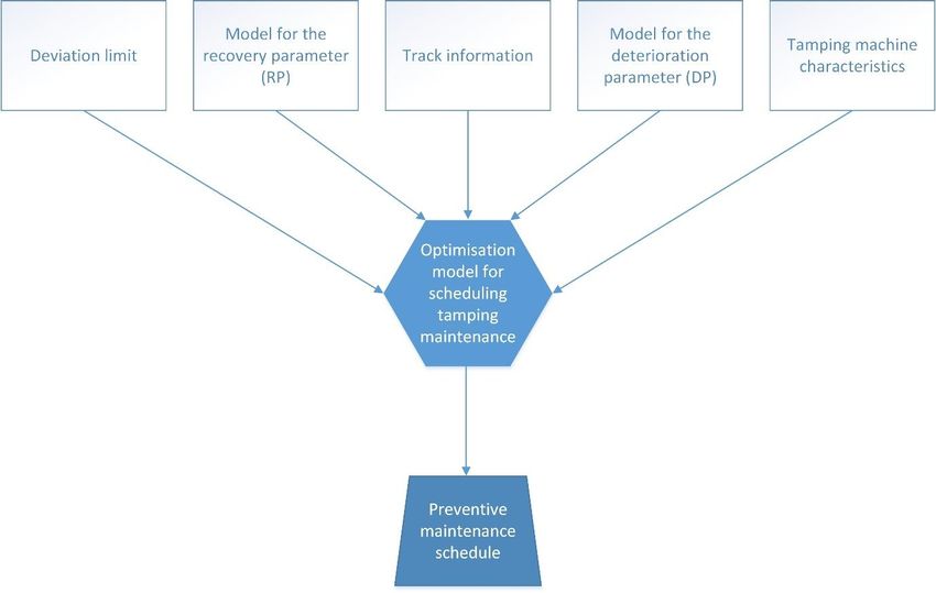
SUMMARY
Scheduling preventive tamping maintenance can be optimised by using optimisation models.
The basis of the optimisation model for scheduling preventive maintenance in this research
consists of a procedure for estimating the track geometry quality. Figure 1 is a simplified
model of the quality development over time. The deterioration parameter (DP) describes how
the quality reduces over time, the recovery parameter (RP) describes how the quality recovers
after maintenance. The optimisation model uses the RP and the DP to make an optimum
schedule and thereby determine when maintenance is needed, which is indicated by the
position of X 1 and X 2 in Figure 1. The quality of the track geometry is inversiley proportional
to the deviation, and should always be lower than the deviation limit.

 Figure 1: General model for estimating the quality of the track geometry.

This research will look at the quality assessment of the track geometry (the basis for RP and
DP in Figure 1), as input for an optimisation model. In most research thus far, only the
standard deviation of the level (σ LL ) has been used to determine the track geometry quality.
The track geometry quality is also dependent on other track geometry parameters. A.R.
Andrade and Teixeira (2014) have discussed in their research that the standard deviation of
the alignment (σ A ) is also important when determining the track geometry quality. In their
paper they have shown that the quality of the track geometry can best be described by
analysing the quality of both the σ LL and the σ A . This leads to the following research question:

 How is the optimisation model for scheduling preventive tamping maintenance
 affected when adding alignment to the track geometry quality assessment?

The answer to this research question is being pursued by answering the following sub-
research questions:

 1. Which optimisation models for scheduling preventive maintenance are leading in
 literature?
 2. How can a current optimisation model for scheduling tamping maintenance
 incorporate a second track geometry parameter as quality constraint?
 3. How can the recovery of the track geometry parameters by maintenance be modelled?
 4. How can the recovery of the track geometry parameters by maintenance be
 determined with data analytics?
 5. By which functions can the deterioration of the track geometry parameters be
 approached?
 6. How can the deterioration of the track geometry parameters be determined with data
 analytics?
 7. Does the incorporation of the alignment as quality constraint lead to a significantly
 different and improved schedule?

ii | Optimisation model for scheduling preventive tamping maintenance

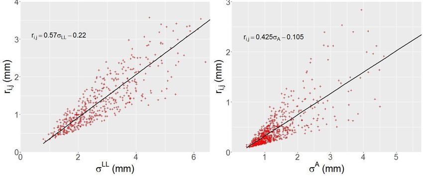
By answering the research question, it will become clear if the optimisation model improves
when adding the alignment in the quality assessment of the track geometry. The sub-research
questions help determining the validity of the used input for the optimisation model.

Research method

The sub-research questions are answered by performing a literature research into
optimisation models for tamping, deterioration methods for the alignment and level, and the
method for determining the recovery parameter. The next step is to build the optimisation
model in CPLEX Studio, and to gather the necessary input information for the optimisation
model. A part of the necessary input information needs to be calculated with the use of data
analytics on historical measurement data. The last step is to simulate the optimisation model
on a test case. The output of the optimisation model which uses only the level will be
compared to the output of the optimisation model which uses both the level and the
alignment to assess the track geometry quality.

Model preparation

The model preparation consists of two elements. The first element is to create two
optimisation models. The first model takes only in account the σ LL , whereas the second
optimisation model uses both the σ LL and the σ A to determine the quality of the track
geometry. The next element is gathering the input data required f or both optimisation
models. The input data consists of the deviation limit, track information, tamping machine
characteristics RP, and DP. The deviation limit is found in the European standard, the track
information and the tamping machine characteristics are supplied by the maintenance
contractor, and the RP and DP needs to be calculated.

The calculation of the RP and DP starts with gathering the raw data and transforming it from
measurement data for every 25 cm of track to the standard deviation of these measurements
over a length of 200 meters. The raw data consist of the measurements for a region of 525
km for the period 2008 to 2013. The next step is to find the trend breaks, which among others
also determine when maintenance is performed. This information is used to determine the
RP, which consists of finding the and of the following equation:

 = ∗ + (1)

The equation states that the total expected recovery ( ) is determined by providing the
quality before maintenance ( ). The constants are calculated by using the aforementioned
data to find all values before and after maintenance to fit a linear correlation between them.
These constants are valid only for the specific region for which they are calculated, since
other regions may have other methods and/or machines. The uncertainty for the calculation
of the RP can be found in Table 1. It shows a high uncertainty for the RP values.

Table 1: Goodness-of-fit for the RP.

 Parameter R-squared RMS 95% interval
 σ LL 0.775 0.400 0.785
 σA 0.634 0.270 0.530

 iii

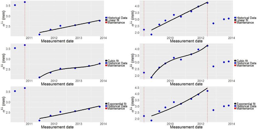
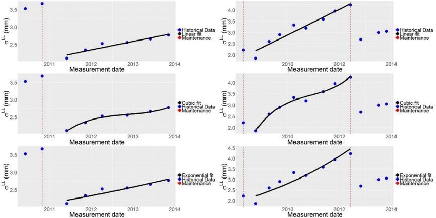
The next step is to find the DP of the σ LL and the σ A , which is often simplified as a function of
time. The functions described in literature are either a linear, cubic, or exponential function.
The fit results for the level and alignment can be found in Table 2. For the σ LL , it is clear that
the exponential function is the best. It has the lowest root-mean-square error (RMS) value,
which means that the range where the actual value lies is relatively small. For the σ A , the RMS
is comparable for all functions, but the linear function has the lowest 95% interval value and
is therefore the best fit. Although the σ LL shows that the exponential function is best, the
optimisation model is currently a mixed integer linear optimisation model. It lies outside the
scope of this research to transform it to a mixed integer non -linear optimisation model.

Table 2: On the left the goodness of fit for the deterioration models for the σ LL , on the right the goodness of fit
 for the deterioration models for the σ A .

 Parameter Function RMS 95% interval

 σLL Linear 0.091 0.178
 Cubic 0.091 0.178
 Exponential 0.058 0.114

 σA Linear 0.056 0.109
 Cubic 0.056 0.111
 Exponential 0.063 0.123

These fits are found by using regression techniques on the measurement data. The
measurement data between two maintenance intervals with at least 5 points are taken into
account or at least 6 measurement points after maintenance are taken into account.

Simulation

The chosen models to calculate the deterioration and recovery are used as input in the
simulation model. The optimisation model makes a binary schedule that determines if
tamping is needed for 10 time periods, where each time period has a duration of 6 months.
The simulation creates a schedule for 5 years with the expected quality evolution of the track
geometry. A schedule is simulated by the optimisation model containing only the σ LL for the
track geometry quality assessment, and by the optimisation model containing both the σ LL
and the σ A for the track geometry quality assessment. Table 3 shows the difference between
the two schedules.

 Table 3: Comparison of the results from the simulations.

 Tamping actions Cost in minutes Machine deployments Simulation time

σ LL 82 1854.8 6 7.93

σ LL + σ A 104 2141.3 6 13.51

Difference 22 (+26.8%) 286.5 (+15.4%) 0 5.58 (+70.4%)

iv | Optimisation model for scheduling preventive tamping maintenance

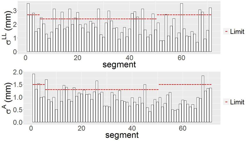
Table 3 shows an increase in the number of scheduled tamping actions. If the σ A is not
included, those extra tamping actions would have led to corrective maintenance. By adding
the σ A to the quality assessment, the optimisation model can use this information to give a
better prediction of the needed maintenance and better cluster tamping maintenance. This
clustering of the tamping maintenance reduces the amount of needed tamping machine
deployments by decreasing the amount of corrective maintenance deployments. The costs
for corrective maintenance deployments is roughly €5000, which means a significant amount
of money can be saved when applying the optimisation model with both σ LL and σ A .

Conclusion

Table 3 has shown that adding the alignment to the track geometry quality assessment le ads
to a different schedule output. The optimisation model σ LL &σ A has significantly more
scheduled tamping actions, which implies that the accuracy is improved by the adjustments,
i.e. the optimisation model is better in determining the evolution of the track geometry
quality over time.

However, the precision of the optimisation model is reduced severely. This means that there
is a high uncertainty when using this optimisation model. The calculation of the recovery
effect by maintenance (RP) has such a broad 95% interval that it is highly uncertain what the
true quality value will be after maintenance. Some track segments need multiple maintenance
actions in the scheduled time horizon, leading to such a high inaccuracy that it is impossible
to know for certain what the added value is of the σ A to the optimisation model. This is caused
by the used data and method in this research to calculate the RP, and not by the equations
to determine the RP.

The addition of the σ A to the quality assessment of the optimisation model for schedule
preventive maintenance leads to a trade-off between accuracy and precision. In this research
the improvements of the accuracy are overshadowed by the decreased precision caused
mainly by the estimation of the RP. When the precision of the RP is improved, the addition of
the σ A increase the insight in the evolution of the track geometry quality, which in turn can
decrease the number of corrective maintenance actions. The optimization model could save
up to €5000 per time period for every prevented corrective maintenance deployment. A
follow-up research with a more precise RP should be conducted to confirm the findings in this
research.

Recommendations

The recommendation for further research consists of adding a more elaborate DP model to
the optimisation model, for example an artificial neural network if possible. It is also
interesting to verify the optimisation model by testing a schedule in practice. Lastly,
considering a time constraint for the maximum allowed time spent during one maintenance
session, should improve the practicality of the optimisation model.

If the optimisation model is used in its current form, it is important to reduce the time horizon
for which the optimisation model makes a schedule. Furthermore, it is important to
recalculate the RP with a much higher precision. The deterioration of the track geometry is
capricious, so although the optimisation model gives more insights in the deterioration of the
track geometry, it can only be used as an aid.

 v

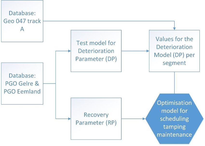
TABLE OF CONTENTS
Preface .............................................................................................................................. i
Summary ........................................................................................................................... ii
List of tables ................................................................................................................... viii
List of Figures .................................................................................................................... ix
1 Introduction of subject ............................................................................................... 1
 1.1 Rail maintenance ................................................................................................. 1
 1.2 Optimisation model for scheduling tamping maintenance ..................................... 2
 1.3 Track geometry parameters ................................................................................. 3
 1.4 Relevance ............................................................................................................ 3
 1.5 Thesis outline ...................................................................................................... 4
2 Research framework ................................................................................................... 5
 2.1 Research questions .............................................................................................. 5
 2.2 Research objective ............................................................................................... 6
 2.3 Limitations .......................................................................................................... 6
3 Research method ........................................................................................................ 7
 3.1 Literature study ................................................................................................... 7
 3.2 Model preparation - Data analytics ....................................................................... 7
 3.3 Simulations - Case study ...................................................................................... 9
 3.4 Thesis structure ................................................................................................. 10
4 Literature Study........................................................................................................ 11
 4.1 Optimisation model ........................................................................................... 11
 4.1.1 Background scheduling preventive tamping maintenance ............................. 11
 4.1.2 Chosen model ............................................................................................. 12
 4.2 Deterioration parameter .................................................................................... 14
 4.2.1 Predicting the quality deterioration of the track geometry ........................... 14
 4.2.2 Calculating the deterioration parameter ...................................................... 15
 4.3 Recovery parameter........................................................................................... 16
 4.3.1 Predicting the quality recovery of track geometry by maintenance ............... 16
 4.3.2 Calculating the recovery parameter ............................................................. 16
5 Model preparation – Data analytics ........................................................................... 18
 5.1 Mathematical equations for the optimisation model ........................................... 18
 5.2 Input parameters ............................................................................................... 21
 5.2.1 Track information ....................................................................................... 21

vi | Optimisation model for scheduling preventive tamping maintenance

5.2.2 Deviation limit ............................................................................................ 22
 5.2.3 Tamping machine information ..................................................................... 22
 5.2.4 Deterioration Parameter & Recovery Parameter .......................................... 23
6 Simulation - Case Study ............................................................................................ 36
 6.1 Optimisation model vs. historical data ................................................................ 36
 6.2 5 year tamping schedule .................................................................................... 37
 6.2.1 Results for optimisation model σ LL ............................................................... 37
 6.2.2 Results for optimisation model σ LL & σ A ....................................................... 38
 6.2.3 Comparison of the results ........................................................................... 39
7 Discussion ................................................................................................................ 41
 7.1 statistical relevance ........................................................................................... 41
 7.1.1 RP model .................................................................................................... 41
 7.1.2 DP model .................................................................................................... 42
 7.2 Assumptions and Decisions ................................................................................ 42
8 Conclusion ............................................................................................................... 44
 8.1 Introduction ...................................................................................................... 44
 8.2 Answer to the sub-research questions ................................................................ 44
 8.3 Answering the main research question ............................................................... 48
9 Recommendations .................................................................................................... 50
 9.1 Recommendation for further research ................................................................ 50
 9.2 recommendations for use of optimisation model ................................................ 50
10 References ............................................................................................................ 52
Appendix I: Measuring track geometry ............................................................................. 54
Appendix II: The standard deviation of the level and alignment ........................................ 55
 Mathematical explanation of the standard deviation ..................................................... 55
 Physical meaning of the standard deviation .................................................................. 55
Appendix III: European norms and the Dutch interpretation ............................................. 57
 European norms and standards .................................................................................... 57
 Netherlands ................................................................................................................. 58
Appendix IV: R-squared and the root-mean-square error of the regression line ................ 61
 R-squared .................................................................................................................... 61
 Root-mean-square error ............................................................................................... 61

 vii

LIST OF TABLES
Table 1: Goodness-of-fit for the RP. ................................................................................................... iii

Table 2: On the left the goodness of fit for the deterioration models for t he σ LL , on the right the
goodness of fit for the deterioration models for the σ A . ..................................................................... iv
Table 3: Comparison of the results from the simulations. ................................................................... iv

Table 4: Raw data specifics .................................................................................................................8

Table 5: European norms for the deviation limits for σ LL and σ A , and the used deviation limits for the
optimisation model (CEN, 2010). ....................................................................................................... 22

Table 6: Tamping characteristics. These characteristics are used as input to determine the total cost
in minutes of the schedule. ............................................................................................................... 23
Table 7: Specifics of the used measurement data. ............................................................................. 24

Table 8: Data characteristics for PGO Gelre and PGO Eemland. ........................................................ 25

Table 9: Data availability of the PGO Gelre and PGO Eemland database. .......................................... 25
Table 10: Data characteristics for database Geo 047. ....................................................................... 27

Table 11: Data availability for the Geo 047 database. ....................................................................... 27

Table 12: Data trends in their meaning. In the data preparation phase, several breaks in trends have
occurred and are described in this table. .......................................................................................... 30

Table 13: Values to find exception 3. ................................................................................................ 31

Table 14: Bounds of the fitted deterioration models. ........................................................................ 32
Table 15: Values to find exception 1 and 3. ....................................................................................... 33

Table 16: The goodness-of-fit of the different functions for the σ LL and σ A . ....................................... 34

Table 17: Comparison between the two optimisation models. ........................................................... 39
Table 18: Goodness of fit for recovery parameter. ............................................................................ 41

Table 19: Goodness of fit for the DP’s for σ LL and σ A . ........................................................................ 42

Table 20: Fit results for the linear regression of the DP. .................................................................... 46
Table 21: The goodness-of-fit of the different functions for the σ LL and σ A . ....................................... 47

Table 22: Comparison of the output of the two optimisation models. ............................................... 48

Table 23: Defects per waveband for level (Esveld, 2015). .................................................................. 54

viii | Optimisation model for scheduling preventive tamping maintenance

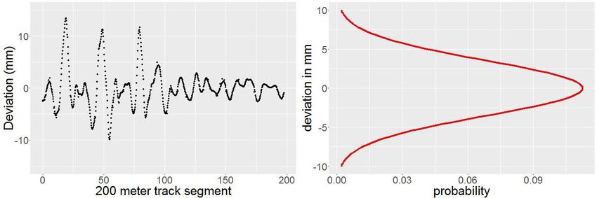
LIST OF FIGURES
Figure 1: General model for estimating the quality of the track geometry. ......................................... ii

Figure 2: Division of the maintenance and renewal activities (Esveld, 2015, p. 387). ..........................2

Figure 3: The right figure shows the principle of an optimisation model, the left figure gives an overview
of the geographical location of segments. ..........................................................................................2

Figure 4: Geometry parameters (Esveld, 2015, p. 16). .........................................................................3

Figure 5: Outline of the thesis. ............................................................................................................4
Figure 6: Location of the acquired data on the left, on the right the location of the case study indicated
as the line with 047. PGO Eemland is the green area, and PGO Gelre is the red area. .........................9

Figure 7: Overview of the chapters.................................................................................................... 10
Figure 8: On the left, example of an analyses of one segment according to the method by Vale et al.
(2012). On the right, the scheduling output for 2 years with 180 segments. ..................................... 12

Figure 9: Block diagram of the optimisation model. .......................................................................... 13
Figure 10: The deterioration of the track geometry (Esveld, 2015, p. 666). ....................................... 14

Figure 11: Calculating the DP for the alignment and the σ LL (Esveld, 2015, p. 590). .......................... 15

Figure 12: Relation between the track geometry quality before maintenance and the expected recovery
(Vale et al., 2012). ............................................................................................................................ 17

Figure 13: Schematisation of the required input information and output of the optimisation model. 18

Figure 14: Tamping in transition curves (Wen et al., 2016). .............................................................. 21
Figure 15: Database information to optimisation model. .................................................................. 24

Figure 16: The distribution of the measurement data for the alignment for the regions PGO Gere and
PGO Eemland. On the left a boxplot, on the right a histogram with the probability density function in
red. ................................................................................................................................................... 26

Figure 17: The distribution of the measurement data for the level for the regions PGO Gere and PGO
Eemland. On the left a boxplot, on the right a histogram with the probability density function in red.
......................................................................................................................................................... 26

Figure 18: The distribution of the measurement data for the alignment of Geo 047 track A. On the left
a boxplot, on the right a histogram with the probability density function in red. .............................. 27
Figure 19: The distribution of the measurement data for the level of Geo 047 track A. On the left a
boxplot, on the right a histogram with the probability density function in red. ................................. 28

Figure 20: Division of the database to workable sizes. ...................................................................... 28
Figure 21: Example of a segment for one time period. A segment has a length of 200 meters, the figure
shows the deviation of the level which will be processed into a single value to assess the quality. The
smaller and less frequent minimum and maximum values, the better the quality. ............................. 29

Figure 22: An example of the trend for a segment. This specific segment has 9 measurement dates,
stretching over 4.5 years. The vertical dashed red line indicate where a trend break occurs. ............ 29

Figure 23: The initial quality of the track per segment. All values should be bel ow the deviation limit,
the red line. The top figure contains the initial quality for the standard deviation of the level (σ LL ). The
bottom figure contains the initial value for the standard deviation of the alignment (σ A ). ................ 30

 ix

Figure 24: Left the recovery effect of maintenance for the σ LL , on the right for the σ A . ..................... 32

Figure 25: Fitted deterioration functions. .......................................................................................... 33

Figure 26: Examples of the two different types of accepted historical data that is used for the DP
analyses. ........................................................................................................................................... 34

Figure 27: Example of the impact of the size of RMS. ........................................................................ 35

Figure 28: Deterioration speed per day in millimetre for every segment. Top plot displays the
deterioration for the σ LL , bottom plot displays the deterioration for the σ A . ...................................... 35

Figure 29: Output of the optimisation model for a single segment. ................................................... 36

Figure 30: Example of the results for one segment for the single parameter optimisation model. ..... 37
Figure 31: Schedule produced by the optimisation model σ LL for 5 years. .......................................... 38

Figure 32: Example of the optimisation model results for two parameters. ....................................... 38

Figure 33: Schedule produced by the optimisation model σ LL & σ A for 5 years. .................................. 39
Figure 34: Example of the importance of adding σ A to the quality assessment. ................................. 40

Figure 35: Example of how the RP 95% interval influences the expected value after maintenance. ... 41

Figure 36: Example of the uncertainty in predicting the quality development by the optimisation model.
......................................................................................................................................................... 42

Figure 37: General model for estimating the quality of the track geometry. ...................................... 44

Figure 38: Results for the linear regression of the DP. ....................................................................... 46

Figure 39: Least square method for fitting the different functions on the historical data. ................. 47

Figure 40: The method for measuring the track geometry parameters (CEN, 2010). .......................... 54

Figure 41: The standard deviation in relation to the percentage of the percentage of data it represents.
......................................................................................................................................................... 55

Figure 42: The measurement data for a single segm ent and year (i) on the left and the normal
distribution of the measured value on the right. ............................................................................... 56

Figure 43: The measurement data for a single segment and year (ii) on the left and the normal
distribution of the measured value on the right. ............................................................................... 56

Figure 44: Comparison of the normal distribution of segment i with segment ii ................................ 56
Figure 45: The data from track geometry data to the vehicle response indicator. ............................. 59

Figure 46: The development of the vehicle effect from data analyses to processing new data. ......... 59

Figure 47: The forces and their direction between wheel and rail. .................................................... 60
Figure 48: Determining the error for a regression line (Freedman et al ., 1998, p. 182). .................... 61

x | Optimisation model for scheduling preventive tamping maintenance

1 INTRODUCTION OF SUBJECT
This research looks into optimisation models for scheduling preventive rail maintenance. This
chapter introduces the subject, with rail maintenance as starting point. The chapter ends with
an outline of the thesis.

1.1 RAIL MAINTENANCE
Railways are an important option for passenger transport and freight transport. In Europe ,
there is an increase in the total amount of passengers and freight moved over rail in recent
years (Eurostat, 2015a, 2015b). It is important to keep the track safe for the users, therefore
railways need maintenance and renewal (M&R). When performing the M&R, the railway track
is unavailable for other traffic. Therefore, a balance must be created for the track possession
between M&R and operations. The ideal situation would be when M&R can be performed
next to operations without negatively influencing each other. The Netherlands has tried to
limit the M&R works to night slots when no or limited rail traffic occurs to approach this ideal.
Those night slots have become shorter in recent years, reducing the available time for
maintenance to less than 4 hours a night. The time during the night slots are too short to
perform all necessary M&R, therefore the M&R works also occur during daytime. This leads
to detours, inaccessible stations, and overall great nuisance for passengers .

Therefore, there is a need for preventive maintenance models that minimize the time spend
on maintenance, while ensuring good infrastructure performance. Preventive maintenance
models can in this way reduce the amount of delays experienced by passengers. Preventive
maintenance models can give indications of the amount of necessary maintenance needed
within a certain time period. These insights can lead to an increased overview of the necessary
maintenance, which enables more flexibility when scheduling. Preventive maintenance
models can also postpone renewals and reduce traffic interruptions, decreasing the time
spent on M&R works. The availability of the track is a very important issue for rail operators.
This has led to performance-based maintenance contracts in the Netherlands, which is a
tender form where the focus lies on minimising the downtime of track lines.

M&R works can be divided according to Figure 2. It shows the actions needed to ensure that
the track meets the safety and quality standards. In the Netherlands the annual activities
regarding R&M for their 4500 km main track consist of renewal of 140 km main track, 40 km
secondary track, 1000 km of mechanical tamping, 60 km of ballast cleaning, 10 km of
corrective grinding, and renewal of 250 switches (Esveld, 2015, pp. 387 - 388). With a work
speed up to 2200 m/h, the Netherlands needs at least 450 hours of mechanized tamping
annually. In practice, tamping machines are used with a far smaller work rate, varying the
amount of time needed for mechanized tamping between 450 and 1000 hours every year.
Since mechanized tamping requires so much resources on an annual basis, models have been
developed to optimise the use of a tamping machine by scheduling preventive maintenance.
The next section will explain the basic principle of optimisation models for scheduling tamping
maintenance.

 Introduction of subject | 1

Figure 2: Division of the maintenance and renewal activities (Esveld, 2015, p. 387).

 1.2 OPTIMISATION MODEL FOR SCHEDULING TAMPING MAINTENANCE
 When scheduling preventive maintenance, it is important to determine how the quality
 develops over time. It is necessary to know when the quality drops to unacceptable levels,
 leading to a need for maintenance. The optimisation models by Li et al. (2015) and Vale,
 Ribeiro, and Calçada (2012) use a deterioration parameter (DP) and recovery parameter (RP)
 to predict how the quality of the track geometry evolves over time. The DP describes how the
 quality decreases over time, while the RP estimates the quality recovery by maintenance. The
 RP is an estimate of the efficiency of maintenance. This is often calculated per country or
 maintenance contractor, since each maintenance provider uses their own machines and
 maintenance procedures. With the use of the RP and DP, the scheduling model can determine
 when maintenance is needed, and schedule it for the lowest possible costs. The costs can be
 squeezed by clustering the maintenance actions.

 The optimisation model analyses the track geometry per segment, which often has a length
 of 100 or 200 meter. The left plot in Figure 3 shows an example of the principle of the
 optimisation model for one segment. The quality of the track geometry can be described as
 the deviation from the design level. When the deviation is 0, the track is in perfect condition;
 when the deviation reaches the limit, maintenance is required or the safety and comfort of
 passengers is not guaranteed. Every country creates their own deviation limit for the track
 geometry derived from international standards. These standards describe how much
 deviation is allowed while still ensuring safety and comfort for passengers.

Figure 3: The right figure shows the principle of an optimisation model, the left figure gives an overview of the
 geographical location of segments.

 2 | Optimisation model for scheduling preventive tamping maintenance

The objective of the optimisation model is to determine what the optimal placement of X is
on the time axis, i.e. it determines the best moment to perform maintenance. The
optimisation model takes into account other segments, which enables it to minimize the times
a tamping machine is needed and thereby reducing the costs of maintenance . The segments
are located next to each other as can been seen in the right picture in Figure 3.

1.3 TRACK GEOMETRY PARAMETERS
Mechanized tamping is used to restore the track geometry quality. A tamping machine lifts
the rails with the fastening and the sleepers from the ballast bed to the desired position and
squeezes the ballast under the sleepers. Mechanized tamping is important since track
geometry determines how the load of the rolling stock (e.g. a train) is distributed on the rails,
and effects the upwards and sideways accelerations of the rolling stock. These accelerations
are important for passenger comfort, and are dependent on the track geometry quality and
speed of the rolling stock. The track geometry parameters consist of gauge, alignment, level,
cant, and twist. Figure 4 shows the graphic presentation of the parameters. Although gauge
is a geometric parameter, it is only partly recovered by mechanized tamping.

 Figure 4: Geometry parameters (Esveld, 2015, p. 16).

When looking at the quality of the track geometry to assess if maintenance by a tamping
machine is required, the quality is often simplified to the standard deviation of the level of
the track (σ LL ). The σ LL is a measure to determine the smoothness of the track over a certain
length. It has been indicated in many research papers as the leading geometric parameter to
determine the quality of the track geometry. However, new research has shown that the
quality of the track geometry is best predicted by looking not only at the σ LL , but also take
into account the standard deviation of the alignment (σ A ) (A.R. Andrade & Teixeira, 2014).

1.4 RELEVANCE
Optimisation models can reduce the amount of disruptions and increase the performance of
the railway. The railway is an important mode of transport for commuting, travelling, and
transporting freight. By enabling lower costs for maintenance and more uptime of the track,
the efficiency of this mode of transportation will go up.

 Introduction of subject | 3

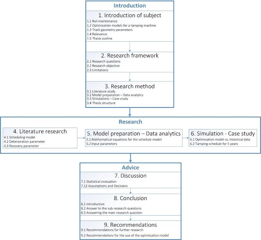
1.5 THESIS OUTLINE
The thesis has 9 chapters, and an overview can be found in Figure 5. Chapter 1 gives an
introduction to the subject. Chapter 2 describes the hypotheses and the research questions.
Chapter 3 describes the method for answering these research ques tions with a link between
the research questions and the different chapters. Chapter 4 presents the literature study,
which includes a background of optimisation models, and the different methods of creating
the input necessary for the optimisation model. Chapter 5 contains the mathematical
equations of the optimisation model and explains which input is necessary for the
optimisation model and how to find them. The outcome will be used in chapter 6 to perform
the simulations on the old and new optimisation model. The output of the old optimisation
model will be compared with the output of the new optimisation model . Chapter 7 discusses
the value of the research by looking at the assumption made and the different statistical
goodness-of-fit values for determining the input parameters. In chapter 8 the conclusion is
presented by answering the research questions. Chapter 9 includes recommendations for the
use of the optimisation model and suggestions for further research.

 Figure 5: Outline of the thesis.

4 | Optimisation model for scheduling preventive tamping maintenance

2 RESEARCH FRAMEWORK
This chapter describes the research framework. In this chapter the research topic will be
explained with the research questions, objective, and limitations.

2.1 RESEARCH QUESTIONS
The research topic consists of altering the process of assessing the quality of the track
geometry as input for the optimisation model to schedule preventive tamping maintenance.
To determine the quality of the track geometry, the standard deviation of the level (σ LL ) and
alignment (σ A ) will be considered. The addition of the σ A to the quality assessment of the
track geometry has consequences for the optimisation model, the Recovery Parameter (RP),
and Deterioration Parameter (DP). The RP and DP are key input for the optimisation model,
which greatly affects the output of the optimisation model. The σ A is assumed to be of
importance for the assessment of the track geometry quality. This leads to the first
hypothesis:

H1: The quality assessment of the track geometry as input for optimisation models can be
improved by taking into account the σ LL and the σ A .

H1 is used to formulate the main research question. The process to assess the quality of the
track geometry is very important as input for the preventive maintenan ce model. Therefore,
the main research question is:

 How is the optimisation model for scheduling preventive tamping maintenance
 affected when adding alignment to the track geometry quality assessment?

There are multiple optimisation models for scheduling preventive tamping maintenance, but
one should be chosen to be used in this research to compare the effect of using σ LL versus
using σ LL and σ A to assess the track geometry quality. The chosen model should be able to
incorporate the σ A next to the σ LL . This leads to the two sub-research questions below.

 1. Which optimisation models for scheduling preventive maintenance are leading in
 literature?
 2. How can a current optimisation model for scheduling tamping maintenance
 incorporate a second track geometry parameter as quality constraint?

The basis for the optimisation model is the quality evolution of the track geometry. The
quality evolution of the track geometry consists of the RP and the DP. The RP needs to be
calculated as input for the optimisation model. The σ LL and σ A are very similar, therefore the
second hypothesis is:

H2: The method to calculate the RP for the σ LL can also be used to calculate the RP for the σ A .

The method for calculating the RP is assumed to be similar for both the σ A and the σ LL . The
process of calculating the RP’s and validating H2 leads to the following sub-research
questions:
 Research framework | 5

3. How can the recovery of the track geometry parameters by maintenance be modelled?
 4. How can the recovery of the track geometry parameters by maintenance be
 determined with data analytics?

Next to the RP, the DP needs to be calculated. In this instance it is important to find a method
for calculating the DP which can be used as input for the optimisation model. Again, it is
assumed that the method for calculating the DP can be similar for both the σ LL and the σ A ,
which leads to the third hypothesis.

H3: The method to calculate the DP for the σ LL can also be used to calculate the DP for the
σA.

When assuming H3 is true, the DP for both the σ LL and the σ A can be calculated in the same
manner. Since the focus of most other research is based on determining the DP of the σ LL ,
these methods need to be verified for the σ A to verify whether and to what extend H3 is true.
This leads to the following sub-research questions:

 5. By which functions can the deterioration of the track geometry parameters be
 approached?
 6. How can the deterioration of the track geometry parameters be determined with data
 analytics?

The schedules from the optimisation model which only uses the σ LL as quality constraint will
be compared with the optimisation model which uses both the σ LL and the σ A as quality
constraint. The answers to research questions 1 to 6 enable the comparison between these
two optimisation models. This leads to the last sub-research question:

 7. Does the incorporation of the alignment as quality constraint lead to a significantly
 different and improved schedule?

H1 is related to the main research objective, whereas H2 and H3 are important to validate
the procedure of obtaining the necessary input required to use the optimisation model for
scheduling tamping maintenance.

2.2 RESEARCH OBJECTIVE
The research objective is to find a better method for determining the track geometry quality,
for the purpose of improving the accuracy of the optimisation model for scheduling tamping
maintenance. This objective has led to the hypothesis that the σ A as addition to the σ LL leads
to a better prediction of the quality development in time. This research goal leads to
investigating the predictability of the DP and RP of the σ A . Research in this area is currently
underdeveloped, meaning that predicting the quality evolution of the alignment over time
needs to be tested in this research as secondary objective.

2.3 LIMITATIONS
There are multiple approaches to predict the DP. In this research only linear and non-linear
models as functions of time are used, whereas neurological network models and other
comprehensive models are not taken into account. The optimisation model will look primarily
at the near future, for which the assumptions made in the optimisation model hold.

6 | Optimisation model for scheduling preventive tamping maintenance

3 RESEARCH METHOD
The research consists of three parts. Simulations will be performed on a case study to find
the effect of adding the standard deviation of the alignment (σ A ) in the quality assessment of
an optimisation model for scheduling preventive tamping maintenance. The case study will
consist of computer simulation where the optimal maintenance schedule will be calculated.
The optimisation model needs information to create the optimum maintenance schedule. The
preparation for the optimisation model consist of editing the model to include the alignment
and gathering other required information. This consist in part of calculating the deterioration
parameter (DP) and recovery parameters (RP) with the help of data analytics. A literature
study will be used to find an appropriate optimisation model and to find methods to perform
the data analytics.

3.1 LITERATURE STUDY
The literature study can be divided into optimisation model, DP, and RP. The literature study
conducted into optimisation models will describe which relevant optimisation models are in
existence. One of those optimisation models will be chosen to use in the case study. An
important demand is the ability of the optimisation model to be able to implement the σ A
next to the σ LL . The optimisation model which only uses the σ LL to determine the quality of
the track geometry will be referred to as “optimisation model σ LL ”, whereas the optimisation
model which determines the quality of the track geometry with both the σ LL and σ A will be
referred to as “optimisation model σ LL & σ A ”. This part of the research will answer research
question 1.

Next, the literature study will look into the RP. The RP can be calculated by different possible
models to estimate how much the track geometry recovers due to maintenance. This chapter
will explain which models are available and which one will be used in the data analytics part
of this research, thereby answering research question 3. The chosen model will be used to
determine how data analytics can calculate the RP.

Lastly, the literature study will look at the DP. The DP is a model on its own to determine how
the quality of a track geometry parameter evolves over time. Chapter 1 has shown a linear
deterioration of the quality as model. The literature study will be used to determine which
other methods are used to model the deterioration of the σ LL and the σ A , thereby answering
research question 5. The different methods will be compared to each other in the data
analytics part of this research, to answer the question if and to what extend the σ LL and the
σ A are predictable. The literature study will also look into how the track geometry quality
measurements can be prepared by data analytics. These methods will be found in the
literature study and executed in the data analytics part of this research. This will partly answer
research question 6.

3.2 MODEL PREPARATION - DATA ANALYTICS
Optimisation model

Data analytics is used to create the necessary input information used by the optimisation
model in the case study. It consist of gathering the raw data, and transforming it to data that
can directly be implemented in the optimisation model. The optimisation model itself needs
to be adjusted so it can use both the σ A and the σ LL . This refers to research question 2.

 Research method | 7

Raw data

The raw data consists of the measurement data for every 25 cm of track, for the track
geometry parameters alignment and level, for several years. The measurement data is given
as the deviation relative to the design value in millimetres. The raw data is collected for two
regions in the Netherlands and a specific track which will be used in the case study. The two
regions are PGO 1 Eemland and PGO Gelre, with a combined track length of 525 kilometres
and 4 to 6 years of historical data. This data is provided by ASSET Rail, the maintenance
contractor of these areas. In Table 4 the specifics of the raw data are given and Figure 6 shows
the location of PGO Gelre and PGO Eemland in the Netherlands. It is noticeable that the data
of Area geo 047 track A consists of either 9 or 11 measurements. This is caused by an
incomplete data set, where for a big part of the track the last two measurements are missing.
The measurement data consists of the level with a wave length of 15 meters and alignment
with a wave length of 9 meters. These wavelengths are chosen from a larger set of
possibilities, but are best applicable to determine the need to use a tamping machi ne. This is
explained in more detail in Appendix I: Measuring track geometry.

Table 4: Raw data specifics

Area Measurement data Time Amount of Kilometre
 period measurements track
 Level 15 meter wavelength
PGO Eemland 2008-2013 12
 Alignment 9 meter wavelength
 525
 Level 15 meter wavelength
PGO Gelre 2010-2013 8
 Alignment 9 meter wavelength
 Level 15 meter wavelength
Geo 047 track A 2010-2015 9 or 11 14.856
 Alignment 9 meter wavelength

1
 PGO stands for “Prestatie Gericht Onderhoud”. Small rail maintenance is subcontracted to
maintenance contractors in the Netherlands. Each region is separately tendered, and is named “PGO
region”. This research uses the raw measurements of regions Gelre and Eemland.

8 | Optimisation model for scheduling preventive tamping maintenance

Figure 6: Location of the acquired data on the left, on the right the location of the case study indicated as the
 line with 047. PGO Eemland is the green area, and PGO Gelre is the red area.

Deterioration parameter

In chapter 1, a linear model was given as an example of a possible quality deterioration model.
By analysing the σ LL and the σ A measurement data over several years for the two regions in
the Netherlands, it can be determined if a linear model may be used to model the
deterioration of the track geometry quality. This analyses will answer research question 5.
The databases of PGO Eemland and PGO Gelre will be used to determine the general method
to model the DP. This method will be used on the smaller dataset, GEO 047 track A, to
determine the DP for the case study.

Recovery parameter

The historical data for the regions PGO Eemland and PGO Gelre will be used to determine
how the RP for the σ LL and the σ A can be calculated. This analyses should give a correlation
between the quality before maintenance and the quality after maintenance. With the help of
the before mentioned literature study, this analyses will give an answer to research questi on
4.

3.3 SIMULATIONS - CASE STUDY
The case study will be performed on geo 047 track A, which location is presented as the grey
line on the right in Figure 6. The simulations are performed by using all the necessary input
information for the optimisation model, which are calculated in the previous research step.
Each simulation will have a tamping maintenance schedule as output. The simulation will be
executed for the same period as the historical data to compare the results of the ac tually
performed maintenance to the scheduled maintenance by the optimisation model. This will
be used as a check to have a rough validation of the optimisation model. The next step is to
make a schedule for 5 years in the future for optimisation model σ LL and for optimisation
model σ LL & σ A . The difference between the outputs of these two optimisation models will be
used to answer research question 7.

 Research method | 9

3.4 THESIS STRUCTURE
The structure of this report can be found in Figure 7 and begins with the
introduction to the subject. The introduction explains the background of
rail maintenance and the reasoning for improving the preventive
maintenance model. The research framework describes the goal,
objective, and research questions for this research. The research method
describes the methods used to answer these research questions and the
data acquired for the case study. The literature study will answer research
question 1, 3, 5, and 6. The literature study contains the bases for the
model preparation chapter. In the model preparation chapter the
mathematical equations for the optimisation model are described and the
different data analyses to obtain the DP and RP are explained. This will
answer research question 2, 4, and 5. The simulation chapter will use all
the relevant information from the previous chapter to perform the
simulations. The simulation of optimisation model σ LL and optimisation
model σ LL & σ A will have different tamping maintenance schedules which
will be compared to each other to answer research question 7. The
discussion chapter will use the information from chapter 4, 5, and 6 to
discuss the validity of the research. The conclusion will give a small recap
of all answers to the research questions and presents the main findings.
The lessons learned during this research and the advice for the usage of
the optimisation model will be presented in the recommendation chapter.
 Figure 7: Overview of the
 chapters.

10 | Optimisation model for scheduling preventive tamping maintenance