Revisiting Telemetry in Pakistan's Indus Basin Irrigation System
←
→
Page content transcription
If your browser does not render page correctly, please read the page content below
water
Article
Revisiting Telemetry in Pakistan’s Indus Basin
Irrigation System
Muhammad Tousif Bhatti *, Arif A. Anwar and Muhammad Azeem Ali Shah
 International Water Management Institute, 12km Multan Road, Chowk Thokar Niaz Baig Road, Lahore 53700,
 Pakistan; a.anwar@cgiar.org (A.A.A.); A.Shah@cgiar.org (M.A.A.S.)
 * Correspondence: Tousif.Bhatti@cgiar.org; Tel.: +92-42-35299504-06; Fax: +92-42-35299508

 Received: 31 July 2019; Accepted: 29 October 2019; Published: 6 November 2019

 Abstract: The Indus Basin Irrigation System (IBIS) lacks a system for measuring canal inflows,
 storages, and outflows that is trusted by all parties, transparent, and accessible. An earlier attempt for
 telemetering flows in the IBIS did not deliver. There is now renewed interest in revisiting telemetry in
 Pakistan’s IBIS at both national and provincial scales. These investments are typically approached
 with an emphasis on hardware procurement contracts. This paper describes the experience from
 field installations of flow measurement instruments and communication technology to make the
 case that canal flows can be measured at high frequency and displayed remotely to the stakeholders
 with minimal loss of data and lag time between measurement and display. The authors advocate
 rolling out the telemetry system across IBIS as a data as a service (DaaS) contract rather than as a
 hardware procurement contract. This research addresses a key issue of how such a DaaS contract can
 assure data quality, which is often a concern with such contracts. The research findings inform future
 telemetry investment decisions in large-scale irrigation systems, particularly the IBIS.

 Keywords: Indus Basin Irrigation System; sensors; telemetry; data contract

1. Introduction
      Pakistan hosts the world’s sixth largest population, estimated at 207.7 million according to the 2017
census [1]. The country consists of four provinces which share water from the Indus Basin Irrigation
System (IBIS). The IBIS is the backbone of Pakistan’s agricultural economy. The agriculture sector,
including crops, livestock, fisheries, and forestry, contributed 18.5 percent to the GDP in 2018–2019 and
is a source of livelihood for 38.5 percent of the nation’s total labor force [2]. The IBIS is a large, complex
system of hydraulic infrastructure that has been developed incrementally over many decades and
represents an estimated US$300 billion in investment [3]. It consists of 2 large reservoirs, 16 barrages,
2 headworks, 12 inter-river canals, and 45 canal irrigation systems, and irrigates an area of the order of
17M ha.
      A formal agreement on the apportioning of the surface water resources of Pakistan between the
four provinces was finally reached in 1991 (herein referred to as the Accord) after long deliberations [4,5].
The Accord, ratified on 21 March 1991, was heralded to remove the biggest hurdle in the way of national
unity and cohesion [5]. Unfortunately, the Accord has been unable to deliver this national unity and
cohesion, which, in turn, has stymied investment and development in water resources. Mistrust
between the provinces and conspiracy theories abound, and at best there is an uneasy peace [4,6].
The lack of trust between the provinces of Pakistan is at the heart of the water issues [7]. The Indus
River System Authority Act 1992 followed shortly after the Accord and paved the way for creating the
Indus River System Authority (IRSA) as stipulated in Clause 13 of the Accord.
      In 2004 the Water and Power Development Authority (WAPDA), a federal government institution
of Pakistan, installed an electronic system to measure depth-of-flow at various key locations along the

Water 2019, 11, 2315; doi:10.3390/w11112315                                        www.mdpi.com/journal/water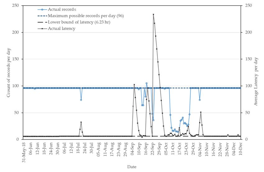
Water 2019, 11, x FOR PEER REVIEW 2 of 19
Water 2019, 11, 2315 2 of 20
In 2004 the Water and Power Development Authority (WAPDA), a federal government
institution of Pakistan, installed an electronic system to measure depth-of-flow at various key
locations
IBIS andalong the IBISthese
to transmit and data
to transmit these data electronically—referred
electronically—referred to as theThe
to as the WAPDA Telemetry. WAPDA
locations
Telemetry. The locations
where WAPDA where
installed WAPDA installed
the telemetry system are theshown
telemetry system
in Figure 1. are
Thisshown
systeminwasFigure 1. This
installed with
system was installed
an investment with an
of US$5.4 investment
million in 2004 of US$5.4
prices [8]. million in 2004 prices
The Government [8]. The
of Pakistan Government
in 2012 of
commissioned
Pakistan
a panelin of
2012 commissioned
international a panel
experts whoofauthored
international experts
a seminal who on
report authored
the watera seminal report
challenges ofon the
Pakistan
water
andchallenges of Pakistan
the way forward. Thisand the way
report, forward.
commonly This report,
known commonly
as the Friends known as the
of Democratic Friends
Pakistan of
(FODP)
Democratic Pakistan
report [6], made the(FODP) report [6],
observation made
that the observation
a decade that a decade
ago, the telemetry system ago,
wastheinstalled
telemetry tosystem
automate
wastheinstalled to automate
measurement the measurement
and reporting process, and
but itreporting process,[6].
has not worked but The
it has not worked
popular [6].Pakistan
press in The
popular press in Pakistan also report that the investment in telemetry has never worked
also report that the investment in telemetry has never worked satisfactorily or been accepted by the satisfactorily
or been accepted in
stakeholders, byparticular,
the stakeholders,
IRSA (e.g.,in particular,
[9,10]). IRSA (e.g., [9,10]).
Figure
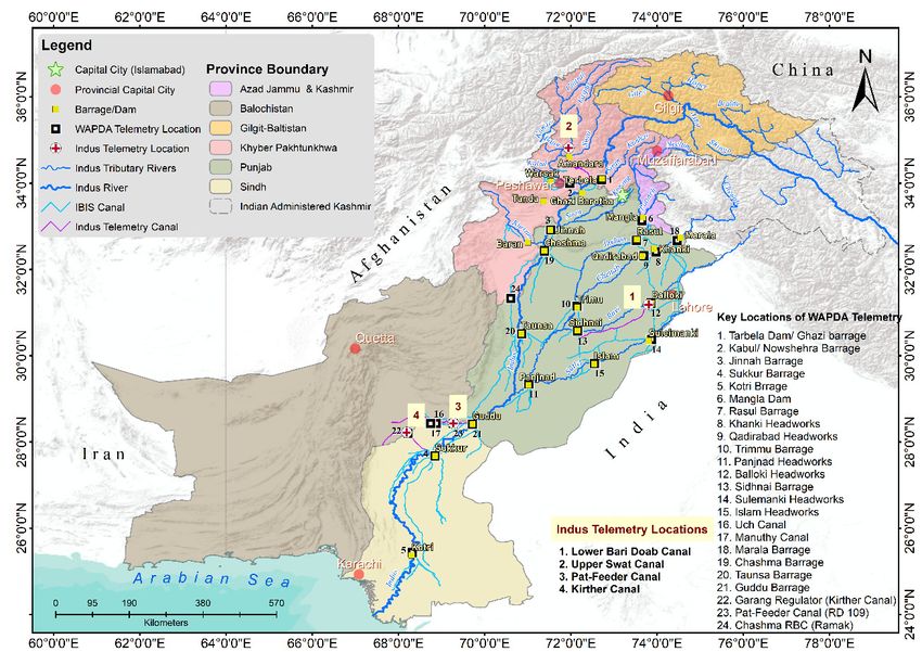
Figure 1. Location
1. Location mapmap of telemetry
of telemetry locations
locations in Indus
in the the Indus Basin
Basin Irrigation
Irrigation System.
System.
Briscoe
Briscoe andand Qamar
Qamar in 2005
in 2005 [11][11] suggested
suggested thethe following
following requirementstotoimplement
requirements implementthe theAccord
Accord in
a transparent manner:
in a transparent manner:
1. “A rigorous, calibrated system for measuring water inflows, storages, and outflows be put in place.
1. “A rigorous, calibrated system for measuring water inflows, storages, and outflows be put in place.
2. The measurement system be audited by a party which is not only scrupulously independent and
2. The measurement system be audited by a party which is not only scrupulously independent and impartial
impartial but is seen to be so by all parties.
but is seen to be so by all parties.
3. Reporting must be totally transparent and available in real time for all parties to scrutinize.”
3. Reporting must be totally transparent and available in real time for all parties to scrutinize.”
This sentiment has been expressed in numerous other reports and studies [12–14]. Importantly,
This sentiment
the Government has been
of Pakistan hasexpressed in numerous
acknowledged the needother
forreports and studies
automated [12–14]. Importantly,
flow monitoring in its
the Government of Pakistan has acknowledged the need for automated
National Water Policy [15], approved in 2018: “Real-time monitoring of river flows by IRSA flow monitoring in its
is National
to be
Water
ensured Policyinter
through [15],alia
approved
telemetric 2018: “Real-time
inmonitoring monitoring
to maintain of river
transparent flowsaccounting
water by IRSA issystem
to be ensured through
and to check
the inter alia telemetric
increasing monitoring to maintain
trend of unaccounted-for water intransparent water accounting
the Indus System of Rivers. system andshould
This task to check
be the increasing
completed
trend of unaccounted-for
before the end 2021”(sic). water in the Indus System of Rivers. This task should be completed before the end
2021”(sic).
Some of the clamor for telemetry in the IBIS stems from the fact that IRSA reports large volume
balance Some
errorsof(referred
the clamor forthe
to in telemetry in the
vernacular asIBIS stems fromevery
losses/gains) the fact that
year. IRSA
The reports
average large volume
(1976–2015)
annual surface water resource of Pakistan is 178.461 Gm /year. The average unaccounted volume annual
balance errors (referred to in the vernacular as losses/gains)
3 every year. The average (1976–2015) for
surface water resource of Pakistan is 178.461 Gm3 /year. The average unaccounted volume for the sameWater 2019, 11, 2315 3 of 20
period remained 22.474 Gm3 /year; hence, approximately 13% of Pakistan’s annual water resource
remains unaccounted-for. During 2014–2015, the unaccounted-for volume reached 36.082 Gm3 /year,
which was more than twice the national reservoir capacity of Pakistan at that time [16]. This inability
to account for water results in recriminations and mistrust between the provinces and in the data and
information reported by IRSA [4,6].
The term “unaccounted-for water” is commonly used for public water utilities performance.
Large amounts of water supplies to major cities remain unaccounted-for, e.g., in Asia, Latin America,
and Africa [17]. In many cases, the data exist with researchers, water users, and local authorities but do
not become available to the water accounting authority. The water accounting in the IBIS is based upon
the system inflows (the aggregated river inflows) and system outflows (aggregated canal withdrawals).
The difference between the system inflows and outflows is referred to as unaccounted-for water or,
more commonly, losses and gains. IRSA receives disaggregated data from various line agencies and
then processes this to prepare national water accounts. The existing data acquisition, archiving, and
reporting system is not robust and the inability to account for potential losses (e.g., evaporation, leaks
from river beds, etc.) gives rise to unaccounted volumes. Principle #5 of the Organisation for Economic
Co-operation and Development (OECD) Principles on Water Governance states, “Produce, update, and
share timely, consistent, comparable and policy-relevant water and water-related data and information, and use
it to guide, assess and improve water policy.” [18,19].
The Government of Pakistan has re-engaged with the issue of water data and information in the
recent years. The Government is undertaking a project (World Bank Project identifier P110099; closing
date 30 June 2021) that includes an activity for “automation of flow measurement and information
system for the IBIS using telemetry system and modern techniques” with the objective that this will
scale up efforts to increase transparency in the inter-provincial water allocation system and contribute
to water conveyance efficiency in the IBIS [20]. Similarly, the provincial Governments have also
invested [21,22] in the installation of hydro-met and real-time flow monitoring.
This paper presents the experience of a pilot study instrumenting canals in the IBIS (herein called
the Indus Telemetry) to demonstrate technological choices and, more importantly, how the quality of
acquired data can be ensured, particularly when data are supplied as a service. A Data as a Service
(DaaS) contract in the water sector, as opposed to more conventional hardware procurement contracts,
requires more careful consideration of the data quality. This research offers insight into a data quality
process by expanding on its various steps and assesses its attributes or dimensions such as integrity,
timeliness, and accuracy. The authors develop and apply a new statistical indicator for data timeliness
and also analyze data integrity and accuracy by using appropriate statistical indicators. This research
also addresses the question of what should be the statistical limits (upper or lower bounds) for the
indicators used to assess data quality. Previous work on this topic is limited; therefore, the present
research will lead to new knowledge in the quality assurance of water data and information that,
in turn, will foster trust and confidence in the data acquired.
2. Materials and Methods
2.1. The Study Area
Figure 1 shows a map of the Indus Basin Irrigation System (IBIS) indicating the four pilot locations.
The figure also identifies 24 key locations where the Water and Power Development Authority (WAPDA)
set up a telemetry system in 2004. Notably, many of these key locations are barrages where more than
one canal take off from the river. Thus, WAPDA installed at these key locations multiple water level
sensors (non-contact ultrasonic range finders): at the rivers, upstream and downstream of the barrage,
and at canals, downstream of the head regulator. In addition to the water level sensors, WAPDA also
installed sensors to monitor gate openings of the barrages and regulators.
To estimate discharge in open channel flow (rivers and canals), there is a wide range of techniques
and instruments to choose from. Jamitco et al. [23] described a system that detects water elevationWater 2019, 11, 2315 4 of 20
using an ultrasonic range finder. The data from the range finder can be used to estimate depth-of-flow
in the channel, and using a rating curve the velocity and discharge can be estimated. More recently,
there has been considerable interest and development in acoustic Doppler current profilers (ADCP) [24]
that can estimate velocity directly and avoid the need/use of velocity rating curves. A number of
authors, e.g., [25–27], among others, have compared the velocity estimates from ADCPs with more
conventional mechanical or electromagnetic current meters and found good agreement.
For automatic data acquisition in the present study (i.e., Indus Telemetry), we selected one main
canal from each of four provinces of Pakistan. This selection scheme was deliberate to ensure coverage
in all provinces, and the particular canal (and the specific location on each canal) was selected on the
advice of the respective provincial irrigation department to ascertain their ownership in the instruments
and data. The selected canals originate from three rivers—the Ravi, Swat, and Indus rivers—and
irrigate around 1.1 Mha of agricultural land (Table 1). Among the four selected canals, Pat Feeder and
Kirther are inter-provincial canals which originate from the Indus River at the Guddu and Sukkur
barrages, respectively, in the Sindh province, but supply in the downstream reaches around 72% of
Balochistans annual water share (4.774 Gm3 /year). The Lower Bari Doab Canal is a large canal selected
in Punjab. This canal irrigates 0.688 Mha of land in Punjab. The Upper Swat Canal was selected in
Khyber Pakhtunkhwa province. It originates at the Amandara headworks on River Swat and diverts
68 m3 /s to irrigate over 107,647 ha of land in addition to supplying water for hydropower generation.
Table 1. Selected canals for Indus Telemetry.
Lower Bari
Feature Unit Upper Swat Canal Kirther Canal Pat Feeder Canal
Doab Canal
River (Barrage/Headworks) Ravi (Balloki) Swat (Amandara) Indus (Sukkur) Indus (Guddu)
Running distance km 8.99 5.94 35.35 33.22
Discharge Estimation Flume Crump Weir Rating Curve Rating Curve
m3 s−1 263.12 101.94 67.96 189.72
Capacity at head
ft3 s−1 (9292) (3600) (2400) (6700)
Khyber
Geographic coverage Province(s) Punjab Sindh-Balochistan Sindh-Balochistan
Pakhtunkhwa
Proportion of total
% 8.8 27.7 22.1 * 49.7 *
provincial water share
Length (km) 201 129 84 171
Irrigated area (ha) 687,967 111,740 107,647 205,753
* Percent share of Balochistan province only.
The instruments were not installed immediately downstream of canal head regulators.
High turbulence and surface waves cause fluctuating readings at such locations. Stilling wells
provide a partial solution to this problem by making gauge reading quiescent. However, measuring
velocity and discharge in highly turbulent water still remains a challenge, and developing a function
between depth-of-flow and discharge—the rating curve—becomes difficult. The instruments were
installed at the locations where the provincial irrigation agency reports discharge, i.e., either at the
discharge measuring structures (e.g., flume or weir) or a canal cross section where a depth–discharge
function (or rating curve) is already available. Pat Feeder and Kirther are inter-provincial canals, and
there are no discharge measuring structures at these locations. At these two canals, rating curves are
used to estimate discharge from depth-of-flow, but the provincial irrigation agencies do not always
agree on the rating curves and the consequent discharge estimates. Table 1 also shows the running
distances along the canals where ultrasonic sensors were installed. The instruments were commissioned
at these four locations during the second and third quarters of 2018. The data were acquired regularly
at 15 min intervals since then. We analyze varying lengths of time series data in subsequent sections of
this paper.
2.2. The Instruments and Data
Five ultrasonic sensors with ancillary components (data loggers, power supply, and modem)
similar to those described by [23] were installed at selected locations of the four canals to measureWater 2019, 11, 2315 5 of 20
depth-of-flow in these canals. The Upper Swat Canal splits into two channels at the measurement
location; thus, two ultrasonic sensors were installed on this canal. The list of main instruments used
in this work is provided in Table A1 (Appendix A). Data were transmitted using General Packet
Radio Services (GPRS) technology to a cloud server (Microsoft Azure Data Centre) where they were
processed, archived, and disseminated to users.
2.2.1. Data Sampling Period
The data sampling period is the time between samples (measurements). Typically, the data
sampling periods can be small, i.e., samples can be taken at high frequency, but the data sampling
period may depend on the “warm-up” time of instruments, i.e., some instruments do require a voltage
to be applied for a short duration first to allow the circuits to reach normal operating temperatures.
2.2.2. Data Logging Period
The data logging period is the time period at which data is logged (recorded) at the data logger.
Data logging is done typically at a higher period—lower frequency—than sampling. Therefore, some
aggregate function, i.e., average, sum, maximum, minimum, is applied to the sampled data which are
then logged in the data logger. The logged data are also date–time stamped. It is important to note
that the date–time stamp is that at which data are logged, rather than that at which they are sampled;
therefore, the data must be interpreted accordingly. Data loggers do not normally store any record of
the sampled data after they are aggregated.
2.2.3. Data Transmission Period
The data transmission period defines the period at which data that have been logged are
transmitted, and this is typically multiples (including one) of the data logging period. In this work,
data were transmitted using a modem, cellular phone network, and GPRS technology. The instrument
was powered by a modest solar panel (20 W capacity) and a rechargeable battery.
2.3. Calibration and External Parameters
The ultrasonic sensor measures the range from the sensor face to the water surface. These raw data
are logged and transmitted to the server where they are post-processed to obtain depth-of-flow. This
post-processing requires the instrument elevation and canal bed elevation. The practice to estimate
discharge in the IBIS is to assume that the canals behave as wide rectangular channels under uniform
flow, and hence, the discharge rating curve is of the form
Q = CH5/3 (1)
where Q is the discharge; C is the rating curve coefficient determined empirically; and H is the
depth-of-flow. From L’Hôpital’s Rule and the Manning equation, the coefficient in Equation (1) is
given by
BS1/2
C= (2)
nr
where B is the width of the canal; S is the bed slope of the canal; and nr is the Manning roughness
coefficient. Equation (1) is often generalized to
Q = CHm (3)
where the coefficient C and m in Equation (3) are determined from flow meter measurements and an
ordinary least squares linear regression of a log transformation of Equation (3).Water 2019, 11, 2315 6 of 20
2.4. Data Post-Processing Delay
In this work, once the sampled average range was received at the server, the depth-of-flow and
discharge were estimated. However, to avoid what is known in computing as a “race condition”
wherein data are being transmitted and processed at the same time (a race between two processes which
may lead to instability), a post-processing delay was introduced to allow the data to be transmitted
first and then to be post-processed.
2.5. Quality Assurance of Data
A six-step data quality process was suggested by [28] based on best practices from data quality
experts. The six steps are definition, assessment, analysis, control, implementation, and improvement.
This research adopted the data quality process by [28] and expanded on the first two steps, i.e.,
the definition step and assessment step, in relation to data from Indus Telemetry.
The definition step sets up the foundation of the data quality process. It includes clarifying what
are the business goals, roles, and responsibilities of the parties and data rules in a DaaS contract.
Clear, specific, and well-documented definitions enable smooth implementation of DaaS contracts.
For example, the goal of Indus Telemetry is to make canal flow data available to the data owner.
In Pakistan, the Indus River System Authority (IRSA) is potentially the owner of the flow data. IRSA
would be the client awarding the DaaS contract to the contractor. The contractor would be responsible
for supplying quality-assured data to the client that comply with the agreed data rules.
The data rules are the essential conditions which data should fulfill to pass the data quality
process, e.g., frequency, data integrity, lower bounds of latency, etc. Moreover, the data rules would also
feature which statistical tests should be used to check data accuracy and what will be the lower/upper
bounds of these statistical tests. We explain the features of data rules in this section and discuss their
application (i.e., assessment step) in Section 3.
The second step of the data quality process is the “assessment step” where acquired data are
assessed in accordance with the defined data rules in the first step. The assessment covers multiple
dimensions of data quality such as its integrity, timeliness, accuracy, etc. To assess data integrity
and accuracy, we considered various statistical indicators as explained in the subsequent subsections.
The application and appropriateness of these statistical indicators are discussed in Section 3. We also
developed a new statistical indicator to assess data timeliness.
2.5.1. Data Integrity
Data integrity in the context of the DaaS contract explains how complete the data are when
compared with the agreed frequencies defined in the definition step. Data integrity is calculated as
shown in Equation (4) and expressed as a percentage. The DaaS contract could specify an upper bound
for data integrity below which the DaaS contractor may incur a penalty. In this research, the sensor
data were logged every 15 min; hence, the maximum possible number of records per day was 96.
count o f data records recieved during a time interval
Data Integrity = × 100 (4)
max. possible data records during a time interval
2.5.2. Data Accuracy
Inaccuracies in electronic data (flow data) may arise due to any one or combination of the following
reasons: poor calibration of a sensor; the use of inaccurate parameters in programming the sensor or
data logger; the post-processing of raw data into information. When such inaccurate data are presented
to the users, it invites critique of the electronic data acquisition methods. This is exactly what happened
in the past when WAPDA installed a telemetry system in Pakistan. When the telemetry data were
compared with the manual data, they did not match, which raised questions about the accuracy of the
electronic data and hampered the ownership of the telemetry system [29,30]. The assessment of data
accuracy is therefore very important to develop confidence in electronic data collection techniques.Water 2019, 11, 2315 7 of 20
Conducting an accuracy assessment for any data requires an agreed-upon reference dataset with
a high level of accuracy [31]. In this case, it is not clear which of the two sensors has superior accuracy.
Therefore, we present our results as a comparison of the level of agreement between the data from the
two independent sensors, i.e., ultrasonic sensor and pressure transducer.
The dataset used in the accuracy assessment is depth-of-flow collected with an ultrasonic sensor
and pressure transducer. For this we installed pressure transducers in addition to the ultrasonic sensors
at the measurement location. Pressure transducers measure liquid levels through a sensor submerged
at a fixed level under the water surface. We applied various statistical tests to assess the data accuracy.
In the interest of brevity, we present an assessment of the accuracy of data from only one canal (Lower
Bari Doab Canal), comparing data from the two independent sensors.
(i) t-test
To assess the accuracy of data, we first need to decide whether the data are for a sample or a
population. In this case, for each measurement with an ultrasonic sensor we also have the corresponding
check measurement with a pressure transducer, and the variable of interest is the difference between
the measurement and the check measurement. Therefore, we have data for the entire population of
measurements. This implies we are estimating population parameters rather than sample statistics,
i.e., population mean, population standard deviation, etc., and not sample mean, sample standard
deviation, etc.
Inferential statistics [32] uses a random sample of data taken from a population to describe and
make inferences about the whole population. This is valuable when it is not possible to examine each
member of an entire population. Student’s t-test is a commonly used inferential statistical method for
hypothesis testing about the mean of a small sample drawn from a normally distributed population.
Similarly, the paired t-test is applied to statistically determine whether the mean responses are the same.
In a particular time period of interest, the count of measurements from both sensors was identical,
which depends on the frequency at which the sensors were programmed to log the data (i.e., 15 min).
As we were considering all the measurements from both sensors, the data constitute the population
rather than a randomly drawn sample.
Since we already know the population mean, we do not need to try to draw inferences (test
hypothesis) about the population mean from the sample mean. Furthermore, the aim of comparing the
two data sets here is to check the data accuracy and not to draw conclusions about some unknown
aspect of a population based on a random sample. Hence, the t-test (or other inferential statistics) is
not an appropriate method to assess data accuracy; rather, descriptive statistics should be applied.
(ii) Difference Plot and Normality
Borrowing from their wider applications in the medical field, difference plots were used in this
work to compare the two methods of measurement, i.e., the ultrasonic sensor and pressure transducer.
The detailed procedure of difference plots was first suggested by Bland and Altman [33] in 1986.
Bland and Altman, in their publications [34,35], explained in detail their method and also provided
a non-parametric approach which is particularly useful in cases when the difference between the
methods does not have a normal distribution. The non-parametric approach is similar to the basic
approach of the difference plot as explained in [34,35] up to and including the plot of the differences
versus the mean values of the two methods. There are then two similar ways of describing such data
without assuming a normal distribution of differences. We can calculate the proportion of differences
greater than some reference value (such as 3 cm in this case). The reference value can be indicated
on the scatter diagram showing the differences versus the mean. Alternatively, we can calculate the
values outside which a certain proportion (say 10%) of the observations fall. To do this we order the
observations and take the range of values remaining after 5% of the observations are removed from
each tail. The centiles can then be superimposed on the scatter diagram. In a DaaS contract, we suggestWater 2019, 11, 2315 8 of 20
that when a non-parametric approach to the difference plot is used, the reference values should be
agreed upon by the client and contractor and defined at the definition step.
Bland and Altman also showed in [35] how a grade can be assigned to a method (sensor in our
case) based on the proportion of observations in a predefined range of the reference values. In this
paper, we developed a criterion and applied it to grade our sensors. Bland and Altman commented
that the “nonparametric method is disarmingly simple yet provides readily interpreted results. Perhaps its
simplicity has led to the belief that it is not a proper analysis of the data”.
Bland and Altman responded to the critique on their proposed method in their 2003 publication [31]
and concluded,
“ . . . It (difference plot) can be extended to many more complex situations, when distributions are not
normal, when difference is related to magnitude, when there are repeated measurements on the same subject,
either paired or not, and when there are varying numbers of observations on subjects”.
It was further stressed in [36] that agreement is a question of estimation, not hypothesis testing.
Estimates are usually made with some sampling error, and limits of agreement are no exception.
The common goal usually is to decide whether a new measurement system agrees suitably
with an existing one and, hence, whether the two can be used interchangeably [37]. The goal of a
comparison of two methods may vary in emphasis by context, as explained by [38], who highlighted
four possible goals:
i. Calibration problems, which deal with establishing a relationship between a new system and
an existing one that can be used to appropriately adjust the new system’s measurements;
ii. Comparison problems, which deal with assessing the level of agreement between two
measurement systems whose measurements are on the same scale;
iii. Conversion problems, which deal with the comparison of two systems whose measurements
are on different scales; and
iv. Gold-standard comparison problems, which deal with the comparison of a new measurement
system with a system that is known to make measurements without error.
The “comparison problem” best defines the goal of comparing two methods of measurement
(sensors) in our case, for which we plot and discuss difference plots using the parametric and
non-parametric approaches.
(iii) Mean Absolute Percentage Error (MAPE) and Symmetric MAPE (sMAPE)
We also apply statistical tests to estimate the error in the depth-of-flow data collected with the two
independent sensors. The mean absolute percentage error (MAPE) is a relative measure that expresses
errors as a percentage of the actual data, as shown in Equation (5). Its advantage is that it provides an
easy and intuitive way of judging the extent or importance of errors.
P
100 xi − yi
Mean Absolute Percentage Error (MAPE) = (5)
n xi
Here, xi are the actual data, yi are the forecasted or estimated data, and n is the number of
non-missing data points.
However, [39] noted that the formula for the MAPE is not symmetric in the sense that interchanging
xi and yi does not lead to the same answer, despite the fact that the absolute error is the same before
and after the switch. The cause of this asymmetry lies in the denominator of the formula—dividing by
yi instead of the actual xi leads to a different result.
This issue has been discussed by many researchers ([40,41], among others), with [41] proposing a
variation of the MAPE formula to provide symmetry: this is known as the sMAPE (symmetric meanWater 2019, 11, 2315 9 of 20
absolute percentage error) and was originally introduced by [42]. The formula suggested by [42] and
the later modification by [43] are given in Equations (6) and (7):
1 xi − yi
sMAPEArmstrong × 100 (6)
n (xi + yi ) ∗ 0.5
1 yi − xi
sMAPEFlores = × 100. (7)
n yi + xi
A limitation of sMAPE is that if xi or yi is zero, the value of the error will be equal to the upper
limit of the error, i.e., 200% for the Armstrong formula and 100% for the Flores formula.
2.5.3. Measurement of External Parameters
Obtaining useful information from telemetry data requires external parameters for processing.
The external parameters include the information that is not or cannot easily be measured through
instrumentation and telemetry. In the case of flow measurement in the IBIS using ultrasonic sensors,
the critical parameters are the bed elevation and the rating curve coefficient in Equation (3). We measured
these two critical parameters for 17 tertiary canals of a typical canal system in the Punjab province
(i.e., the Hakra Branch Canal system, described in detail in [44–46]). The measurements included a
baseline survey of all the canals (at a cross section near a head regulator) in the year 2014 and four
subsequent surveys over the year of 2015. An acoustic Doppler current profiler (ADCP) was used to
measure discharge during the surveys. The variations in the bed elevation and rating coefficient were
then calculated as percent changes from the baseline.
3. Results and Discussion
In this work, the range to the water surface was sampled (measured) every 60 seconds. The data
logging period was set to 15 min, and averaging was used as the aggregate function. Hence, the data
logger logged the average water surface elevation for the 15 min preceding the date–time stamp.
Data transmission from all canal locations was scheduled three times each day at 0745, 1145,
and 1545, Pakistan Standard Time. This means that all transmissions were made during daylight
hours, and the datalogger was programmed such that the system does not attempt to transmit data if
the battery voltage is below a threshold value (in this case set at 11 V). Further, if the battery voltage
falls below a critical value (i.e., 9 V) the sensor stops recording data. Although it is tempting to
transmit data frequently, data transmission is the most power-consuming process of an automated
data acquisition system. This is not an issue during daylight hours when the solar panels can generate
power, but excessively frequent data transmission can drain the battery and lead to system shut-down
at night-time or during overcast winter days with shorter day lengths. A post-processing delay of
10 min was used in this work.
The sampling period was set through appropriate programming of the data logger which excites
the sensor—in this work, 1 min. Sampled data points are only stored temporarily in a data logger
until an aggregate function is applied to the sampled data. In a DaaS contract, it would be difficult to
specify or validate/verify sampled data. However, when the aggregate function is applied to the data,
a count of the sample size that is aggregated can be recorded. Sample size is given by
TD
NS = (8)
TS
where NS is the sample size aggregated at the data logging period; TD is the data logging period; and
TS is the data sampling period. Hence, Equation (8) provides the maximum or upper bound on the
sample size that is aggregated. The actual sample size may be less than this due to hardware/software
failures. Hence, a DaaS contract could specify a threshold value, and a contractor in response couldWater 2019, 11, 2315 10 of 20
adjust the data logging period and data sampling period to exceed the threshold value while allowing
for occasional hardware/software failures. For the parameters used in this work, the sample size
was 15.
3.1. Data Integrity
Table 2 shows the data integrity for all four canals during the reporting period. The table shows
that data integrity was more than 90 percent in all cases. The Pat Feeder and Kirther canals showed
the highest data integrity of above 99 percent. A low value of data integrity indicates that the data
from the sensor were not recorded in the data logger. Other than physical damage to the system
and/or components, this normally happens due to manual power shut down for troubleshooting or
low voltage at the sensor/data logger. In our experience, during long spells of rain, overcast, or fog,
the solar panels do not supply enough energy to charge the battery and the system shuts down if the
battery voltage drops below 9 V.
Table 2. Data integrity and timeliness.
Canals Lower Bari Doab Canal Kirther Canal Pat Feeder Canal Upper Swat Canal
Reporting period during 2018 31 May to 10 Dec 15 Aug to 10 Dec 07 Sept to 10 Dec 09 July to 10 Dec
Average Latency per day hr 17.10 13.33 8.09 8.37
Data records received # 17,057 11,296 8818 29,281
Max possible records # 18,528 11,328 8832 29,952
Data Integrity % 92.1 99.7 99.8 97.8
Note: Lower bound of latency with current transmission frequency is 6.21 h.
3.2. Data Timeliness
Latency is defined as the time that elapses between when a sample is taken and when those data
and derived information from post-processing are accessible to a user. However as defined earlier,
the sampled data are not retained in the data logger; rather, only an aggregation is applied to the
sample. Furthermore, the date–time stamp is that at which the aggregate function is applied rather
than the date–time at which it is sampled. Hence in this work, latency is the time that elapses from
when the aggregate function is applied to when the data and derived information become accessible
to a user. Latency is a function of the data logging period, data transmission period, and data post
processing delay and is given by
T
P TDT −1
(∆ + iTD )
L = i=1 T (9)
T
TD
where L is the latency; TT is the data transmission period; i is an index (0,1,2, . . . ); and ∆ is the data
processing delay. The data transmission period is expressed as any multiple (including one) of the data
logging period. The expression in Equation (9) determines the lower bound of latency. The observed
latency will be equal to or higher than this lower bound if there are hardware or software failures.
For the parameters selected in this work, the lower bound of the latency was 6.21 h.
Table 2 shows the observed latency of the data from all four canals during the specified reporting
period. The data from Lower Bari Doab Canal had the highest average latency per day (17.10 h) followed
by Kirther Canal (13.33 h). Data from Pat Feeder and Upper Swat Canals showed slightly higher
latency than the lower bound of latency (6.21 h). High latency values indicate delays in transmission
that are due to any number of reasons, including but not limited to poor Internet connectivity and
inadequate power to start up the modem.
Figure 2 provides some further insight into the data integrity and latency for the Lower Bari
Doab Canal. The figure presents a daily count of records and latency for the reporting period. The
upper bound of the record count per day was 96 (as explained in Section 2.5.1) and the lower bound
of latency was 6.21 h. Ideally the record count per day should be 96, but if data are lost, the recordWater 2019, 11, 2315 11 of 20
count falls below 96 and, hence, data integrity decreases. Similarly, if the data are received without any
failure, the latency will be identical to the lower bound of 6.21 h, but where there are transmission
failure(s), the latency increases above 6.21 h. Figure 2 shows that data integrity and latency were not
Water 2019, 11, x FOR PEER
interdependent uponREVIEW
each other. 11 of 19
Figure
Figure 2. Observed
2. Observed datadata records
records andand latency
latency perper
dayday
for for
the the Lower
Lower BariBari
DoabDoab Canal.
Canal.
In Figure 2, a high fluctuation is observed in the latency (black continuous line), but the record
This discussion on latency leads into the broader question of what constitutes “real-time” flow
count (blue continuous line) remained relatively stable over the period 4 September 2018 to 8 October
data, as advocated by Briscoe and Qamar [11]. One interpretation of real time is zero latency, which
2018. The high fluctuation in latency is primarily due to poor Internet connectivity in the area where
would be near impossible, expensive to achieve, and probably unnecessary. It would be more realistic
instruments were installed. The system experienced power issues from 9 to 27 October 2018, and
to specify quasi-real-time flow data by specifying the latency in a data as a service (DaaS) contract. A
hence there was a substantial decrease in the record count (data loss) during this period. Interestingly,
pragmatic approach can be to specify separate day-time and night-time latency. Hence, a DaaS
the Internet connectivity improved in this period, resulting in an improvement in the latency. A couple
contract could specify an upper bound on latency (the lower bound is a value calculated by using
of instances of high latency were observed during November and December but with no drop in the
Equation (9)). By way of example, if an upper bound of 12 hours is specified, then latency must not
record count. This occurred due to occasional network failure at the time of transmission. It can be
exceed 12 hours or this will incur a penalty. The configuration as shown in Figure 2 does not fulfil
inferred from Figure 2 that the average latency and record count were not inversely proportional but
the terms of this specification for 15 percent of the time, which would incur the penalty and encourage
rather behaved independently.
the DaaS contractor to find a solution to this problem. Again, a DaaS contract would specify the
This discussion on latency leads into the broader question of what constitutes “real-time” flow
record count, and it would be up to the contractor to program a data logger to ensure that the actual
data, as advocated by Briscoe and Qamar [11]. One interpretation of real time is zero latency, which
record count equals or exceeds the specified threshold.
would be near impossible, expensive to achieve, and probably unnecessary. It would be more realistic
3.3.toData
specify quasi-real-time flow data by specifying the latency in a data as a service (DaaS) contract.
Accuracy
A pragmatic approach can be to specify separate day-time and night-time latency. Hence, a DaaS
To analyze
contract couldthe accuracy
specify of data,
an upper we analyzed
bound the(the
on latency depth-of-flow
lower bound in the
is aLower Bari Doab by
value calculated Canal
using
measured
Equation with
(9)).anByultrasonic sensor and
way of example, if anpressure transducer
upper bound at 15 min
of 12 hours frequency.
is specified, thenNormality testsnot
latency must
were applied
exceed to the
12 hours ordifference between
this will incur the measurements
a penalty. (d-b-m).
The configuration While
as shown plotting
in Figure the difference
2 does not fulfil the
plots, limits of agreement (LoAs) were calculated using the mean and standard deviation
terms of this specification for 15 percent of the time, which would incur the penalty and encourage when thethe
data followed
DaaS a normal
contractor to finddistribution.
a solution to Ifthis
this was notAgain,
problem. the case,
a DaaSa non-parametric versionthe
contract would specify of record
the
difference plot was used to calculate the limits. Table 3 shows the results of various normality
count, and it would be up to the contractor to program a data logger to ensure that the actual record tests
applied
counton the d-b-m.
equals The results
or exceeds suggest
the specified that the data were not normally distributed.
threshold.
Table 3. Normality tests applied to differences between depth-of-flow measured by ultrasonic sensor
and pressure transducer (June 2019).
Normality Test N α t-stat t-crit p-value Decision Rule
t-stat > t-crit p-value < α
Kolmogorov–Smirnov 2817 0.05 0.5139 0.0256 Reject HoWater 2019, 11, 2315 12 of 20
3.3. Data Accuracy
To analyze the accuracy of data, we analyzed the depth-of-flow in the Lower Bari Doab Canal
measured with an ultrasonic sensor and pressure transducer at 15 min frequency. Normality tests were
applied to the difference between the measurements (d-b-m). While plotting the difference plots, limits
of agreement (LoAs) were calculated using the mean and standard deviation when the data followed a
normal distribution. If this was not the case, a non-parametric version of the difference plot was used
to calculate the limits. Table 3 shows the results of various normality tests applied on the d-b-m. The
results suggest that the data were not normally distributed.
Table 3. Normality tests applied to differences between depth-of-flow measured by ultrasonic sensor
and pressure transducer (June 2019).
Normality Test N α t-stat t-crit p-value Decision Rule
t-stat > t-crit p-value < α
Kolmogorov–Smirnov 2817 0.05 0.5139 0.0256 Reject Ho
Anderson–Darling 2817 0.05 6.3903 0.7518 0.0000 Reject Ho Reject Ho
Jacque–Bera 2817 0.05 22.9684 5.9915 0.0000 Reject Ho Reject Ho
Cramer–von Mises 2817 0.05 4.5720 0.2200 Reject Ho
Null Hypothesis Ho = Depth-of-flow is normally distributed; Alternative Hypothesis Ha = Depth-of-flow is not
normally distributed.
Figure 3a presents the depth-of-flow measured using the two sensors with a line of equality.
The correlation coefficient is weak between the data (r2 = 0.63). Correlation simply measures the
strength of a relation between two variables, not the agreement between them. We have perfect
agreement only if the points in Figure 3a lie along the line of equality, but we will have perfect
correlation if the points lie along any straight line.
Figure 3b is a difference plot of the d-b-m. The mean of the d-b-m was −1.40 cm and the standard
deviation (SD) was 1.00 cm. If the d-b-m values were normally distributed, we would expect 95%
of the d-b-m values to lie between the extreme values or the upper and lower LoAs. These LoAs
were calculated as (mean + 1.96SD) and (mean − 1.96SD). We calculate the upper and lower LoAs as
0.55 cm and −3.35 cm, respectively. About 96% of the d-b-m values lie within the LoAs in Figure 3b.
With the caveat that the d-b-m values are non-normally distributed, the difference plot can lead us to
conclude that the measurements agree sufficiently. On the other hand, how small or large the limits
of agreement should be to conclude that the measurements agree sufficiently is a contractual, not a
statistical, decision. This decision should be made in advance of the analysis and clearly defined in the
DaaS at the definition stage.Alternative Hypothesis Ha = Depth-of-flow is not normally distributed
Figure 3a presents the depth-of-flow measured using the two sensors with a line of equality. The
correlation coefficient is weak between the data (r2 = 0.63). Correlation simply measures the strength
of a relation between two variables, not the agreement between them. We have perfect agreement
Water 2019, 11, 2315 13 of 20
only if the points in Figure 3a lie along the line of equality, but we will have perfect correlation if the
points lie along any straight line.
158
156
154
Presure transducer (cm)
152
150
n = 2817
148 Line of equality
Linear (Trend Line) R² = 0.6363
146
146 148 150 152 154 156 158
Ultrasonic sensor (cm)
(a)
6.00
5.00
Upper Limit of Agreement (LoA) Lower LoA Mean 95th Percentile 5th Percentile
4.00
Difference of ultrasonic and pressure transducer (cm)
3.00
2.00
Upper LoA = mean +1.96 SD 0.55
1.00 0.31
0.00
Sample mean -1.40
-1.00
-2.00
-2.90
-3.00
-4.00 Lower LoA= mean-1.96 SD -3.35
-5.00
-6.00
146.00 147.00 148.00 149.00 150.00 151.00 152.00 153.00 154.00 155.00
Average of ultrasonic and transducer (cm)
(b)
Figure 3. (a) Depth-of-flow measured with two different sensors; (b) Difference plot for
depth-of-flow data.
We have noted in Table 3 that the d-b-m did not pass common normality tests. In general, this
will not have a great impact on the limits of agreement but suggests that we should preferably use the
non-parametric approach of difference plots [34,35]. In Section 2.5.2 we explained that there are two
ways to describe data while using the non-parametric approach: (i) We calculate the proportion of
d-b-m values within the reference values (±1, 2, and 3 cm). These reference values are similar to theWater 2019, 11, 2315 14 of 20
LoAs used in the parametric approach of the difference plot. The region within the reference values
±3 cm is shaded in Figure 3b. (ii) The 5th and 95th percentiles of the ranked d-b-m values define the
reference values, i.e., 5% of the data are removed from each end. The reference values thus calculated
(0.31 cm and −2.90 cm) are also superimposed in Figure 3b as a dotted line (brown), and we calculate
the proportion of d-b-m values within these reference values.
When we use various reference values (±1, 2, and 3 cm), a grading criterion can be defined for the
sensors we used for measurements, similar to that suggested for blood pressure devices by [47]. Table 4
shows the conditions which the sensor data must meet to receive a grade of A, B, or C. The grading
again is a decision made for the DaaS contract in advance of the analysis. The proportions of d-b-m
values within reference values of ±1, 2, and 3 cm were, respectively, 33.5%, 69.9%, and 96.3%, so based
on the selected reference value we get the scores and grades for our sensor as shown in Table 4.
Table 4. Grading of ultrasonic sensors based on differences between depth-of-flow measurements by
ultrasonic sensor and those by pressure transducers.
Proportion (in Percent) of d-b-m * within the Reference Values
Grade
±1 cm ±2 cm ±3 cm
A 60 85 95
B 50 75 90
C 40 65 85
D fails to achieve C
Observed proportion and corresponding grade achieved
33.5 69.9 96.3
D B A
* Difference between the measurements.
Table 5 shows the statistical errors calculated for depth-of-flow data from the ultrasonic
rangefinders (as the x variable) and pressure transducers (as the y variable). The results show
good agreement between the two data sets with MAPE and sMAPE errors of less than 1%.
Table 5. Statistical errors to assess data accuracy from the Lower Bari Doab Canal.
Number of Readings n 2817
Mean Absolute Difference MAD % 1.477
Mean Standard Error MSE % 2.961
Root-Mean-Squared Error RMSE % 1.721
Mean Absolute Percentage Error MAPE % 0.97
sMAPE
Symmetric Mean Absolute Percent Error % 0.96
(Armstrong)
sMAPE (Flores) % 0.48
3.4. External Parameters
It is apparent from Table 6 that the change observed in bed elevation was relatively modest over
the months. Therefore, it would be a poor use of resources to insist within a DaaS contract that the
bed elevation be measured very frequently, e.g., every six months. This would make such a contract
unnecessarily expensive. On the other hand, the rating curve coefficient did change substantially.Water 2019, 11, 2315 15 of 20
Table 6. Critical external parameters for two irrigation canals.
Av Bed Elev. Rating Eq Coeff. Elapsed % Change % Change
Canal Name Date of Record
(m) (m4/3 s−1 ) Months Av Bed Elev. Coeff. C
18 Mar 2014 163.44 0.255 Baseline
4 Nov 2014 163.44 0.178 7.71 0.00% −30.18%
Baku Shah 1 Feb 2015 163.60 0.178 10.67 0.10% −30.18%
11 Jun 2015 163.60 0.202 15.00 0.10% −21.09%
7 Dec 2015 163.60 0.109 20.97 0.10% −57.45%
18 Mar 2014 157.16 0.643 Baseline
3 Nov 2014 157.16 0.511 7.67 0.00% −20.52%
Bhagsen
14 Mar 2015 157.21 0.511 12.04 0.03% −20.52%
11 Jun 2015 157.21 0.603 15.00 0.03% −6.21%
7 Dec 2015 157.21 0.562 20.97 0.03% −12.57%
Figure 4 presents the change in the rating curve coefficient for all 17 tertiary canals of the Hakra
Branch Canal system from the baseline value. The change can be quite substantial and was up to +50%
(based on sediment transport and moving bed load); from Equation (1) this implies a +50% change
in the estimated discharge. Strictly speaking, from Equation (2) the rating curve is a function of the
physical properties of a canal and should therefore not change substantially. The rating curve coefficient
is the Achilles’ heel of a telemetry system that relies on measuring the range to the water surface and
then estimating the discharge using a rating curve of the form of Equation (3). In revisiting telemetry
in the IBIS, a practical solution to this problem would be to construct dedicated measuring structures
(typically flumes or broad crested weirs) whereby the rating equation can be derived semi-empirically
Water
and 2019,
will11,not
x FOR PEER
need REVIEWverification and validation.
frequent 15 of 19
80%
60%
Change in rating curve coefficeint from baseline value
40%
20%
0%
0 100 200 300 400 500 600 700 800 900
-20%
-40%
-60%
-80%
Elapsed time (days) since baseline survey
Figure 4. Change in rating curve coefficient from baseline.
Figure 4. Change in rating curve coefficient from baseline.
Another alternative may be through direct measurement of the velocity and then only using the
Another
depth alternative
to estimate mayofbe
the area through
flow direct measurement
and application of the velocity
of the continuity equationand then onlythe
to estimate using the
discharge.
depth to estimate the area of flow and application of the continuity equation to estimate the discharge.
Velocity can be measured directly using an acoustic Doppler current profiler (ADCP) or particle image
Velocity can be(PIV);
velocimetry measured directly
however, using an
this requires acoustic
more Doppler
research in the current profiler
context of the IBIS(ADCP)
shalloworcanals
particle
with
image velocimetry (PIV); however, this requires more research in the context of the IBIS shallow
canals with heavy sediment loads and intermittent flows. In the absence of using technology, i.e.,
measurement structures or techniques such as PIV and ADCP, the only option is to stipulate in a
DaaS contract that key external parameters need to be measured periodically, e.g., bi-annually,
although this period is rather arbitrary.Water 2019, 11, 2315 16 of 20
heavy sediment loads and intermittent flows. In the absence of using technology, i.e., measurement
structures or techniques such as PIV and ADCP, the only option is to stipulate in a DaaS contract that
key external parameters need to be measured periodically, e.g., bi-annually, although this period is
rather arbitrary.
4. Conclusions
This paper presents the experience of a pilot study of instrumenting canals in the IBIS, and the
experience suggests that data as a service (DaaS) contract could be a better model rather than the more
conventional approach of procuring hardware for investment in a telemetry system. A key feature of
such a DaaS contract will be to ensure data quality. This work offers insight into a data quality process.
A six-step data quality process was proposed in this research: definition, assessment, analysis, control,
implementation, and improvement. The authors performed an assessment of data quality covering
attributes such as the integrity, timeliness, and accuracy of the acquired data. The authors developed a
new statistical indicator for data timeliness and also applied various statistical indicators to assess data
integrity and accuracy. The results of instrumentation suggest that statistical limits (upper or lower
bounds) can be set for these indicators in DaaS, beyond which punitive measures may be applied.
The assessment results show that the ultrasonic sensors installed at four canals performed
reasonably well. The data integrity during the reporting period was in the range of 92.1 to 99.8 percent,
showing very little data loss. The lower bound of latency per day in this research was 6.21 h. The average
latency per day was 8.37 h to 17.10 h during the reporting period. This is higher than the lower bound,
but considering the poor Internet connectivity at these remote locations, it is deemed acceptable. The
latency can be improved by changing the transmission frequency but with the caveat of consuming
more power. The data accuracy was assessed by comparing data collected independently by two
sensors. The statistical analysis shows that the data were not distributed normally. The analysis of
difference plots showed that a non-parametric approach to compare methods is particularly useful in
this case when the difference between the methods does not have a normal distribution. The statistical
errors, e.g., the mean absolute percentage error (MAPE) and its symmetric forms, can be good indicators
to compare data from two sensors. In our analysis, we found statistical errors of less than one percent.
In a DaaS contract, the results from the assessment step and compliance with the statistical limits
would then be analyzed by a data quality assurance (third party) organization. This will constitute
the third step of the data quality process. The quality assurance organization can also analyze the
root causes for inferior data quality (if that is the case). The analysis will help in identifying the weak
links in the data acquisition, processing, and communication processes. The next steps of the data
quality process will deal with improvement based on the analysis and, finally, implementation and
quality control.
The authors suggest an iterative approach for a DaaS contract based on this pilot study. In the
first iteration, the data contractor provides only one variable, i.e., depth-of-flow, because it involves
a lower number of external parameters. In a second iteration, the data could be processed with
external parameters to obtain further information, e.g., discharge, volume, proportions, etc. This would
avoid the pitfall of a contractor being blamed for errors in the rating curve coefficient, which may be
outside his/her control and may lead to endless disputes which, in turn, may yet again jeopardize the
development investment.
In a flow measurement system that relies on measuring depth-of-flow and then using a rating
curve to estimate discharge (assuming uniform flow), this rating curve is the weakest link in the system.
A concerted effort needs to be made in the IBIS to replace this practice by constructing dedicated
measuring structures (flumes or broad crested weirs) and/or to explore new technologies that might
allow direct measurement of velocity and avoid using rating curves altogether.
With the renewed interest of the Government of Pakistan in investing in a telemetry system in the
IBIS, it is important to learn lessons from the earlier investment made in 2004, particularly with respect
to the data quality. This research exploits developments in technology—particularly in informationYou can also read