ESPON Big Data for Territorial Analysis and Housing Dynamics - Technical Guidance Document
←
→
Page content transcription
If your browser does not render page correctly, please read the page content below
ESPON Big Data for Territorial
Analysis and Housing Dynamics
  Wellbeing of European citizens regarding
        the affordability of housing.

             Monitoring and tools

     Technical Guidance Document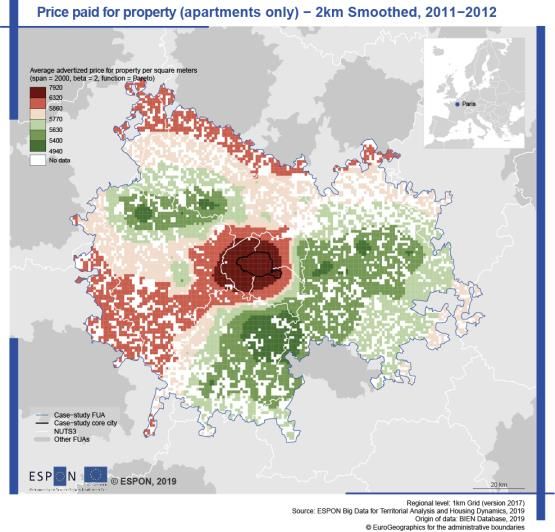
Final Report

This monitoring and tools activity is conducted within the framework of the ESPON 2020 Cooperation
Programme.

The ESPON EGTC is the Single Beneficiary of the ESPON 2020 Cooperation Programme. The Single
Operation within the programme is implemented by the ESPON EGTC and co-financed by the European
Regional Development Fund, the EU Member States and the Partner States, Iceland, Liechtenstein,
Norway and Switzerland.

This delivery does not necessarily reflect the opinion of the members of the ESPON 2020 Monitoring
Committee.

Authors
Renaud Le Goix, Université de Paris - UMS RIATE – CNRS Paris 75013 (France) – Project coordinator
Ronan Ysebaert, Université de Paris - UMS RIATE – CNRS (France) – Project manager
Timothée Giraud, CNRS, UMS RIATE – Université de Paris (France)
Marc Lieury, UMS RIATE – CNRS, University Paris 1 Panthéon-Sorbonne (France)
Guilhem Boulay, University of Avignon (France)
Thomas Louail, Géographie-cités (France)
José Ravier Ramasco, FISC-CSIC (Spain)
Mattia Mazzoli, FISC-CSIC (Spain)
Pere Colet, FISC-CSIC (Spain)
Thierry Teurillat, Haute-Ecole Arc (Switzerland)
Alain Segessemann, Haute-Ecole Arc (Switzerland)
Szymon Marcinczak, University Lodz (Poland)
Bartosz Bartosiewicz, Univeristy Lodz (Poland)
Elisabete Silva, Cambridge University (UK)
Sølve Baerug, Norwegian University of Life Sciences (Norway)
Terje Holsen, Norwegian University of Life Sciences (Norway)

Advisory Group
ESPON EGTC: Marjan Van Herwijnen (project expert), Caroline Clause (financial expert)

Information on ESPON and its projects can be found on www.espon.eu.

The web site provides the possibility to download and examine the most recent documents produced by
finalised and ongoing ESPON projects.

© ESPON, 2019

Printing, reproduction or quotation is authorised provided the source is acknowledged and a copy is
forwarded to the ESPON EGTC in Luxembourg.

Contact: info@espon.eu

ISBN: 978-99959-55-99-1
Final Report

 ESPON Big Data for Territorial
Analysis and Housing Dynamics

Wellbeing of European citizens regarding
      the affordability of housing.

Technical Guidance Document
          12/11/2019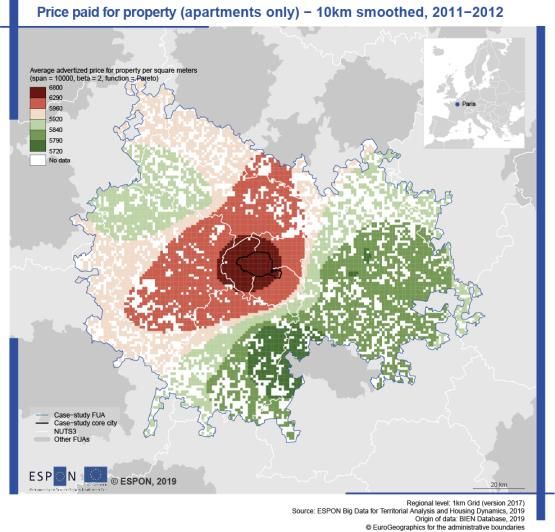
Table of contents
1      Introduction ........................................................................................................................ 1
2      Outlines of the conceptual and theoretical model ............................................................. 3
2.1 Theoretical model .............................................................................................................. 3
2.2 Harmonizing conventional and unconventional data to analyze the well-being ................ 3
3   Technical section: case-study analysis ............................................................................. 5
3.1 Transferability and reproducibility of the study: a narrative of a case-study analysis
    (Paris) ................................................................................................................................ 5
3.2 Conventional institutional data: Eurostat and National Statistical Institutes indicators ..... 8
3.3 Using unconventional institutional data to analyze the dynamics on property markets:
    data, methods, sample results ........................................................................................ 10
    3.3.1 Unconventional institutional data: data from Paris Chamber of the Notaries ......... 10
    3.3.2 Data aggregation in grid and LAU2 level ................................................................ 12
3.4 Using unconventional data sources: web-scraping of real-estate online listings ............ 15
3.5 Harmonised indicators (FUA and LAU2 scale) ............................................................... 18
    3.5.1 FUA indicators ......................................................................................................... 19
    3.5.2 LAU2 harmonized indicators ................................................................................... 22
    3.5.3 Mapping LAU2 harmonised indicators .................................................................... 23
3.6 Grid data and interpolation – spatial harmonisation issue to obtain a global and accurate
    picture of the real-estate market locally .......................................................................... 25
3.7 Comparing real-estate values to other big data sources (Airbnb)................................... 28
4   Summary of methodological and conceptual outputs. Next steps for further studies. .... 33

                                                                                                                                           i
ESPON Big Data for Territorial Analysis and Housing Dynamics / Guidance document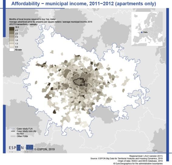
List of Maps
Map 3-1 Two resulting maps created with the R CODE 6 .......................................... 25
Map 3-2 Average advertised price at 1 km grid level – raw map ................................ 26
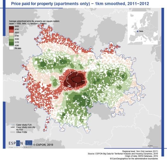
Map 3-3 Average advertised price at 1 km grid level – smoothed map (span = 2000m,
Pareto function, beta = 2) ............................................................................................. 28
List of Figures
Figure 3.1 - Overview of the workflow. ........................................................................ 6
Figure 3.2 - Data output : aggregation of relevant indicators at LAU2 and grid level
for 10 case-studies (extract). ........................................................................................ 15
Figure 3.3 - Get links to all ads of a given real estate Website.................................... 16
Figure 3.4 - Collect and sparse geospatial information ............................................... 17
Figure 3.5 – From basic indicators (transaction, web-scraped and institutional data) to
harmonised indicators at LAU2 scale .......................................................................... 23
Figure 3.6 – Comparing Airbnb and real-estate transactions (Paris). Density of Airbnb
offer (a.) compared to the density of transactions on apartment property markets (b.).
Residuals (c) of the linear regression (d). .................................................................... 29
Figure 3.7 – Comparing Airbnb and real-estate offer (Barcelona) .............................. 30
Figure 4.8 – Variogram of advertised price of real-estate property prices (euros/sq.
kilometer) in Barcelona according to distance............................................................. 36
Figure 4.9 – Average real-estate transaction prices (euros per square meters) in Paris
interpolated at several geographical scales (span parameter = 1000m, 2000m, 5000m
and 10000m) ................................................................................................................ 37
List of Tables
Table 3-1 – Listing of Eurostat available indicators relevant for characterising the
housing market ............................................................................................................... 9
Table 3-2 – Harmonised indicators created at FUA scale (real estate offer) displaying
synthetic indicators at FUA scale ................................................................................ 19
Abbreviations
ESPON European Territorial Observatory Network
ESPON EGTC ESPON European Grouping of Territorial Cooperation
EU European Union
LAU Local Administrative Unit
FUA Functional Urban Area
IDS Internet Data Sources
OECD Organisation for Economic Co-operation and Development
TOR Terms of reference
ii
ESPON Big Data for Territorial Analysis and Housing Dynamics / Guidance document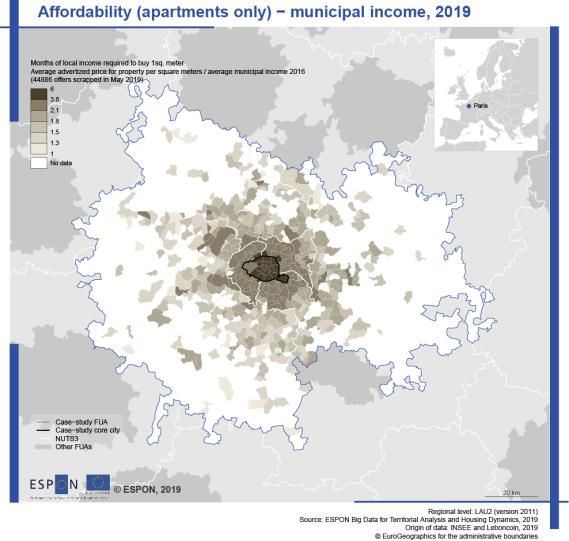
iii
ESPON Big Data for Territorial Analysis and Housing Dynamics / Guidance document
1 Introduction
This technical guidance document describes and demonstrates the methodological
framework applied to produce the ESPON EGTC Big Data for Territorial Analysis of Housing
Dynamics 2018-19 study, delivered as the Wellbeing of European citizens regarding the
affordability of housing report.

While in European larger cities, decent and affordable housing is increasingly hard to get
access to, the main goals of the study were:

    (1) to set up the framework towards the production of neighborhood and local spatial
        data;

    (2) to implement the framework with harmonized indicators, to examine the unequal
        spatial patterns of housing affordability in Europe;

    (3) to do it in a way that allows to compare between cities and within cities.

Its policy-oriented broader thinking is to analyze the spatial patterns of unequal local
affordability, as framed by the Action Plan of the Partnership on Housing of the EU Urban
Agenda that pushes for improved knowledge regarding affordability of housing.

The report addresses the housing elements of European policies through one major
issue: affordability, a concept defined as a gap between housing prices and households’
income (Friggit, 2017), and this gap has widened during the last decades. Since the 1990s,
housing prices have on average increased faster than the income of residents and buyers in
major post-industrial city-regions, but this is not ubiquitous. The scientific and policy goals of
the study aim at informing and locally mapping the increased affordability gap, a critical issue
for social cohesion and sustainability in metropolitan areas in Europe that impacts the well-
being of residents in European cities. To do so, the guidance document aims at
discussing the data collection and data models used for the production of the
delivered maps and data:

    •   The “Wellbeing of European citizens regarding the affordability of housing” datasets
        have been produced to analyse and map affordability in a selection of European
        cities.

    •   The report combines institutional data, and data harvested on real-estate
        advertisement websites. The issues with collecting and harmonizing such
        heterogeneous data sources (conventional and unconventional data) are discussed,
        as well as the methodology proposed to bridge such datasets.

    •   The datasets delivered are structured as spatial data with harmonized indicators that
        allow to compare between cities and within cities, to examine the unequal
        spatial patterns of housing affordability.

                                                                                                1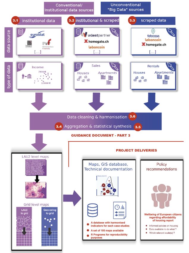
•    From the harmonized database, the study focuses on 9 case studies that cover a
         range of cities: from global and capital cities, down to medium-sized cities. Case
         studies offer a variegated sample, with several dynamics regarding housing market
         (gentrification process, tourism presence, housing crisis, etc.). Highlighting these
         various and complementary situations is relevant to carry out a first international and
         comparative study on housing dynamics in Europe based on local indicators. This
         guidance document will highlight the technical choices made to compare the
         indicators between cities in different countries.

The guidance document describes the data selection, harvesting and analysis process. It is
structured as follows:

    -    Section 2 overviews the conceptual and theoretical model used for standardisation
         and delivery of aggregated datasets, as well as data sources gathered, and described
         in the wellbeing report.

    -    Section 3 describes the data model and provides a description of the data collection
         and harmonisation processes. It discusses the technical choices and procedures for
         data harvesting, as well as the procedures for data harmonisation. This section gives
         insights on how results are technically produced and delivered, by the means of a
         workable example, elaborated with the Paris case study. This section of the
         guidance document is structured according to the workflow of the analysis, and
         narratively describes methods and R code used to implement the case study, in order
         to provide ESPON, stakeholders and policymakers with the conditions of
         reproducibility and transferability of the methodology used.1

    -    Section 4 summarizes methodological and conceptual outputs and elaborate on next
         steps for further studies.

    -    Several appendices complement the Technical Guidance Document, and are made
         available with the final delivery, for the sake of reproducibility and transferability: they
         include (1) an annex on harvesting data, with Python language libraries; (2) full
         code for the preparation of case-studies (R language), (3) a workable smaller
         example to demonstrate the diverse procedures used (RMarkdown html document)
         developed as a prototype demonstrator of the libraries and packages used for the
         project.2

1 Most programs used to prepare this report have been written in the R language, using a series of
packages that are documented in the Guidance document. R language is now a widely adopted open-
sourced standard programming language in spatial analysis, big data analysis, and statistics. Harvesting
websites also required the use of Python language (see Annex 1)
2 Full code in the R language is provided as used in data and spatial analysis (http://bit.ly/2XGEhiD).
Readers may also refer to an .html file, a RMarkdown document consisting in an archive of preliminary
stages of the project developments (D1_Draft_outline_guidance_document.html). This file was
constructed as a workable prototype example of the main packages used to produce analyse the
datasets and harvest data.

                                                                                                      2
2 Outlines of the conceptual and theoretical model
Starting with an explicit theoretical framework of affordability, the design of a harmonised data
structure is not an easy process and must follow specific methods and procedures. One issue
consists in defining an adapted methodology for combining conventional and unconventional
data sources. Another is to describe harmonisation procedures, which are not only technical,
but also conceptual. This section summarises some conceptual and theoretical elements that
are further elaborated in the Wellbeing Report, so as to introduce the technical choices of the
final data design.

2.1       Theoretical model
The theoretical model underlying the study starts with the problem of home values and market
values, and the widening gap compared to income (Aalbers, 2016; Friggit, 2017). The
theoretical framework from which we elaborate on stems an overarching conceptualisation of
affordability as part of a feedback loop between residential markets, value, assets,
wealth and vulnerability, thoroughly developed in Le Goix et al. (2019a); Le Goix et al.
(2019b). This theoretical framework is detailed in the Wellbeing report, section 1.2 and 1.3.
The report describes to effort towards collecting, documenting (metadata) local spatial
datasets to spatially analyse some critical issues:

      -    The increased affordability gap, a critical issue for social cohesion sustainability in
           metropolitan areas in Europe.

      -    The unequal access to housing markets.

      -    The increased inequalities stemming from declining affordability (i.e. higher price to
           income ratio)

2.2       Harmonizing conventional and unconventional data to analyze the
          well-being
One major issue is the lack of harmonised spatial data to map and monitor affordability
in Europe. There are plenty of institutional (tax, census), private (real-estate agents and
websites) and national or local data (parcels, local tax rolls). These are not harmonised and
interoperable. As demonstrated in the Wellbeing report (section 2.1), data by OECD and
Eurostat are disseminated respectively at the national and at the city levels, but the dataset
are far from complete in terms of thematic and geographical objects available to accurately
analyze housing dynamics. To bridge this data gap at the local level (LAU2 and FUA), we
collected and combined different spatial datasets and surveys which have so far been
employed separately. One issue consisted in defining an adapted methodology for
combining conventional and unconventional data sources.

                                                                                                3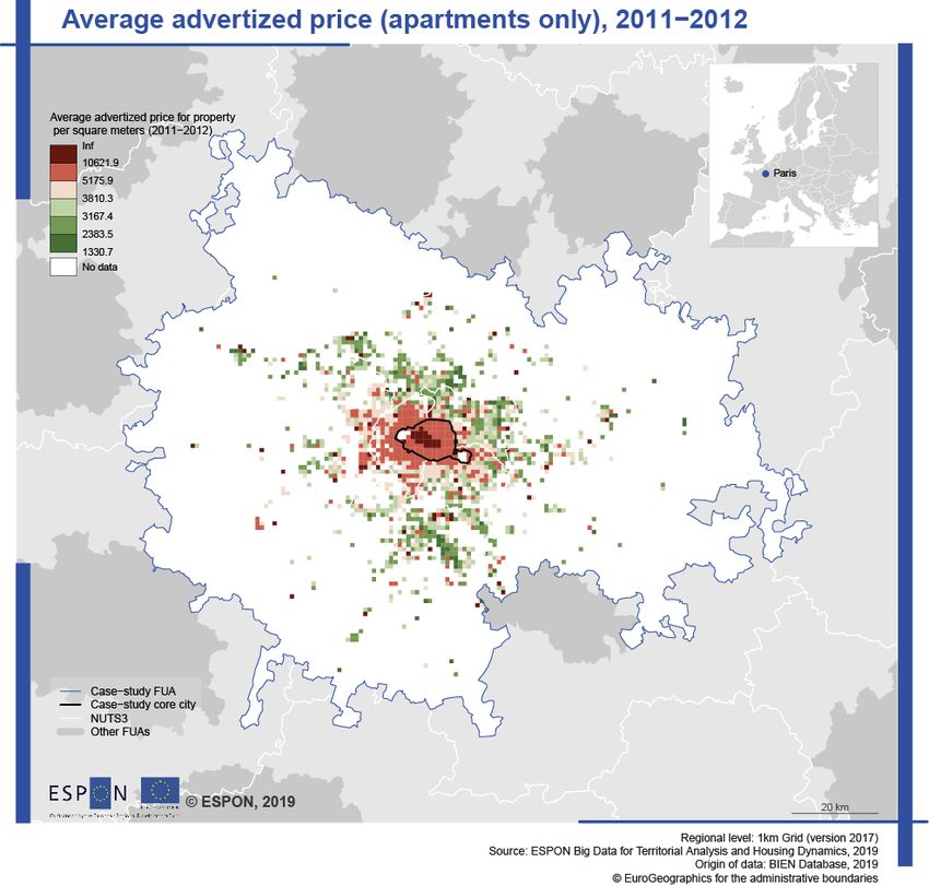
Definition of conventional and unconventional data

(quoted from the Wellbeing report, section 3).

Conventional data are provided by traditional statistical offices. This information, usually collected at
the individual scale and disseminated at several geographical aggregates, is subject to robust
processes of harmonisation and validation, by means of explicit conceptualisation of the future usage of
the data collected. Conventional data are usually realised through vintages (like censuses), but rely on
robust survey, samples and inferential statistics methodologies. Such data are disseminated with explicit
description of the fields and variable construction, definitions, sampling procedures, and statistical
robustness.

Unconventional data are extracted from various platforms and sources, and are often named “big
data”. Some might come from institutions, and are datasets collected for various administrative, fiscal
reasons, but that were not originally designed for socio-economic or demographic research. In many
ways, we incorporate them in research whereas such datasets have not been designed and/or
documented to do so (lack of metadata). Although originating from institutions, their robustness, as well
as inference on how such data describe the general population can often be questioned.

Many unconventional datasets are also derived from harvested data, made available by ISP (Internet
Service Providers) by the means of API, or scraped. Such unconventional data are often viewed as
interesting proxies to measure, and better understand spatial behaviors and territorial dynamics (Gallotti
et al.; Kitchin, 2013), and also as a means of providing higher spatio-temporal resolution data when
compared to institutional data sources (FP7 EUNOIA final report, 2015).

                                                                                                        4
3 Technical section: case-study analysis
For the purpose of the Wellbeing of European citizens regarding the affordability of housing
report we go beyond the aggregated territorial levels to understand intra-urban inequalities
between the cities. In term of data creation processing, three challenges have been
addressed in this research:
(1) Ensuring a data process which can be reproducible and transferable. It was mainly
done through and important documentation and programming codes.
(2) Delivering comparable and harmonised indicators for the selected cities and case
studies, 2 geographical levels are used to aggregate the collected data: the LAU2
level, and the 1km European reference grid.
(3) Covering the entire Functional Urban Areas, despite missing data and incomplete
datasets (mainly due to the absence of real-estate transactions or offers in the
periphery of FUA, which are mainly rural areas).
This section describes and demonstrates how we address each of these challenges, the
technical solutions implemented, and the data analysis design. All code for the study is made
available with the final delivery of the report. See “Programs” folder, containing R files,
delivered as a report appendix 3. The “Appendices” section of this document contains Python
code used for scraping purposes in France.
3.1 Transferability and reproducibility of the study: a narrative of a
case-study analysis (Paris)
We elaborate on the case-study of Paris as an ideal case study because of the availability of
institutional data4. We consider a variety of datasets:
- public conventional census data,
- unconventional institutional datasets, property-level data from the Paris Chamber of
Notaries (1996-2012, a sample of 1 million rows),
- unconventional harvested big data sources (real estate websites).
3 https://sharedocs.huma-num.fr/wl/?id=LPBWZm39VsZpXWnqIi9Q9HiTu0p5j9cF
4 The final guidance document describes the full methodology as a narrative summarizing the
data process and R code used from a complete case study. It differs from interim deliveries, that were
based on a prototype analysis designed as a RMarkdown document (Interim Delivery on Yvelines),
provided to describe and reproduce the overall workflow of analysis targeted. This interim document is
available online:
https://www.espon.eu/sites/default/files/attachments/Guidance_Document_201900426.pdf
5Harmonised and standardised variables are proposed, down to the local level (1 km grid).
Methods are applied to a set of geospatial data available. Section 3.3 documents the R
language code written for the purpose of the analysis: the goal is to demonstrate the
transferability and reproducibility of the methodology. The open-source R statistical
software uses open-source packages, that are well documented and maintained, and is
considered a standard environment in massive geospatial data analysis. By documenting the
R code with this narrative section, we document how the methodological framework has been
made transferable. It has been implemented with data from other case-studies to prepare
maps and visualisations for the Wellbeing report, availability of datasets permitting
(transaction data namely). In other words, all the indicators produced for each case-studies
stem from the same methodology, and are therefore made fully comparable within cities and
across cities.
Figure 3.1 - Overview of the workflow.
6In this section, we deliver a methodological narrative, in order:
- To describe the data collection process, both for conventional and unconventional
data sources.
- To describe and document the methodology employed to harvest datasets, using
APIs, and R packages s.a. `Cartography`, `SpatialPostion`, `rvest`, and `httr`, so as to
ensure reproducibility and transferability of the protocols.
- To describe a set of harmonised variables. Harmonised variables should be made
comparable between European cities, within cities and when data are available over
time. Ratios and standardized indices, such as affordability ratio are considered as
valuable alternatives to rough stock variables (s.a. price, surface), that are structurally
contingent to each country, city and local market contexts.
- To correct spatial and temporal data gap. Spatio-temporal information is sensitive to
two types of sampling issues: in space, and in time, therefore requiring the use of
interpolation procedures to ensure the quality and representativeness of the spatial
information produced. Spatial interpolation procedures are described, using for
instance the `Spatialposition` R Package.
To illustrate the project workflow, the narrative displayed in Chapter 3 aims at covering the
most important methodological aspects of harmonised data creation on real-estate market
(Figure 3.1) :
1. Data sources and data cleaning – A first issue highlighted is data collection from
the relevant information/data providers to target harmonized indicators. Conventional
census data are required to extract information at EU level on socio-economic
characteristics of case-studies and collect data on income, fundamental for estimating
real-estate affordability (Section 3.1). Institutional unconventional data are required to
describe residential property markets (Section 3.2). Data harvesting and web-
scraping (Section 3.3) has been critical in overcoming the situation where transaction
data simply does not exist. Where official transaction data exists, harvested data
allows to document the real-estate market offer (both property and rental market) vs.
actual transactions.
2. Harmonised indicators provision – Section 3.4 covers the design of harmonised
variables in a multiscalar perspective, produced at the local fine-grain geographical
city level (grid and LAU2) and the level of the entire FUA. Many are produced by
bridging institutional and census data.
3. Spatial harmonisation – Most of the indicators have been delivered at the LAU2
level. Section 3.5 explains the methodology and the interest to go beyond this
territorial level relevant for policy making by aggregating and interpolating the results
7in a 1km INSPIRE grid. This methodology offers a lot of advantages: by the means of
interpolation/smoothing techniques, we control for outliers and errors in the input
datasets. It also allows to better control for the MAUP effects (take into account the
number of real-estate offers/transactions in the calculation of price/square meters), it
estimates missing values using the assumption of spatial autocorrelation of real-
estate values. It finally allows to go beyond the LAU2 level which is basically too large
for observing existing inequalities for some cities defined by large territorial units,
such as Barcelona or Warsaw.
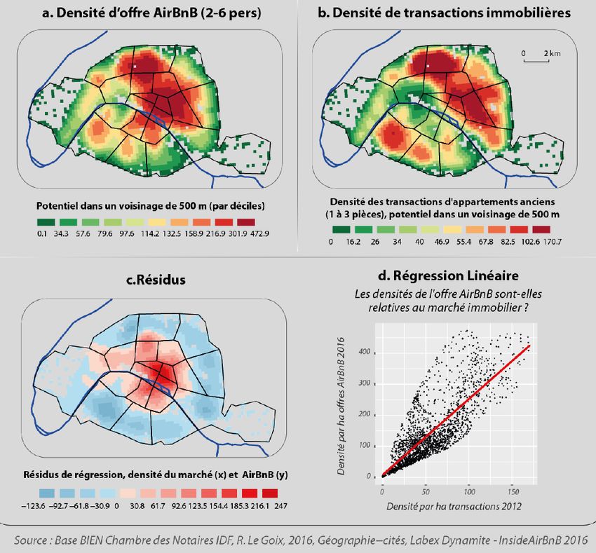
4. Data sources combination. Section 3.6 displays promising results for Paris and
Barcelona where some extra-combinations between unconventional data sources
have been tested for the sake of data exploration: real-estate offers (transaction
data in Paris, real-estate offer in Barcelona) and other big data source, like Airbnb.
Maps of statistical residuals produced clearly show the effect of Airbnb presence on
real-estate market (less offers than expected, all things being equal to the density of
real-estate offers or transactions) in touristic quarter (Center or Montmartre in Paris,
La Rambla in Barcelona).
This guidance document is concluded with highlights on how such data, maps and
interpretation realised have been aggregated together to produce harmonized indicators and
analysis at the three geographical levels of interest for this study, depending of data
availability: local grids, LAU2, central cities, FUAs.
3.2 Conventional institutional data: Eurostat and National Statistical
Institutes indicators
Two main categories of institutional data providers (“official statistics”) have been used:
harmonised European statistics (Eurostat) and national statistics (data coming from National
Statistical Institutes and Finance ministries).
EU statistics (Urban statistics, Eurostat) have been used to globally characterise selected
case-studies as regards to the other cities of Europe. Taking into account the availability of
data, 20 indicators at Core City and 14 at FUA level (less available information) have been
identified. These datasets include demographic indicators (age-structure), main households
characteristics, information related to the employment (economy tertiary oriented or not) and
other relevant factors to understand who lives in the cities. However, few information are
available on housing. It is only possible to extract one item of the EU perception survey: “is it
easy to find good housing in your city?”, which gives only a very rough qualitative assessment
of affordability by European citizens.
8Table 3-1 – Listing of Eurostat available indicators relevant for characterising the housing market
For measuring further comparable affordability indexes, the results of the EU-SILC survey
have also been used. This is the reference source for comparative statistics on income
distribution in the European Union. For this study, the first, the fifth (median) and the ninth
decile of income distribution have been gathered. This kind of information can be further (cf.
Section 3.4) used to analyse a time-normalised indicator of affordability (price to income
ratio), i.e. answering the following question: “How long the 10% poorest/median/10% richest
of the population have to work to buy/rent 1sq. kilometer in this city”? The choice of
thresholds has been made with regards to the needs for data standardisation to compare
national affordability between cities of several countries, which is not the case with income
statistics provided at local level by National Statistical Institutes.
In fact, LAU2 income data have also been gathered. It is especially useful for discussing on
affordability in a local context. A disclaimer shall however be disclosed regarding income
data. It is not recommended to compare local situation of affordability between cities of
several countries. Indeed, the methodologies for income computation varies from one country
to another. The ways income is imputed to persons or households differ between countries:
per capita or per households; before/after tax; with or without social benefits, etc. The
statistical parameters for aggregated income also differs in institutional data, some a median,
other are average income at LAU2 level. Nevertheless, local affordability indexes are still
highly relevant for comparing local affordability between cities of the same country (Avignon-
Paris / Madrid, Barcelona-Palma de Mallorca / or Lodz-Warsaw-Krakow separately), the
methodology of income calculation being generally harmonised at national level.
93.3 Using unconventional institutional data to analyze the dynamics on
property markets: data, methods, sample results
3.3.1 Unconventional institutional data: data from Paris Chamber of the Notaries
We use property-level data from the Paris Chamber of Notaries (1996-2012), provided to the
lead researcher by the Paris Notaries Services, a subsidiary of the Chamber of the Notaries,
under a research agreement with the Paris Chamber of the Notaries 5. This sample contains
transactions for the region and its suburbs, within the administrative limits of Ile-de-France
(roughly 1 million rows). All records contain information on the property amenities and pricing,
and series of understudied interesting variable on sellers and buyers, such as age, sex, socio-
economic status, national origin, place of residence, and some credit history related to the
transaction (95 indicators at transaction scale, cf R CODE 1).
###################### R CODE 1 #######################
#Import BIEN database (Chamber of Notaries) and analyse
dfdata str(dfdata)
'data.frame': 968695 obs. of 96 variables:
$ X.1 : int 1 2 3 4 5 6 7 8 9 10 ...
$ ID : int 1 2 3 4 5 6 7 8 9 10 ...
$ ACONST : int NA NA NA 1996 1996 1996 1996 1996 1996 1996 ...
$ ANNAIS_AC : int 1966 1967 1969 1961 1971 1945 1970 1937 1970 1973 ...
$ ANNAIS_VE : int NA NA NA NA NA NA NA NA NA NA ...
$ annee : int 1996 1996 1996 1996 1996 1996 1996 1996 1996 1996 ...
$ ANNEXE : chr "" "" "" "" ...
$ BATEAU : chr "" "" "" "" ...
$ BIARRON : chr "" "" "" "" ...
$ BICOMPADR : chr "ET 12" "ET 12" "ET 12" "zac des 2 golfs" ...
$ BICOMPNRVO : chr "" "" "" "" ...
$ BIDEPT : chr "77" "77" "77" "77" ...
$ BILIBVOIEO : chr "PAUL VALENTIN" "PAUL VALENTIN" "PAUL VALENTIN" "CHAMP DE LAGNY" ...
$ BINRQUARAD : chr "" "" "" "" ...
$ BINRVOIE : chr "10" "10" "10" NA ...
$ BINUCOM : chr "5" "5" "5" "18" ...
$ BITYPVOIE : chr "RUE" "RUE" "RUE" "LD" ...
$ CAVE : chr "1" "0" "1" NA ...
$ CODNAT_AC : chr "F" "F" "F" "F" ...
$ CODNAT_VE : chr "F" "F" "F" "F" ...
$ CSP_AC : chr "60" "60" "60" "51" ...
$ CSP_VE : chr "" "" "" "" ...
$ DATDEBBAIL : chr "" "" "" "" ...
$ DATMUTPREC : chr "26/01/1995 00:00" "26/01/1995 00:00" "26/01/1995 00:00" "02/11/1995 00:00" ...
$ DEPENDANCE : chr "" "" "" "" ...
$ DURBAIL : chr NA NA NA NA ...
$ ENCOMBRE : chr NA NA NA NA ...
$ ETAGE : chr "2" "2" "0" "2" ...
$ IMSURFTOTB : chr NA NA NA NA ...
$ INDIVI_AC : chr "N" "I" "N" "N" ...
$ INDIVI_VE : chr "N" "N" "N" "N" ...
$ insee : chr "77005" "77005" "77005" "77018" ...
$ IRIS : chr "770050000" "770050000" "770050000" NA ...
$ LARGFAC : chr NA NA NA NA ...
$ LOYANNU : chr NA NA NA NA ...
$ mois : int 6 5 7 3 3 3 3 3 3 3 ...
$ MTCRED : chr "59455" "63022" "51070" "74395" ...
$ NATNEGOC : chr "PR" "PR" "PR" "" ...
$ NBRBAT : chr NA NA NA NA ...
$ NBRCHSERV : chr "0" "0" "0" NA ...
$ NBRGARAGE : chr "0" "0" "0" "1" ...
$ NBRPIECE : chr "3" "3" "" "3" ...
$ NBRSALDB : int 1 NA NA 1 1 1 1 1 1 1 ...
$ NIVEAU : chr NA NA NA NA ...
$ Nom_commune: chr "Annet-sur-Marne" "Annet-sur-Marne" "Annet-sur-Marne" "Bailly-Romainvilliers" ...
$ NRPLAN1 : chr "426" "426" "426" "106" ...
$ NUMCOM_AC : chr "5" "294" "438" "81" ...
$ NUMCOM_VE : chr "372" "372" "372" "512" ...
$ PADEPT_AC : chr "77" "77" "77" "94" ...
$ PADEPT_VE : chr "77" "77" "77" "59" ...
$ PISCINE : chr "" "" "" "" ...
$ PRESCREDIT : chr "O" "O" "O" "O" ...
$ PXMUTPREC : chr "" "" "" "" ...
$ QUALITE_AC : chr "" "" "" "" ...
$ QUALITE_VE : chr "PR" "PR" "PR" "SC" ...
$ REFSECTION : chr "B" "B" "B" "AD" ...
$ REQ_AF_AC : chr "RP" "" "" "" ...
$ REQ_AF_VE : chr "" "" "" "" ...
$ REQ_ANC : chr "1" "1" "1" "2" ...
$ REQ_ASCENC : chr "" "" "" "N" ...
$ REQ_CHAUFC : chr "" "" "" "" ...
5 The transactions BIEN proprietary database was made available by Paris Notaire Service, on the behalf of
the Chamber of the Notaries, under an agreement contracted by the LabEx DynamiTe (ANR-11-LABX-0046) and the
Univ. Paris 1 Pantheon-Sorbonne.
10$ REQ_COS : chr "0" "0" "0" "0" ... $ REQ_DUREE : chr "17" "16" "18" "4" ... $ REQ_EPOQU : chr "B" "B" "B" "G" ... $ REQ_JARDIN : chr "" "" "N" "" ... $ REQ_MUT : chr "1" "1" "1" "1" ... $ REQ_NIVGAR : chr NA NA NA NA ... $ REQ_OCC : chr "1" "4" "3" "3" ... $ REQ_PM2 : num 945 NA NA 1593 1383 ... $ REQ_POS : chr "" "" "" "" ... $ REQ_PRIX : chr "47259" "50308" "51070" "89182.49" ... $ REQ_SURFT : chr "0" "0" "0" "0" ... $ REQ_VALUE : chr NA NA NA NA ... $ REQTYPBIEN : chr "AP" "AP" "AP" "AP" ... $ SDHOP : chr NA NA NA NA ... $ SEXE_AC : chr "M" "M" "M" "M" ... $ SEXE_VE : chr "" "" "" "" ... $ SHON : chr NA NA NA NA ... $ SITMAT_AC : chr "M" "C" "M" "M" ... $ SITMAT_VE : chr "" "" "" "" ... $ SURFHABDEC : chr "50" NA NA "56" ... $ TAUXTVA : chr "A" "A" "A" "H" ... $ TAXPF : chr "N" "N" "N" "O" ... $ TENNIS : chr "" "" "" "" ... $ TERRASSE : chr "N" "N" "N" "N" ... $ TXDRMUT1 : chr "3" "3" "3" "0" ... $ TYPAP : chr "AS" "AS" "DU" "AS" ... $ TYPBAIL : chr "" "AU" "" "" ... $ TYPGAR : chr NA NA NA NA ... $ TYPMAI : chr "" "" "" "" ... $ TYPMUTPREC : chr "A" "" "A" "A" ... $ TYPPRO : chr "P" "P" "P" "P" ... $ USAGE : chr "HA" "HA" "HA" "HA" ... $ VIABILISAT : chr NA NA NA NA ... $ X : chr "628337" "628337" "628337" "0" ... $ Y : chr "2436285" "2436285" "2436285" "0" ... ############################################################################################# The dataset is then filtered and a subset is prepared (ordinary transactions, residential only, apartments only, without null geographical coordinates, for 2011 and 2012), that represents 90000 observations. Nevertheless, some outliers may appear in the sample, due to data entry mistakes, which is a manual process for notaries in France). A first data cleaning consists in excluding to the sample exceptional values (1% lower and highest price/square meter transaction values). After data cleaning and filtering, the sample is reduced down to 76000 observations (cf. R CODE 2). ###################### R CODE 2 ####################### library(dplyr) # Convert required fields in numeric dfdata % # price > 1 eur filter(REQTYPBIEN=="AP" | REQTYPBIEN=="A" ) %>% #Appartements uniquement REQTYPBIEN=="AP" | REQTYPBIEN=="A" filter(X!=0) %>% filter(Y!=0) %>% # no 0 or 1 coordinates filter(X!=1) %>% filter(Y!=1) %>% # no 0 or 1 coordinates filter(annee == 2011 | annee == 2012) %>% filter(!is.na(X)) %>% filter(!is.na(Y)) # no NA coordinates # Prepare the data dfdata$REQ_PRIX
# Delete outliers
bornesQuantiles_prix  bornesQuantiles_prix
       0%        1%      2%        3%        4%        5%        6%        7%        8%        9%        10%
  200.000 1562.500 1800.000 1950.617 2062.500 2156.863 2245.895 2317.073 2385.285 2449.275          2500.000
      91%       92%     93%       94%       95%       96%       97%       98%       99%      100%
 9309.791 9528.302 9782.609 10000.000 10370.296 10789.474 11315.789 12071.193 13444.368 45000.000

dfdata = bornesQuantiles_prix[2] & PRIX_SURF
aggregated data are merged to EU reference layers thanks to their respective ID and exported to an Excel file. Transaction data are at this stage ready to be used for further analysis. ###################### R CODE 3 ####################### Library(xlsx) # Reference import (LAU2 and grids) FUA
col.names = TRUE, append = TRUE, row.names = FALSE, showNA = FALSE)

################### Aggregation LAU2 level
temp % count(insee))
colnames(temp)
Figure 3.2 - Data output : aggregation of relevant indicators at LAU2 and grid level for 10 case-studies
(extract).

3.4    Using unconventional data sources: web-scraping of real-estate
       online listings
Unconventional data are often viewed as interesting proxies to measure, and better
understand spatial behaviours and territorial dynamics, and also as a means of providing
higher spatiotemporal resolution data when compared to institutional data sources. Prior to
relying upon the unconventional data sources, it is important to assess their reliability, and to
assess how accurate the information provided is when compared to the long established
conventional data provision, an institutional statistically robust information collection data.

Gathering real-estate data on the internet (real-estate advertisement websites) requires to
follow a general procedure, which can be summarized as below:

A. Real-estate website identification – Real-estate websites are aggregators of
advertisement originating from real-estate agents, but also individuals, that generally have a
national coverage (the ads covers generally a single country). In other terms, it requires for
each country to define a listing of real-estate agencies in leadership situation (to obtain a
maximum of ads, well-structured and referenced). For France (Avignon, Geneva French part
and Paris), leboncoin.fr has been deemed of interest for this study, for its coverage and for its
data structure that allows a straightforward data harvesting effort, given the timeframe of the
study : in May 2019, it included 44886 real-estate offers (apartments only) and 20484 rental
offers in Paris.

B. Harvesting real estate online listings (ads) – Step 2 consists in getting the total number
of ads and determine the number of pages to scrape after having identified the relevant tags

                                                                                                       15
syntax in the URL query: as displayed in Figure 3.3 it corresponds to a geographical tag
(name of the NUTS3) and the type of offer tag (real estate offer / rental ; apartments and-or
houses, etc). Then, the method consists in exploring automatically all the adds included in all
pages of the query result. The output is a list of URLs to be harvested (one URL by offer).
Figure 3.3 - Get links to all ads of a given real estate Website
C. Identifying all the relevant information for listed properties. The next step consists in
preparing the script for each website to automatically fetch the data. It requires to harvest the
html webpage, and identify all the interesting attributes/tags to get (price, number of rooms,
surface, geographical location8…), as presented on Figure 3.4.
This is a tedious, very costly and time-consuming process that requires a lot of retro-
engineering. The cost and duration of the project allowed only for test drives and a few
months of collection, and some test platforms. We deliver a general methodology: it is
obvious that a script is valid for one real estate Website, considering the fact that they are
coded differently. Moreover, if the real estate Website change the organisation of the Web
page, the tags used in the script must be re-written. Such an iterative procedure is hand-
made, highly artisanal, and highly consuming in qualified worked-force, therefore
costly.
D. Data cleaning. The most common mistakes errors are duplicated ad’s (sometimes a real
estate ad can be published several times), absence of location coordinates or mistakes when
entering the real estate ad (area, price, etc.). Consequently, results obtained through the Web
scraping effort must be filtered. As an example for a case-study located in Yvelines in France,
8 Ideally, X/Y coordinates must be scrapped. For some real-estate website, like leboncoin.fr, it is
quite difficult to obtain this information. The LAU2 and the zip code are considered in this case.
16the 9934 observations collected resulted in 7460 unique and accurate records, with correct
location down to the municipality. The geocoding resulting from this procedure is in many
regards of poor quality compared to the locations provided by institutional data (transactions).
In the preliminary study, location data is provided by the website either as the city or
municipality (78%), and only a few ads are geocoded down to the address. In some other
cases location appear to be the location of the agency.
Figure 3.4 - Collect and sparse geospatial information
E. Data aggregation. Cleaned web-scraped data are then aggregated in targeted
geographical delineation (LAU2, grid), following the same methodology than the one used for
transaction data (Section 3.3. For some countries (Poland, Spain), it is possible to have
accurate X/Y location and it is consequently possible to aggregate real-estate offers at grid
level; for other countries, like in France with leboncoin.fr, X/Y location of real-estate offers is
not directly available, due to the design of the webpage. Harvested data can only be
aggregated at LAU2 scale for French real-estate offers.
173.5 Harmonised indicators (FUA and LAU2 scale)
Following the data collection/cleaning procedures (steps 3.3 and 3.4), a dataset is created (as
a ‘sf’ object in R), which includes all the information required to launch the analysis,
respectively:
- Official geometries (LAU2 and grid)
- Income data (municipal and national income data)
- Aggregated transaction data, if available (rooms, surface, price, debt contracted)
- Aggregated web-scraped data for property sales (rooms, surface, price)
- Aggregated web-scraped data for property rental (rooms, surface, price)
With this structured information, it is possible to launch the analysis on the housing market
and produce harmonised indicators combining conventional, institutional and unconventional
data sources as exemplified in R CODE 4. This section provides examples on how to match
data contained in transactions and other web-scraped data sources, and how to combine
them to external sources, like municipal income (coming from National censuses) or national
income (EU surveys)9.
The first series of harmonised indicators to be built informs on the main characteristics of the
housing market: size (surface, number of rooms) of the properties (transactions, offer, rental),
number of offers, price per sq. meters of local markets. This information gives important
insights to document the heterogeneity of real-estate market segments in case-studies.
The second series of indicators combine prices, to compare housing
prices between and within case studies. These are variables of interest to get an overarching
understanding unequal access to housing: advertised price, income, debt, for instance. To
better understand inequalities on housing markets, we start with nominal price, and then
produce harmonized variables, based on ratios, s.a. price-to-income, to analyze affordability;
and debt-to-value, a proxy for inequalities stemming from equity capital availability of
households (data available for French case-studies only). Using municipal income allows to
highlight the financial effort that local households have done to get another property or
property rental on local real-estate market. On the other hand, the use of national income
questions on the effort that a standard household should do to access the local real-estate
market studied in the case study, highlighting how inaccessible a metropolitan market can be.
The section describes and documents the harmonized indicators produced at the FUA level,
than at the LAU2 levels, and finally at the 1k Grid level.
9 The use of national income provided by EU surveys allows namely to overcome the
heterogeneity of national income definitions.
183.5.1 FUA indicators
One of the aims of the study consists also in producing statistical synthesis of transaction
data at FUA levels (all Paris FUA unit, with available data). This is done with the HousingStat
function, created for the project and described below (cf R CODE 4), which computes 29
indicators at FUA scale (using the LAU2 raw dataset, and aggregating these indicators using
weighted quantiles) relevant for discussing on housing characteristics and affordability:
• Transaction number (number)
• Surface of property (Q25, Q50, Q75, average)
• Number of rooms (Q25, Q50, Q75, average)
• Price paid (Q25, Q50, 75, average)
• Price paid per sq. meter (Q25, Q50, Q75, average)
• Time required to buy one square meter with municipal average income 10 (10% of the
poorest-richest population + median income)
• Time required to rent one square meter according to municipal or national income
(10% of the poorest-richest population + median income)
• Debt contracted / transaction value.
The interest of this function is also to use it for web-scraped datasets and other case-studies,
as displayed below in the synthetic table of the well-being report. It allows consequently to
produce/update quite easily, data being available, statistical synthesis at FUA scale.
Table 3-2 – Harmonised indicators created at FUA scale (real estate offer) displaying synthetic
indicators at FUA scale de
Geneva (FR) /
Barcelona (ES)
Mallorca (ES)
Geneva (CH)
Avignon (FR)
STATISTICS
Warsaw (PL)
Annecy (FR)
Krakow (PL)
Madrid (ES)
Paris (FR)
Lodz (PL)
Palma
Year of 2019 2019 2019 2019 2019 2019 2019 2019 2019 2019
reference
Number of 1096 10801 39293 1595 9382 79227 147094 22040 44886 5397
offers
Surface Q25 132.1 71 73.4 73.6 66.3 94.55 93.57 103.4 47.4 76.5
Q50 186 82 104.2 103.2 87.7 143.33 132.61 145.9 62 98.5
Q75 276.1 123.5 165.7 160.0 130.5 226.25 199.13 230.4 77.5 141.1
AV. 374.3 105.1 140.9 137.5 116.6 234.57 190.13 401.7 74.8 119.9
Rooms Q25 NA 3.2 2.5 2.55 2.5 NA 2.74 NA 2.3 3.57
Q50 NA 3.9 3.5 3.53 3.4 NA 3.33 NA 3 4.44
Q75 NA 4.8 4.5 4.54 4.4 NA 4.16 NA 3.8 5.61
AV. 7.6 4.1 NA NA NA 3.37 3.52 3.38 3 4.65
Price Q25 1 184 282.9 116.1 62.3 89.7 209.3 233.7 242.1 209.1 167.8
10 Using statistics provided by National Statistical Institute.
19(thousands Q50 1 863 373.6 168.5 872.7 117.5 334.4 334.4 360.5 274.9 233.0
euros) Q75 3 076 500.4 280.8 143.4 178.0 590.7 507.8 587.3 371.3 344.8
AV 4 460 400.2 234.6 118.65 158.4 516.7 441.8 554.8 307.9 283.8
Price per sq. Q25 NA 3584.5 NA NA NA 1897.6 2193.6 1940.5 4138 1925
meters Q50 NA 4133.6 NA NA NA 2550.5 2722.8 2552.3 4764 2404
Q75 NA 4682.9 NA NA NA 3299.7 3388.9 3364.3 5474 2820
AV 11915 4002.8 1665.3 863.2 1357.8 2202.9 2324 1381.1 4118 2366
Price to LOC11 67.8 15.7 22.0 15.69 19.1 15.05 14.01 19.6 12.8 14.7
income Q1012 217.1 35.7 77.1 39.0 52.1 93.17 79.67 100.04 25.2 24.1
Q50 112.7 19.6 39.5 19.96 26.6 36.38 31.11 39.1 13.9 13.3
Q90 61.4 10.6 20.7 10.48 14 17.67 15.11 19.0 7.6 7.2
Time required LOC 2.2 1.8 1.9 1.27 2.0 0.77 0.88 0.59 2.1 1.48
to buy 1sq. Q10 7.0 4.1 6.6 3.41 5.4 4.77 5.03 2.99 4 2.41
meter
Q50 3.6 2.2 3.4 1.74 2.7 1.86 1.96 1.17 2.2 1.33
(month)
Q90 2.0 1.2 1.8 0.92 1.4 0.90 0.95 0.57 1.2 0.72
###################### R CODE 4 #######################
Library(survey)
Library(sf)
Library (housing) (This package created within the project imports reference layers for all the case studies of the
ESPON Housing dynamics project (Paris, Avignon, Barcelona, Madrid, Palma de Majorque, Warsaw, Lodz, Krakow
and Geneva). The mapping functions implemented allow to create an ESPON map with all the required styles (colors,
labels, etc.)
# This function is used for analysing case-study data at FUA level
# HousingStat Function
HousingStatsvymean(STAT[,rq25], svydesign(ids = STAT[,id] ,data = STAT[,rq25], weights = STAT[,tsum]))[1]) rooms_q50
Indicator
to real estate offer. In other terms, a high index can be interpreted as locations where
         the development of rental offers may be specifically interesting for real-estate
         owners.

Figure 3.5 – From basic indicators (transaction, web-scraped and institutional data) to harmonised
indicators at LAU2 scale

######################                        R CODE 5                 #######################
# Ratios to be combined
LAU2$PRICE_ASKED_SQ
discontinuities maps. It also offers several features that improve the graphic presentation of maps, for instance, map palettes, layout elements (scale, north arrow, title...), labels or legends. These packages allow for a certain level of automation of iterative tacks. See R CODE 6. All the maps produced for the Wellbeing report have been created using the same methodology discretization methodology: “q6”, which is a method using quantile probabilities (0, 0.05, 0.275, 0.5, 0.725, 0.95, 1). From a cartographic perspective, the interest of the thresholds it introduced for cutting the statistical series is twice: first, it allows to introduce a double colour palette (warm colours below the case-study median and cold colours above the median); second the maps created for all the case-studies are comparable: for each case-study it is possible to observe on the map the 5 % of the units with higher/lower values. This choice of thresholds is another way to make the results comparable within and across case-studies. R CODE 6 is designed to produce 2 types of maps: price to income ratio (local income, price paid) and advertised price to income ratio (with web-scraped data). All the maps produced have been realized using this methodology. As a consequence, it is possible to produce quickly a large set of maps for each case-study for analysing housing market characteristics in 10 case-study cities. ###################### R CODE 6 ####################### Library(cartography) Library(sf) Library (housing) # Import reference geometries used for the map (with indicators) city
# And the same with web-scraped data - Time required to buy 1 sq. meters locally
pdf(file = "../fig/10_LAU2_BUY_SQ_METERS_LOC.pdf",width = sizes[1]/72, height = sizes[2]/72,
useDingbats=FALSE, pointsize=15.3568)
hm_bg(city)
choroLayer(LAU2, var = "BUY_SQ_METERS_LOC", method = "q6",
col = carto.pal(pal1 = "taupe.pal", n1 = 6),
colNA = "white", border = "white", lwd = 0.1, legend.pos = "n",
add = T)
hm_top(x = city, title = "Affordability (apartments only) - municipal income, 2019",
source = "INSEE and Leboncoin, 2019", object = "LAU2")
legendChoro(pos = c(st_bbox(city$stripes[3,])[3] + (st_bbox(city$mainframe)[3] - st_bbox(city$zoomBox)[3]),
(st_bbox(city$mainframe)[2] + st_bbox(city$mainframe)[4]) / 1.975),
title.txt = "Months of local income required to buy 1sq. meter\nAverage advertized price for property per
square meters / average municipal income 2016\n(44886 offers scrapped in May 2019)",
title.cex = 0.6, values.cex = 0.5, cex = 0.8,
breaks = getBreaks(LAU2$BUY_SQ_METERS_LOC, method = "q6"),
col = carto.pal(pal1 = "taupe.pal", n1 = 6),
nodata.col = "white", values.rnd =1)
dev.off()
#############################################################################################
Map 3-1 Two resulting maps created with the R CODE 6
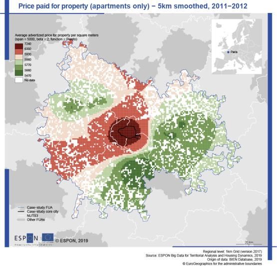
3.6 Grid data and interpolation – spatial harmonisation issue to obtain
a global and accurate picture of the real-estate market locally
For each case-study, at least one indicator has been aggregated at 1 km grid level. The
resulting raw map (Map 3-2) for Paris reveals three phenomena which may affect the
interpretation and the dissemination of the map:
- High spatial heterogeneity: despite data cleaning (exceptional values), spatial
structures are not clear: in the suburbs, high values are closed to lower ones. In
suburban areas especially, because of the fragmented structure of the built
environment and lower densities, classical econometric hypothesis regarding spatial
autocorrelation of property prices are often unverifiable (Le Goix et al., 2019b).
25- Missing values. It can be due to a lack of transaction in some grid cells or the
impossibility to display the data considering the fact that the number of observed
transaction is below the confidentiality threshold allowed by the Chamber of Notaries
database: it is not possible to disseminate data (datasets, or data displayed on maps)
below a given number of 5 transactions by territorial units (at LAU2 or grid level)
coming from the Chamber of Notaries database.
- Impossibility to disseminate the data as such, also due to confidentiality threshold.
Map 3-2 Average advertised price at 1 km grid level – raw map
Grid interpolation allows us to estimate a potential price in adjacent cells, with assumptions
regarding the spatial interactions between transactions. To offset these limitations, we use a
combination of a 1km grid and techniques of interpolation, following the assumptions of
Stewart’s potential, using the `SpatialPosition R package (Commenges et al., 2015). For
examples and detailed discussion of methodology regarding data processing, gridding,
interpolation, and mapping, see (Le Goix et al., 2019b).
The use of interpolation and estimation procedures allows to better control the quality and
representativeness of the spatial information produced, which is an estimation of the price, i.e.
a potential price. To do so, we used ‘SpatialPosition’, a R package allowing to compute
Stewart potential.
The Stewart potentials of population is a spatial interaction modeling approach which aims to
compute indicators based on stock values weighted by distance. These indicators have two
26main interests: first, they produce understandable maps by smoothing complex spatial
patterns; second they enrich the stock variables with contextual spatial information (Giraud,
Commenges, 2019). At the European scale, this functional semantic simplification may help
to show a smoothed context-aware picture of the localized socio-economic activities. It is also
a convenient methodological solution to offset the risk of Modifiable Area Unit Problem
(MAUP).
To interpolate and create Stewart potential, several steps are iterated, as displayed in the R
CODE 7:
• We create a distance matrix between the grid cells. Several methods for measuring
the distance can be considered: functional distances (time-road distance for
instance) or mathematical distance (Euclidian distance, Manhattan distance). Here
the Manhattan distance is considered, also called “taxi-distance”, especially useful
for city networks.
• We compute the potential according to a specific spatial interaction function. The
function inputs the matrix distance calculated above, known observations to
computes the estimates (sum of price paid and sum of property surface for
Paris), spatial interaction function (Pareto or Power law), span (distance where the
density of probability of the spatial interaction function equals 0.5 – 2000 m) and a
beta parameter (impedance factor for the spatial interaction function).
The parameters used for the analysis (2000m for the span, Pareto for the spatial
interaction function, 2 for the beta) are justified by the resolution of the grid (1km) and a
review of the literature on spatial characteristics of real-estate information, and semi-variance
tests performed on the datasets.
The Map 3-3 is the result of this harmonisation. It allows to go beyond the LAU2 delineation,
overcome the MAUP effect, and interpolate values ceteris paribus the number of observed
transactions and yields a global and accurate picture of the real-estate market on Paris FUA.
###################### R CODE 7 #######################
library(SpatialPosition)
library(sf)
## Create dist matrix (manhattan dist)
cGRIDYou can also read