Smartphone pressure data: quality control and impact on atmospheric analysis - Recent
←
→
Page content transcription
If your browser does not render page correctly, please read the page content below
Atmos. Meas. Tech., 14, 785–801, 2021
https://doi.org/10.5194/amt-14-785-2021
© Author(s) 2021. This work is distributed under
the Creative Commons Attribution 4.0 License.

Smartphone pressure data: quality control and impact on
atmospheric analysis
Rumeng Li1 , Qinghong Zhang1 , Juanzhen Sun2 , Yun Chen3 , Lili Ding4,5 , and Tian Wang4
1 Department  of Atmospheric and Oceanic Sciences, School of Physics, Peking University, Beijing 100871, China
2 National Center for Atmospheric Science, Boulder, Colorado, United States
3 National Meteorological Center, Chinese Meteorological Administration, Beijing 100080, China
4 Moji Co., Ltd, Beijing, 100015, China
5 Theme Tech Inc, Beijing, 100020, China

Correspondence: Qinghong Zhang (qzhang@pku.edu.cn)

Received: 14 May 2020 – Discussion started: 27 July 2020
Revised: 23 November 2020 – Accepted: 10 December 2020 – Published: 2 February 2021

Abstract. Smartphones are increasingly being equipped with       1   Introduction
atmospheric measurement sensors providing huge auxiliary
resources for global observations. Although China has the
highest number of cell phone users, there is little research     A lack of high-resolution observational data is one of the ob-
on whether these measurements provide useful information         stacles that limits the advance of numerical weather predic-
for atmospheric research. Here, for the first time, we present   tion (Bauer et al., 2015). This limitation can be extended to
the global spatial and temporal variation in smartphone pres-    all areas in atmospheric research. In recent years, many new
sure measurements collected in 2016 from the Moji Weather        observational technologies have emerged, including built-in
app. The data have an irregular spatiotemporal distribution      smartphone sensors, such as those for pressure, temperature,
with a high density in urban areas, a maximum in sum-            humidity and aerosols (Overeem et al., 2013; Snik et al.,
mer and two daily peaks corresponding to rush hours. With        2014; Muller et al., 2015; Droste et al., 2017; Meier et al.,
the dense dataset, we have developed a new bias-correction       2017; Zheng et al., 2018). With over 2.7 billion people in
method based on a machine-learning approach without re-          possession of smartphones (Bankmycell, 2019) and an in-
quiring users’ personal information, which is shown to re-       creasing trend in equipping smartphones with atmospheric
duce the bias of pressure observation substantially. The po-     measurement sensors, smartphone data can potentially be an
tential application of the high-density smartphone data in       auxiliary resource for global, high-density observations ca-
cities is illustrated by a case study of a hailstorm that oc-    pable of resolving convective-scale features with a resolution
curred in Beijing in which high-resolution gridded pressure      lower than 2 km (Mass and Madaus, 2014).
analysis is produced. It is shown that the dense smartphone         The smartphone sensors monitor atmospheric parameters
pressure analysis during the storm can provide detailed infor-   and convert them into electrical signals which can then be
mation about fine-scale convective structure and decrease er-    collected by different platforms, such as mobile weather
rors from an analysis based on surface meteorological-station    applications. Low-cost smartphone sensor data have been
measurements. This study demonstrates the potential value        used in several atmospheric research studies. Overeem et
of smartphone data and suggests some future research needs       al. (2013) and Droste et al. (2017) used smartphone battery
for their use in atmospheric science.                            data to study air temperature and their application to urban
                                                                 heat islands. Snik et al. (2014) mapped atmospheric aerosols
                                                                 using smartphone spectropolarimeters. Surface pressure is
                                                                 one of the most useful variables because it can reflect infor-
                                                                 mation about the whole atmospheric column and is less sen-
                                                                 sitive to the observational background (e.g., indoors/outdoors

Published by Copernicus Publications on behalf of the European Geosciences Union.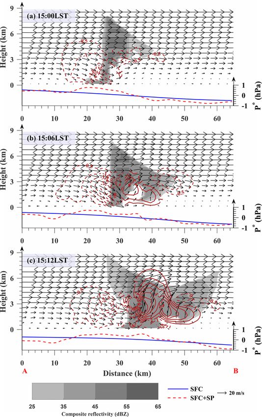
786                                                                                           R. Li et al.: Smartphone pressure data

Figure 1. The workflow for smartphone pressure data quality control and preprocessing. See text for details.

Table 1. Parameters used for machine learning.

   Data type/source             Field                                                                   Description
   Smartphone                   Gridded pressure at each smartphone site                                Pressure to be corrected
                                Longitude                                                               Location information
                                Latitude                                                                Location information
                                Time                                                                    Time information
                                Land cover                                                              Geographical information
                                Number of pressure observations aggregated at each smartphone site      Data uncertainty
                                Standard deviation of pressure observations at each smartphone site     Data uncertainty
                                Distance from domain center                                             Additional location information
   Automatic weather station    Pressure observation interpolated to each smartphone site               “True” pressure

or the influence of the underlying surface versus other vari-
ables like temperature and wind; Mass and Madaus, 2014;
Hanson, 2016); therefore, smartphone pressure data have re-
ceived considerable attention from researchers. In addition to
applications in weather forecasting (Mass and Madaus, 2014;
Madaus and Mass, 2017; McNicholas and Mass, 2018b;
Hintz et al., 2019), smartphone pressure data can be used to
monitor atmospheric tides (Price et al., 2018).
   While smartphone pressure data may have potential value,
they require validation and quality control before use. Price
et al. (2018) and Hintz et al. (2019) showed that, al-
though the variability between smartphone pressure data
and meteorological-station observations is highly correlated,
                                                                        Figure 2. Locations of global pressure observations in 2016 from
there exists noticeable bias. Price et al. (2018) calibrated the
                                                                        the Moji Weather application.
long-term stable bias using a one-point calibration method,
while Hintz et al. (2019) developed screening methods to re-
duce observational noise. Machine learning has also been ap-
plied to correct atmospheric pressure data (Kim et al., 2015,           consuming, especially for densely populated regions. It is
2016; McNicholas and Mass, 2018a). Most previous publi-                 therefore imperative to develop a new method that can ef-
cations on smartphone data calibration adopted a user-based             ficiently calibrate smartphone pressure bias while protecting
approach which required the identification of each unique               user privacy. It is worth noting that the need for such an effort
user and personal information. However, this raises privacy             has been recognized by other researchers, and similar efforts
and ethical issues that pose a concern to the public. As high-          are being undertaken (McNicholas, 2020).
lighted by Muller et al. (2015) and Mooney et al. (2017), col-             China has one of the world’s most densely distributed
lecting as little personal information as possible and keeping          smartphone user bases (Bankmycell, 2019) which can po-
raw data private are guiding principles of privacy preserva-            tentially produce highly dense observations. In this paper,
tion. Moreover, without a stable data collocation platform,             we present, for the first time, a year-long dense and exten-
performing user-based calibration can be time and resource              sive smartphone dataset collected by the Moji Weather app,

Atmos. Meas. Tech., 14, 785–801, 2021                                                       https://doi.org/10.5194/amt-14-785-2021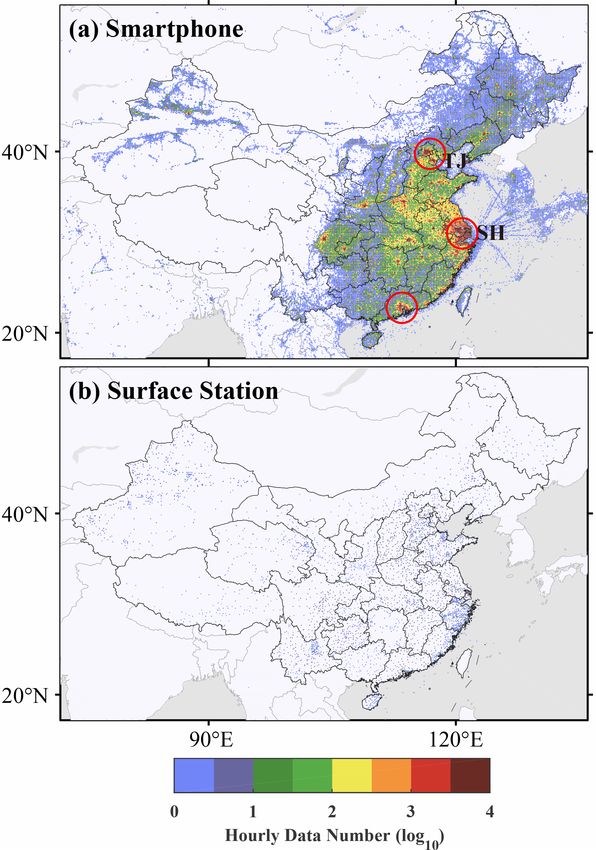
R. Li et al.: Smartphone pressure data                                                                                             787

Figure 3. Hourly pressure observation counts (log10 transformed)
averaged over the year 2016. Data are binned into a 0.1◦ × 0.1◦
grid.

which is developed and operated by the internet environmen-
tal meteorological corporation Moji. The Moji Weather app
is a popular smartphone weather app used in many countries
with a 53.90 % market share and more than 500 million users,
as well as over 100 million weather queries made every day
(Moji, 2019a, b). In the present study, we use the Moji smart-
phone pressure data for all of 2016 to show the spatial and
temporal distribution of the dataset. With this highly dense
network, we demonstrate the feasibility of a new machine-
learning bias-correction method that does not require users’       Figure 4. (a) Hourly pressure observation counts (log10 trans-
private information, thereby ameliorating ethical issues. The      formed) averaged over the year 2016. (b) Same as (a) but for the
dense network also makes it possible to study the detailed         Chinese Meteorological Administration (CMA) surface stations.
structure of atmospheric convection, which is demonstrated         Data are binned into a 0.1◦ × 0.1◦ grid in (a) and (b). The location
in this study by applying the bias-corrected data to the fine-     of the port of Shanghai and the port of Tianjin are labeled as “SH”
scale analysis of a hailstorm that occurred in Beijing.            and “TJ” in (a). The red circles indicate the urban agglomerations of
   This paper is organized as follows. Sect. 2 describes the       (from north to south) Beijing–Tianjin–Hebei region, Shanghai and
data and methods used in our research. The statistical char-       nearby cities, and Guangzhou and nearby cities.
acteristics of this dataset, bias-correction results and its ap-
plication to a hailstorm case are presented in Sects. 3, 4 and
                                                                   ventional stations) collecting meteorological data across the
5, respectively. Conclusions and discussion are given in the
                                                                   country, but only 13.32 % of the stations make pressure ob-
final section.
                                                                   servations. These weather station surface data are used as the
                                                                   authentication for the bias correction of smartphone pressure
2     Data and methods                                             data and for the verification of the surface analysis. (3) Land-
                                                                   use and land-cover data for China in 2015 at a resolution
2.1    Data description                                            of 1 km were accessed via the Data Center for Resources
                                                                   and Environmental Sciences, Chinese Academy of Sciences
Three types of datasets were used to perform this research.        (RESDC; Xu et al., 2018). These geographical data provide
(1) Pressure data were collected by a smartphone mobile            additional information necessary for our machine-learning-
weather application every second in 2016. The application          based bias-correction method.
collects longitude, latitude, time and pressure data for each
user without an unencrypted or encrypted ID. (2) Pressure
data were collected every 5 min by CMA (Chinese Mete-
orological Administration) in 2016. There are 68 909 sta-
tions (including automatic weather stations, AWSs, and con-

https://doi.org/10.5194/amt-14-785-2021                                                  Atmos. Meas. Tech., 14, 785–801, 2021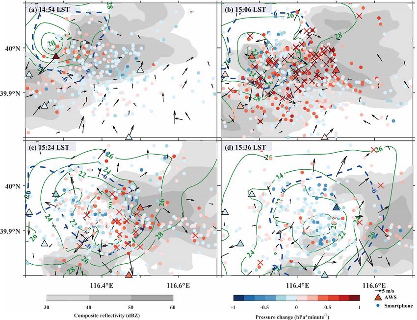
788                                                                                          R. Li et al.: Smartphone pressure data

Figure 5. (a) Seasonal variation in global hourly counts of smartphone data for each month. (b) Diurnal variation in global smartphone data
counts. (c) Annual mean hourly data count at different local standard times (LSTs) and months.

2.2   Quality control and preprocessing                                 dividual smartphone observation points are binned into spe-
                                                                        cific sites with fixed locations to eliminate the need for user
                                                                        IDs. The bias correction is then conducted on the aggregated
The quality-control and preprocessing procedure of the                  data in a 0.0001◦ × 0.0001◦ grid box (∼ 10 m × 10 m). In the
smartphone pressure data is described as follows. A work-               rest of this paper, the aggregated data points will be referred
flow diagram is shown in Fig. 1 summarizing the main pro-               to as “smartphone sites” for convenience. The next step in
cesses of the procedure. First, a gross check is conducted;             the quality-control procedure is a neighborhood check within
pressure values lower than 890 hPa or higher than 1080 hPa              each area of 0.01◦ × 0.01◦ latitude and longitude. Data with
are considered outliers and discarded (Kim et al., 2015;                values greater than 3 times the standard deviation of the mean
Madaus and Mass, 2017). The gross-checked data are re-                  pressure in the area are removed. Finally, we perform a sta-
ferred to as GC-data hereafter. Next, we perform tempo-                 tistical check. The boxplot approach is used to detect and
ral and spatial averaging. As described by McNicholas and               handle climatological outliers (Iglewicz and Hoaglin, 1993).
Mass (2018a) and Hintz et al. (2019), there is a spin-up time           For each boxplot, the upper quartile (Q3) is 75 % for the
for each measurement, and location retrieval for smartphones            smartphone air-pressure data, and the lower quartile (Q1) is
has an estimation error. To reduce such temporal and spatial            25 %. Data that are 1.5 times the interquartile range (Q3–Q1)
errors, the GC-data are averaged within a specified window              above Q3 and below Q1 are removed. The quality-controlled
of time and space. The time window size is 5 min to match               data after all the above steps are referred to as QC-data here-
the temporal interval of the weather station data or 6 min to           after.
match the radar update interval whenever necessary. The spa-
tial window size is 0.0001◦ latitude and longitude, i.e., the in-

Atmos. Meas. Tech., 14, 785–801, 2021                                                      https://doi.org/10.5194/amt-14-785-2021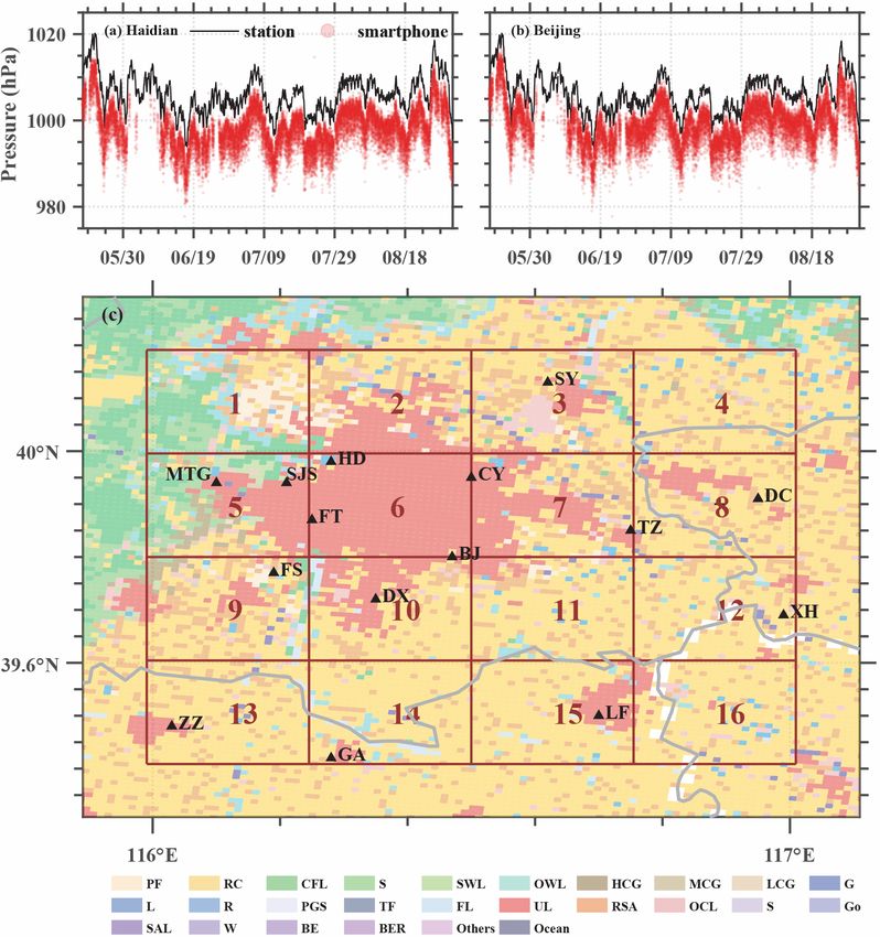
R. Li et al.: Smartphone pressure data                                                                                                  789

Figure 6. Spatial distribution of the standardized value of the data number at each site for each hour on 20 July 2016. The time is shown in
Beijing standard time (BJT). The standardized number is defined as the difference between the data number in this grid at a specific hour and
daily mean of the number divided by the standard deviation of the number. The dark gray color fill stands for the region in nighttime. Warm
colors indicate a rise in data volume, while cool colors indicate a decrease.

   It should be noted that the quality-control procedure above           correction method, that trains a single model in a specified
does not include elevation correction of the pressure data               area rather than for a single phone. Properly choosing the
not only because the Moji smartphone data do not include                 area size is crucial for the method to work effectively. It
the elevation information but also because the elevation-                should be small enough to ensure some degree of homo-
based pressure correction may contain notable errors due to              geneity in terms of geographical conditions, and on the other
the uncertainties in GPS elevation positioning (Kaplan and               hand, it cannot be too small because the machine learning
Hegarty, 2006; Ye et al., 2018) and in assumed pressure–                 requires a large enough data amount to work properly. Since
height relations. As an alternative, we use a neighborhood-              both users’ behavior and synoptic weather background dif-
based bias-correction approach, as described below, to cor-              fer among seasons, we conducted the training for each sea-
relate local pressure bias with the land-cover condition using           son. The data were randomly separated into training and test
the machine-learning technique.                                          sets (Overeem et al., 2013). The parameters used as input in
                                                                         the machine learning are listed in Table 1, including pressure
2.3   Bias correction                                                    from QC-data, longitude, latitude, time, land cover, number
                                                                         and standard deviation of raw data aggregated in a grid box,
Previous studies have demonstrated the importance of im-                 and distance of each smartphone site from the domain cen-
plementing appropriate validation and bias-correction proce-             ter. The land cover is used to provide geographic information,
dures before using smartphone pressure data in meteorologi-              which is an important input parameter for the neighborhood-
cal analysis (Muller et al., 2015; Hanson, 2016; McNicholas              based bias-correction approach. The number and standard
and Mass, 2018a). In our study, three machine-learning tech-             deviation of raw data aggregated in a grid box are used to
niques from the Waikato Environment for Knowledge Anal-                  provide data uncertainty. The true pressure value used for the
ysis (WEKA) suite (Witten et al., 2011) are used to cor-                 machine leaning is provided by the 5 min pressure observa-
rect the smartphone pressure data, and their effectiveness are           tions from AWS that are interpolated to each smartphone site.
compared. Unlike previous studies in which an individual                 To ensure some consistency in the two types of pressure data,
model was trained for each smartphone, in this study, we                 training data with a pressure bias (the difference of pressure
developed a method, named the neighborhood-based bias-

https://doi.org/10.5194/amt-14-785-2021                                                        Atmos. Meas. Tech., 14, 785–801, 2021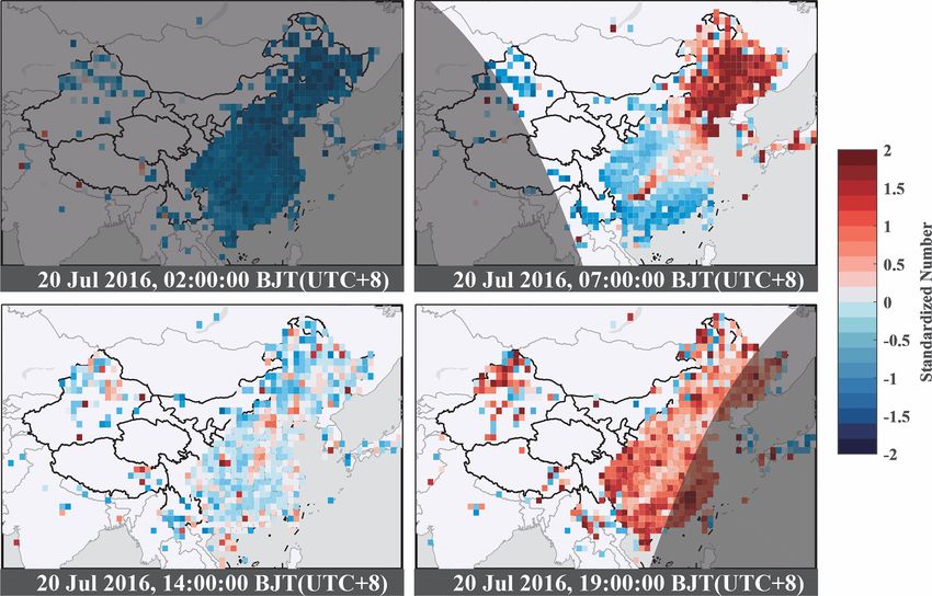
790 R. Li et al.: Smartphone pressure data
values between smartphone and AWS) greater than 15 hPa The analysis in subsequent refinement pass is described by
are removed. Eq. (3):
In order to evaluate the performance of the neighborhood-
based bias-correction method, three experiments with the g1 xg , yg = g0 xg , yg
following machine-learning methods, multilayer perceptron
P
wk (fk (xobs , yobs ) − g0 (xobs , yobs ))
(MP) (Pal and Mitra, 1992), support vector machine (SVM) + k P , (3)
k wk
(Shevade et al., 2000; Smola and Schölkopf, 2004), and ran-
dom forest (RF) (Breiman, 2001), were conducted, and their where g0 (xobs , yobs ) is the estimate value of g0 at an obser-
results will be compared later. vation point which is given by bilinear interpolation.
The objective analysis method described above was ap-
2.4 Objective analysis plied to generate analysis fields with a 1 km grid spacing
for a hailstorm case. In Sect. 5, we will show that the high-
It is well known that an accurate 2D surface analysis is ex- resolution analysis fields can be used to analyze fine-scale
tremely useful for nowcasting severe weather and studying pressure patterns for the hailstorm.
convective processes. Traditionally, this type of analysis is
mainly obtained from surface weather station observations.
However, since most of the weather stations do not have 3 Statistical characteristics
pressure measurements, the surface pressure analysis from
them can only depict gross features of large-scale flow. The 3.1 Spatial distribution
dense pressure observations from smartphones create an op-
portunity to improve the surface pressure analysis. In this We used the GC-data to analyze the spatial and temporal dis-
study, we use an objective analysis method modified from tribution of the smartphone data counts in 2016. The data
Barnes (1964) to conduct the analysis. The modified Barnes location map in Fig. 2 shows that smartphone data are dis-
analysis method, described below, interpolates randomly dis- tributed over nearly all continents, although most of the data
tributed data into a uniformly spaced coordinate system using counts occur in China with much higher data density (Fig. 3).
a two-pass successive correction method. The global mean density of the data is 40 per bin per hour,
If a variable fk is observed at a location (xobs , yobs ), then whereas in China, the density is 176 per bin per hour. The
the first pass analysis at a grid point g0 (xg , yg ) is obtained by hourly pressure observation counts for the entire year of 2016
Eq. (1): for China and its surroundings (black box in Fig. 2) are
binned using a 0.1◦ × 0.1◦ grid and shown in Fig. 4a, which
P
wk fk (xobs , yobs ) indicates that the data density is higher in megacities, such as
g0 x g , y g = k
P , (1) the densely populated urban agglomerations of the Yangtze
wk
k River Delta (Shanghai and nearby cities), Pearl River Delta
(Guangzhou and nearby cities), and Beijing–Tianjin–Hebei
where the weight wk for the observation point is given by region (marked by red circles in Fig. 4a). Because people
Eq. (2): carry mobile phones while traveling internationally, ship tra-
r2
jectories can be seen from two ports, the port of Shanghai
exp − γ Lk 2 , r ≤ re
wk = , (2) (SH) and the port of Tianjin (TJ) (Fig. 4a), but the amount of
0, r > re data at sea is much lower than on land. However, in compari-
son with the surface observations of the Chinese Meteorolog-
where rk is the distance from the grid point (xg , yg ) to the kth ical Administration (CMA) (Fig. 4b), the amount and spatial
observation point; γ is the convergence factor which controls coverage of the smartphone data are remarkable in nearly all
the refinement between the two passes (Barnes, 1974) and regions.
lies between 0 and 1 (0 < γ ≤ 1); L is the length scale that
controls the rate of falloff of the weighting function; and re is 3.2 Temporal distribution
the radius of influence within which the observations have an
The seasonal and diurnal distributions of the GC-data are dis-
impact on the grid point. Different from the standard Barnes
played in Fig. 5 The data volume peaks during the North-
interpolation technique using a uniform length scale over the
ern Hemisphere summer and reaches a minimum in winter
analysis domain, an adaptive Barnes scheme is applied in this
(Fig. 5a, c). The annual mean data volume is 279 377 per
paper in which the length scale automatically adapts to data
hour, which far exceeds the value of 47 000 per day in Ko-
density, i.e., a spatially variable length scale is computed ac-
rean shown in Kim et al. (2015), suggesting a large user base
cording to the data density.
of the Moji Weather app. The data seasonality indicates that
people check the weather more frequently in summer than in
winter, owing to the fact that the app can only get the pres-
sure information when the network is available and when the
Atmos. Meas. Tech., 14, 785–801, 2021 https://doi.org/10.5194/amt-14-785-2021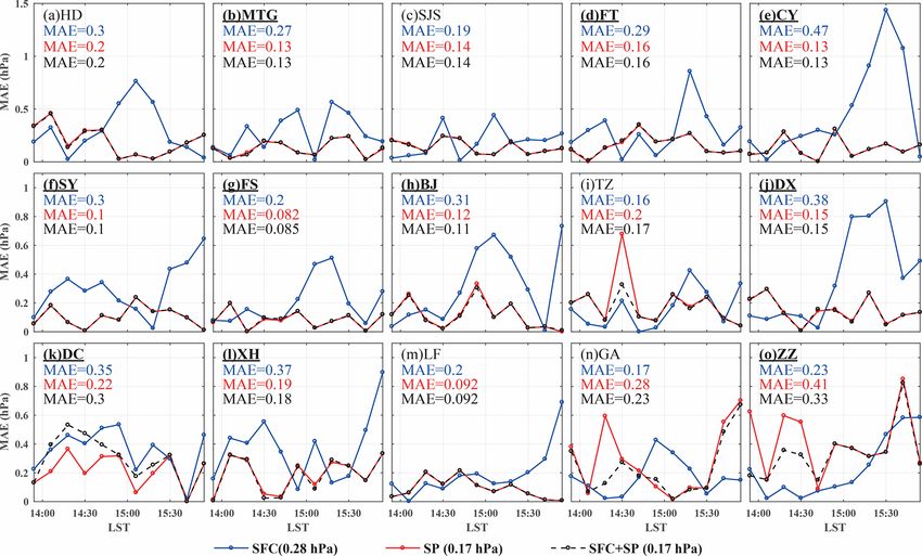
R. Li et al.: Smartphone pressure data                                                                                              791

Figure 7. Diurnal variation in the data volume for smartphone data on the day of the hailstorm (red line) and the annual mean value (blue
line) for 39–41◦ N, 115–118◦ E. Panels (a)–(d) show a 3D view of data counts in a 0.05◦ × 0.05◦ grid over 6 min (colored columns) before
each radar volume and radar echo (gray columns). The color and height of each column represent the value of the data count. BJ, Beijing;
TJ, Tianjin.

users open the app either on the front end or back end. The            nual mean hourly data within 39–41◦ N, 115–118◦ E are plot-
diurnal variation in global data volume (Fig. 5b, c) shows             ted in Fig. 7. The diurnal cycle on the day of the hailstorm
two peaks at 07:00 and 18:00 local standard time (LST), cor-           shows that, in addition to the two peaks in the morning and
responding to the rush hour in the morning and evening, re-            evening, another peak appeared at 16:00 LST with a data vol-
spectively. Additionally, there is a steep decrease in data vol-       ume 3 times that of the annual mean. A 3D view of the data
ume at night, which is consistent with a previous report that          volume and radar echo accumulated within 6 min (Fig. 7b–d)
smartphone data are inhomogeneously distributed through-               clearly shows a rise in data volume (Fig. 7b, d) as the storm
out the day (Hintz et al., 2019). The diurnal distribution char-       approaches Beijing and Tianjin and a drop after the storm
acteristic indicates that users tend to check the weather be-          passes (Fig. 7c), which demonstrates the influence of severe
fore going to work in the morning and getting off work in the          weather on human behavior.
evening. To demonstrate this more clearly, the spatial distri-
bution of the standardized value of the hourly data number at
each site is computed for 2 d and displayed in Fig. 6. Interest-       4   Evaluation of the bias-correction method
ingly, the data volume peak occurs earlier in northeast China,
which corresponds well with an earlier sunrise (Fig. 6b).              Three neighborhood-based bias-correction experiments,
   Analysis during a hailstorm that occurred in Beijing fur-           each using one of the aforementioned machine-learning
ther reveals that people respond promptly to severe weather            methods, were conducted on a domain covering Beijing and
events. The hailstorm occurred on 10 June 2016 as a squall             its surrounding area from May to August 2016. The machine-
line passed through Beijing city from 14:00 to 17:00 LST.              learning bias correction was performed in each of the subdo-
The hourly data volume on the day of the hailstorm and an-             mains in Fig. 8c using surface observations as the truth and

https://doi.org/10.5194/amt-14-785-2021                                                     Atmos. Meas. Tech., 14, 785–801, 2021
792                                                                                           R. Li et al.: Smartphone pressure data

Figure 8. (a, b) Pressure time series during the training period for the AWS (black line) and smartphones (red dots); smartphone pressure
was interpolated into station location using the inverse distance weighting method. (c) The domains of the machine-learning area. Shaded
areas are regional land use (PF, paddy field; RC, rainfed cropland; CFL, closed forest land; S, shrubbery; SWL, sparse woodland; OWL, open
woodlot; HCG, high-coverage grassland; MCG, moderate coverage grassland; LCG, low-coverage grassland; G, graff; L, lake; R, reservoir
pond; PGS, permanent glacier snow; TF, tidal flat; FL, flood land; UL, urban land; RSA, rural settlement area; OCL, other construction land;
S, sand; Go, Gobi; SAL, saline-alkali land; W, wetland; BE, barren earth; BER, bare exposed rock). Automatic weather stations (AWSs) with
pressure observations are shown by black triangles (HD: Haidian; MTG: Mentougou; SJS: Shijingshan; FT: Fengtai; CY: Chaoyang; SY:
Shunyi; FS: Fangshan; BJ: Beijing; TZ: Tongzhou; DX: Daxing; DC: Dachang; XH: Xianghe; LF: Langfang; GA: Guan; ZZ: Zhuozhou).

the smartphone input parameters listed in Table 1. The region           is consistent with the results of Price et al. (2018) and Hintz
was affected by the 10 June 2016 hailstorm and had a high               et al. (2019).
density of smartphone pressure observations (Fig. 7a–d).                   Figure 9 shows the mean absolute error (MAE) and com-
   Constrained by the requirements of adequate data samples             putation time at different training regions for the three meth-
and reasonable computation cost, we chose 16 subdomains                 ods; it is evident that the RF method is more accurate and
of 0.25◦ (longitude) × 0.20◦ (latitude) in size. The pres-              time saving. The computation times for subdomain 2 and
sure time series from two representative stations in Fig. 8a            subdomain 6 using the SMO method are more than 9 h. From
and b show that, although the trend in the weather station              this comparison, we have found that the RF algorithm is more
and smartphone is consistent, bias is clearly present, which            suitable for the neighborhood-based bias correction of smart-
                                                                        phone observations without requiring users’ personal infor-

Atmos. Meas. Tech., 14, 785–801, 2021                                                       https://doi.org/10.5194/amt-14-785-2021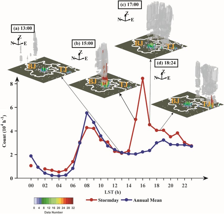
R. Li et al.: Smartphone pressure data 793
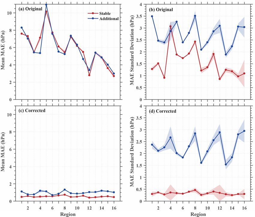
set and test set as stable sites and those only appearing in the
test set as additional sites. To quantify the performance of
bias correction, the domain-average MAE and standard devi-
ation of ensemble mean for the 16 subdomains are displayed
in Fig. 10 for the raw and bias-corrected data from both the
stable sites and the additional sites. The MAE was calculated
using data from the smartphone sites for each subdomain.
Comparing the MAEs between the raw (Fig. 10a) and bias-
corrected data (Fig. 10c), it is evident that the neighborhood-
based bias-correction method is capable of substantially re-
ducing the MAE not only for the stable sites but also for
the additional sites with slightly more reduction for the sta-
ble sites (from 5.95 to 0.53 hPa) than for the additional sites
(from 5.90 to 0.99 hPa). It is also shown that the method re-
duces the MAE spread by 78 % for the stable sites and by
16 % for the additional sites (Fig. 10b, d). A lower MAE
and spread reduction for the additional sites is not surpris-
ing because they are newly added data with shorter data
history and hence have fewer data samples (Fig. 11a, b).
Encouragingly, our results suggest that the neighborhood-
based method can partially mitigate the difficulty related to
recently added data with shorter data history. In compari-
son with the bias-correction method based on a single site,
the neighborhood-based method resulted in a substantially
smaller MAE (see Fig. 11c, d).
5 Impact of smartphone data on hailstorm analysis
High-density pressure observations can potentially help iden-
tify small-scale surface pressure patterns beneath a thunder-
storm (Johnson and Hamilton, 1988). Although the quality-
controlled gridded smartphone pressure data reduce the num-
Figure 9. (a) Mean absolute error (MAE) distribution at different ber of data points, they are still adequate to represent the fine-
training subdomains for different machine-learning methods (MP scale pressure patterns. In this section, we first show what
refers to multilayer perception method; SMO refers to support vec-
small-scale information the quality-controlled high-density
tor machine method; RF refers to random forest method). Panel
(b) is the same as (a) but for computation time.
pressure data at the smartphone sites (with a spatial resolu-
tion of 0.0001◦ or approximately 10 m) can provide and then
demonstrate the impact of the smartphone data on the grid-
ded 1 km pressure analysis that is obtained using the objec-
mation. Furthermore, we discovered that the random data tive analysis method described in Sect. 2.4.
separation into training set and test set can cause random er- Figure 12 shows a composite plot of radar reflectivity,
rors in the bias-corrected data; hence, in order to eliminate pressure changes calculated from surface weather station ob-
these errors, the correction procedure was repeated for 50 servations and from smartphone data, and wind and equiv-
times to generate an ensemble result. alent potential temperature from the station observations.
Collecting smartphone data through a weather app is con- To be consistent with the time interval of the radar volume
venient and common; however, the approach relies on the scan, the smartphone QC-data averaged every 6 min were
loyalty of users. Calibrating smartphone pressure individ- used to generate the 6 min pressure tendency. Further, be-
ually can be only applied to data from long-term users, cause the weather station data are at a 5 min interval, the
but it cannot be used for recently added users. In con- pressure change and temperature from these data are shown
trast, performing data correction for the aggregated data in at times closest to those of the radar volume scan. Since
a 0.0001◦ × 0.0001◦ grid box in a subdomain makes it possi- there are only 15 weather stations providing pressure obser-
ble to collect data from both user groups. In order to evaluate vations in this region, they are unable to locate the leading
the applicability of our method on data from both types of edge of the cold pool. In contrast, the smartphone pressure
users, we define the data sites appearing in both the training observations are much denser and hence are able to cap-
https://doi.org/10.5194/amt-14-785-2021 Atmos. Meas. Tech., 14, 785–801, 2021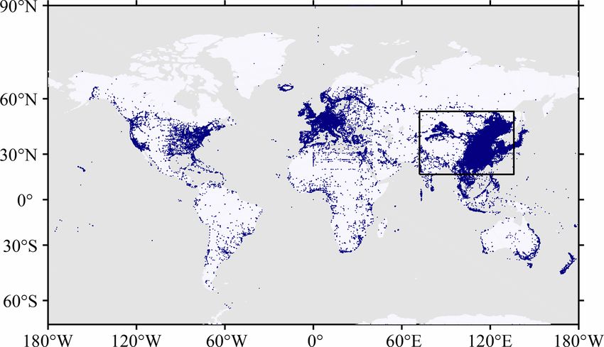
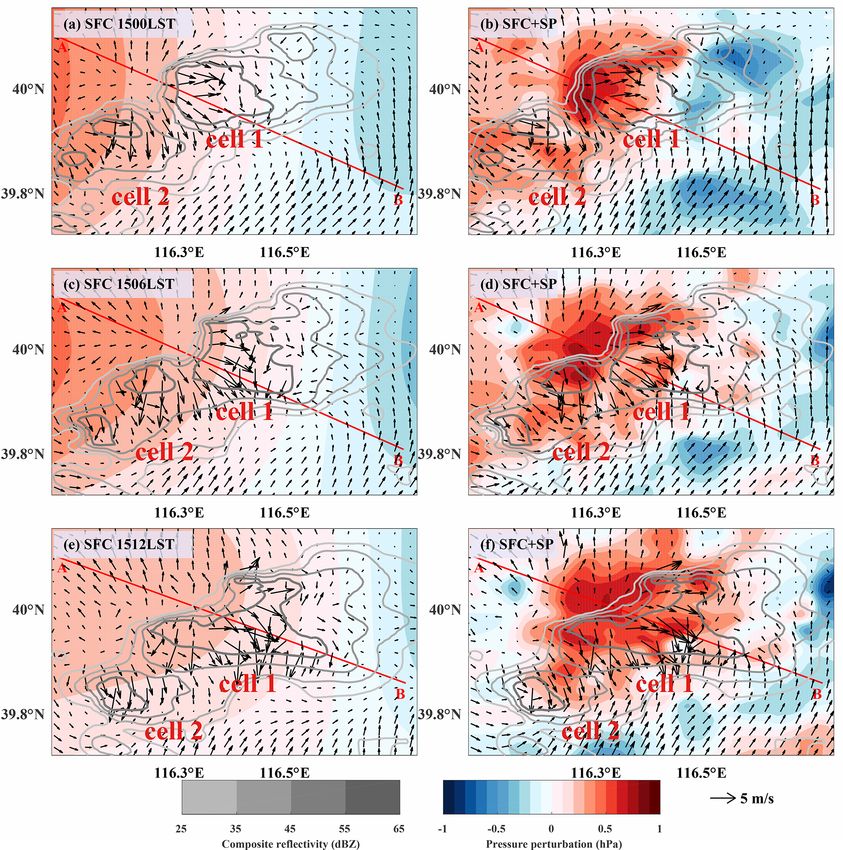
794                                                                                                 R. Li et al.: Smartphone pressure data

Figure 10. Distribution of domain-average mean absolute error (MAE; a, c) of ensemble mean and standard deviation (b, d) for different
subdomains for the original dataset (a, b) and the bias-corrected dataset (c, d). The line marked by dots is the ensemble mean value, and
shading is the double standard deviation ensemble spread. The red line is the result for stable sites, and the blue line is the result for additional
sites. See text for the definitions of stable sites and additional sites.

ture the fine-scale pressure change associated with the cold                 using both the station and smartphone data. The analysis grid
pool, as depicted in Fig. 12 by the “×” symbol represent-                    spacing is 1 km. Figure 13 shows the domain for surface anal-
ing the 6 min change in perturbation pressure (i.e., domain                  ysis and the locations of the Beijing radar and surface sta-
mean subtracted) greater than 0.52 mb. Compared with the                     tions.
cold pool leading edge identified by θe , following Schlem-                     The analyses of perturbation pressure (i.e., relative to do-
mer and Hohenegger (2014), from the analysis of surface                      main mean) from the experiments SFC (Fig. 14a, c, e) and
observations, the leading edge of the cold pool based on                     SFC + SP (Fig. 14b, d, f) are compared at 15:00, 15:06 and
the smartphone pressure change is about 10 km ahead at                       15:12 LST in Fig. 14. To illustrate the coupling between
15:06 LST (Fig. 12b) and quite close at 15:24 LST (Fig. 12c).                pressure and wind in the storm region, the wind field at
At 14:54 LST (Fig. 12a), the pressure change is largely neg-                 150 m from VDRAS (Variational Doppler Radar Analysis
ative ahead of the cold pool, whereas Fig. 12d mainly shows                  System) and the composite reflectivity observation are over-
negative pressure changes after the leading edge has passed                  laid. VDRAS is a rapid update analysis system based on
the area; both are consistent with the surface station observa-              the variational technique that blends radar radial velocity
tions but are more detailed.                                                 and surface wind observations to produce 3D wind analy-
   We conducted three objective analysis experiments using                   ses (Sun and Crook, 1997, 1998). We first note that the per-
the method described in Sect. 2.4 to demonstrate the poten-                  turbation pressure analysis from SFC + SP (right column)
tial benefit of using smartphone observations along with sur-                displays small-scale features in and around the storm that
face weather station observations to improve surface pressure                are absent in SFC (left column). The high center of pres-
analyses, i.e., the station observation experiment (SFC) us-                 sure perturbation is nearly collocated with the center of the
ing only weather station pressure observations, smartphone                   outflow near the northwest flank of the main body of the
experiment (SP) using only smartphone data, and SFC + SP                     storm system (Fig. 14b, d, f). The vertical cross sections

Atmos. Meas. Tech., 14, 785–801, 2021                                                             https://doi.org/10.5194/amt-14-785-2021
R. Li et al.: Smartphone pressure data                                                                                                    795

Figure 11. (a, b) Scatter plot of mean absolute error (MAE) versus the data number of observation sites for (a) stable sites and (b) additional
sites. (c, d) Scatter plot of station pressure versus bias-corrected pressure for (c) the neighborhood-based method and (b) single-site method
of one ensemble member. Averaged mean absolute errors (MAEs) of the two methods are shown in the plot.

shown in Fig. 15 through the line A–B (see Fig. 14) indicate              higher resolution of the smartphone data applied in this study,
that the high-pressure perturbation corresponds to the rear-              but further studies are needed to draw a definite conclusion.
flank downdraft aloft behind the intense radar echoes of the              Furthermore, the pressure analysis from SFC + SP provides
southeastward moving convective system. Although the rela-                more detailed information about storm evolution than what
tively low-pressure regions are seen in front of the convective           is shown in SFC. As the storm moves southeastward, the
system in both experiments, only the SFC + SP experiment                  cell in the southwest, denoted as cell 2 in Fig. 14, separates
captures the relatively low-pressure region northwest of the              into two (Fig. 14b), and the northern one merges into cell 1
system. The overall distribution pattern of pressure perturba-            (Fig. 14d, f). During the merging process, the high-pressure
tion in SFC + SP is consistent with the conceptual model of               region behind cell 1 becomes stronger and wider, which may
Markowski and Richardson (2010), but the current analysis                 indicate the enhancement of cell 1 in correspondence with
reveals that the surface high-pressure region and low-level di-           the increased downdraft and updraft, as shown in Fig. 15c.
vergence center slightly lag behind the center of the intense                Analysis accuracy for the two experiments was verified
reflectivity echoes rather than right beneath it, as in their con-        against the 15 weather station pressure measurements in the
ceptual model. We believe the difference results from the                 domain. In order to avoid dependence between the analysis

https://doi.org/10.5194/amt-14-785-2021                                                         Atmos. Meas. Tech., 14, 785–801, 2021
796                                                                                             R. Li et al.: Smartphone pressure data

Figure 12. The 5 min pressure change from surface stations (triangles) and the 6 min pressure change from smartphones (points), temperature
observations from surface station (green contour), wind field (black arrow), and composite radar reflectivity (shaded) during a hailstorm that
occurred on 10 June 2016 in Beijing, China. The station pressure change is shown at the time closest to that of the radar volume. The “×”
symbol marks the locations where the 6 min pressure change perturbation is greater than 0.52 hPa. The dashed blue line is the 1θe = −6 K
isoline from the analysis of surface observations (1θe is defined as the difference between the equivalent potential temperature at a point and
the domain-averaged value).

                                                                          and verification, both experiments were repeated 15 times;
                                                                          each alternately excludes the measurement from the specific
                                                                          station to be verified against. The temporal distributions of
                                                                          MAE between model analysis and observation at different
                                                                          surface stations are shown in Fig. 16. The results confirm
                                                                          that the experiment SFC + SP reduces the analysis error at
                                                                          most stations, even at those around which there are rela-
                                                                          tively fewer smartphone observations, such as the stations
                                                                          Xianghe (XH) and Langfang (LF). Although at the stations
                                                                          where there are much fewer smartphone observations, such
                                                                          as Guan (GA) and Zhuozhou (ZZ), the analysis with smart-
                                                                          phone pressure data alone in the experiment SP results in a
                                                                          larger error than in the experiment SFC; adding the station
                                                                          observations in SFC + SP results in reduced analysis error
                                                                          (Fig. 16n, o). The correlation between the smartphone data
Figure 13. Objective analysis domain (blue box), terrain height           density and the analysis accuracy is more clearly illustrated
(shaded), the distribution of surface stations (black and red dots with
                                                                          by Fig. 17, which shows that the MAE is less than 0.20 hPa
the red dots representing the surface stations with pressure measure-
                                                                          as long as there are more than three smartphone sites around
ments) and Beijing radar station (star). The boundary of Beijing is
shown with the blue line.                                                 the verifying weather station measurement.

Atmos. Meas. Tech., 14, 785–801, 2021                                                         https://doi.org/10.5194/amt-14-785-2021
R. Li et al.: Smartphone pressure data 797
Figure 14. Surface pressure perturbation analyses (shaded) from the experiment SFC (a, c, e) and SFC + SP (b, d, f) overlaid by VDRAS
wind field at 150 m (thick black arrows) and column maximum radar reflectivity (contours). The valid time is 15:00 LST for the top row,
15:06 LST for the middle row and 15:12 LST for the bottom row.
In summary, our quantitative verification results demon- was developed without any privacy information needed. The
strate that the high-resolution smartphone data generally bias-corrected data were employed to explore the poten-
improve surface pressure analysis in comparison with the tial value of these data for improving atmospheric analysis
weather station data; combining these two datasets results in through the case of a hailstorm in Beijing, China.
a further improvement, especially at the locations where the Since these data are produced by citizens at large, their
smartphone data are sparse. spatial and temporal distributions are affected by human be-
havior. It was shown that the data are mostly distributed
around urban areas, and data volume peaks during summer.
6 Conclusions and discussion There is also a diurnal cycle in which the data volume is
higher during the day than at night, with two peaks appearing
This study focused on smartphone pressure data acquired at 07:00 and 18:00 LST. Our case study showed an anoma-
from the Moji Weather app in 2016 and showed their char- lous increase in data volume when the hailstorm occurred,
acteristics for the first time. A neighborhood-based bias- suggesting that public concern increases in anticipation of
correction method applying machine-learning techniques
https://doi.org/10.5194/amt-14-785-2021 Atmos. Meas. Tech., 14, 785–801, 2021798 R. Li et al.: Smartphone pressure data
a challenge using the traditional user-based bias-correction
method.
With this feasible and effective bias-correction method,
the potential utility of the high-resolution smartphone data
(approximately 10 m horizontal resolution) is shown using
a hailstorm case. We have found that the 6 min pressure
change can provide convective-scale information such as
cold pool leading edge, especially in megacities where the
data are most dense. Using a modified Barnes objective anal-
ysis method on a 1 km grid, we also showed that the data can
be used in conjunction with weather station data to improve
surface pressure analysis. The analysis is capable of depict-
ing the high pressure associated with the rear-flank down-
draft of the hailstorm and temporal variation in pressure per-
turbation related to the splitting and merging process within
the convective system.
Through the current study, we have gained an under-
standing of the smartphone pressure data characteristics, de-
veloped a practical and effective quality-control and bias-
correction method, and demonstrated the value of the data in
surface objective analysis; our next step is to explore whether
the data can be useful in improving convective weather fore-
casting through data assimilation. Previous data assimilation
research with smartphone pressure data mainly focused on
assessing whether the data have a positive impact on regions
where weather stations are not available (McNicholas and
Mass, 2018b; Hintz et al., 2019). However, it may present
a greater challenge to demonstrate that the smartphone data
can yield additional benefits to the existing weather station
network mainly because of the uneven distribution of the
smartphone data across the globe. Efforts are needed to de-
velop data assimilation approaches that can make best use of
the smartphone data in numerical weather prediction models
Figure 15. Vertical cross section of the radar reflectivity (shaded), by taking into account the characteristics of these data. The
VDRAS wind field (thin black arrows) and vertical velocity field current study also points to the need of an improved smart-
(brown contours with dash lines for downward motion and solid phone data collection mechanism. The data volume collected
lines for upward motion) along the line A–B in Fig. 10. The solid by a weather app relies heavily on the popularity of the appli-
blue line and dashed red line are the surface pressure perturbation cation that serves as the data-collection platform (Kim et al.,
along the A–B line from SFC and SFC + SP, respectively. 2015; Hintz et al., 2019). As such, the data distribution relies
heavily on the severity of local weather. Thus, a more stable
and widely used platform is needed to provide useful high-
resolution global observations without a correlation to local
high-impact weather situations, which means the data can be weather. Additionally, the smartphone information included
useful for disaster prevention. in our research is limited; additional auxiliary information,
We proposed and demonstrated a neighborhood-based such as smartphone models, sensor types and the altitude at
bias-correction method that can address user privacy issues. which smartphone data were measured, would be conducive
Despite growing concern from the public regarding personal to the bias-correction procedure and subsequent analysis.
privacy, few studies have addressed how to circumvent the
problem. Since Moji protects data privacy during the col-
lection and processing stages, no private information was Data availability. The land-use and land-cover data are available
included in the raw data that we received, and the bias- on the website https://doi.org/10.12078/2018070201 (Xu et al.,
correction method proposed in this study does not require 2018). Smartphone data, surface observation data and radar data
such information. Our results showed that the MAE and are provided by Moji Corporation and the Chinese Meteorological
Administration and are available on demand.
MAE spread can be successfully reduced not only for long-
term stable sites but also for recently added sites that present
Atmos. Meas. Tech., 14, 785–801, 2021 https://doi.org/10.5194/amt-14-785-2021R. Li et al.: Smartphone pressure data 799
Figure 16. (a)–(o) Temporal distribution of mean absolute error (MAE) between model analyses and observations at different surface
stations for the smartphone experiment (SP; red line), the station observation experiment (SFC; blue line) and the station observation plus
smartphone experiment (SFC + SP; black dash line), respectively. The temporally averaged MAE is also shown within each plot, and the
average MAEs over all stations for the three experiments are shown below the plots. The underlined and bold station names indicate that
the MAE difference between SFC and SP at those stations is significant with the confidence level of 90 %. The stations are as follows: HD:
Haidian; MTG: Mentougou; SJS: Shijingshan; FT: Fengtai; CY: Chaoyang; SY: Shunyi; FS: Fangshan; BJ: Beijing; TZ: Tongzhou; DX:
Daxing; DC: Dachang; XH: Xianghe; LF: Langfang; GA: Guan; ZZ: Zhuozhou.
Author contributions. The analysis and figures were produced by
RL, and QZ and JS contributed to the data analysis and supervised
the writing and revision of the paper. YC, LD and TW provided the
data quality-control method used in the paper.
Competing interests. The authors declare that they have no conflict
of interest.
Acknowledgements. This study was supported by the National Nat-
ural Science Foundation of China grant no. 42030607. We thank
Moji Corporation for providing the smartphone pressure data.
Figure 17. Scatter plot of mean absolute error (MAE) versus ob- Financial support. This research has been supported by the Na-
servation number within 10 km and 5 min of the verifying weather tional Natural Science Foundation of China (grant no. 42030607).
station. The blue dots stand for the station observation experiment
(SFC), red dots represent the smartphone experiment (SP), and
the station observation plus smartphone experiment (SFC + SP) is Review statement. This paper was edited by Laura Bianco and re-
shown as black crosses. viewed by Colin Price and two anonymous referees.
https://doi.org/10.5194/amt-14-785-2021 Atmos. Meas. Tech., 14, 785–801, 2021800 R. Li et al.: Smartphone pressure data
References McNicholas, C.: Smartphone pressure analysis with machine learn-
ing and kriging, 19th Conference on Artificial Intelligence for
Bankmycell: How many phones are in the world?: Environmental Science, Boston, 13–16 January 2020.
available at: https://www.bankmycell.com/blog/ McNicholas, C. and Mass, C. F.: Smartphone pressure collec-
how-many-phones-are-in-the-world, access: 19 August 2019. tion and bias correction using machine learning, J. Atmos.
Barnes, S. L.: A technique for maximizing de- Ocean. Tech., 35, 523–540, https://doi.org/10.1175/JTECH-D-
tails in numerical weather map analysis, J. Appl. 17-0096.1, 2018a.
Meteorol., 396–409, https://doi.org/10.1175/1520- McNicholas, C. and Mass, C. F.: Impacts of assimilating smart-
0450(1964)0032.0.CO;2, 1964. phone pressure observations on forecast skill during two case
Barnes, S. L.: Mesoscale objective map analysis using weighted studies in the pacific northwest, Weather Forecast., 33, 1375–
time-series observations, NOAA Technical Memorandum ERL 1396, https://doi.org/10.1175/waf-d-18-0085.1, 2018b.
NSSL-62, National Severe Storms Laboratory, Norman, OK, Meier, F., Fenner, D., Grassmann, T., Otto, M., and Scherer,
1974. D.: Crowdsourcing air temperature from citizen weather sta-
Bauer, P., Thorpe, A., and Brunet, G.: The quiet revolu- tions for urban climate research, Urban Clim., 19, 170–191,
tion of numerical weather prediction, Nature, 525, 47–55, https://doi.org/10.1016/j.uclim.2017.01.006, 2017.
https://doi.org/10.1038/nature14956, 2015. Moji: About moji culture: http://www.moji.com/about/culture/, last
Breiman, L.: Random forests, Mach. Learn., 45, 5–32, access: 23 August 2019a.
https://doi.org/10.1023/A:1010933404324, 2001. Moji: About moji: http://www.moji.com/about/, last access: 23 Au-
Droste, A. M., Pape, J. J., Overeem, A., Leijnse, H., Steeneveld, gust 2019b.
G. J., Delden, A. J. V., and Uijlenhoet, R.: Crowdsourcing ur- Mooney, P., Olteanu-Raimond, A.-M., Touya, G., Juul, N., Al-
ban air temperatures through smartphone battery temperatures vanides, S., and Kerle, N.: Considerations of privacy, ethics and
in são paulo, brazil, J. Atmos. Ocean. Tech., 34, 1853–1866, legal issues in volunteered geographic information, in: Mapping
https://doi.org/10.1175/JTECH-D-16-0150.1, 2017. and the citizen sensor, edited by: Foody, G., See, L., Fritz, S.,
Hanson, G. S.: Impact of assimilating surface pressure observa- Mooney, P., Olteanu-Raimond, A.-M., Fonte, C. C., and Anto-
tions from smartphones on regional, convective-allowing ensem- niou, V., Ubiquity Press, London, 119–135, 2017.
ble forecasts: Observing system simulation experiments, MS the- Muller, C. L., Chapman, L., Johnston, S., Kidd, C., Illing-
sis, Dept. of Meteorology and Atmospheric Science, The Penn- worth, S., Foody, G., Overeem, A., and Leigh, R. R.: Crowd-
sylvania State University, 47 pp., 2016. sourcing for climate and atmospheric sciences: Current sta-
Hintz, K. S., Vedel, H., and Kaas, E.: Collecting and processing of tus and future potential, Int. J. Climatol., 35, 3185–3203,
barometric data from smartphones for potential use in numerical https://doi.org/10.1002/joc.4210, 2015.
weather prediction data assimilation, Meteorol. Appl., 26, 733– Overeem, A., R. Robinson, J. C., Leijnse, H., Steeneveld, G. J., P.
746, https://doi.org/10.1002/met.1805, 2019. Horn, B. K., and Uijlenhoet, R.: Crowdsourcing urban air tem-
Iglewicz, B. and Hoaglin, D. C.: How to detect and handle outliers, peratures from smartphone battery temperatures, Geophys. Res.
Quality Press, Milwaukee, 13–17, 1993. Lett., 40, 4081–4085, https://doi.org/10.1002/grl.50786, 2013.
Johnson, R. H. and Hamilton, P. J.: The relationship of Pal, S. K. and Mitra, S.: Multilayer perceptron, fuzzy sets,
surface pressure features to the precipitation and air- and classification, IEEE T. Neural Networ., 3, 683–697,
flow structure of an intense midlatitude squall line, Mon. https://doi.org/10.1109/72.159058, 1992.
Weather Rev., 116, 1444–1473, https://doi.org/10.1175/1520- Price, C., Maor, R., and Shachaf, H.: Using smartphones for mon-
0493(1988)1162.0.CO;2, 1988. itoring atmospheric tides, J. Atmos. Sol.-Terr. Phy., 174, 1–4,
Kaplan, E. D. and Hegarty, C.: Understanding gps: Principles and https://doi.org/10.1016/j.jastp.2018.04.015, 2018.
applications, 2nd ed., Artech House, Boston, 301–375, 2006. Schlemmer, L. and Hohenegger, C.: The formation of wider and
Kim, N.-Y., Kim, Y.-H., Yoon, Y., Im, H.-H., Choi, R. K. deeper clouds as a result of cold-pool dynamics, J. Atmos. Sci.,
Y., and Lee, Y. H.: Correcting air-pressure data collected 71, 2842–2858, https://doi.org/10.1175/jas-d-13-0170.1, 2014.
by mems sensors in smartphones, J. Sensors, 2015, 1–10, Shevade, S. K., Keerthi, S. S., Bhattacharyya, C., and Murthy,
https://doi.org/10.1155/2015/245498, 2015. K. R. K.: Improvements to the smo algorithm for svm
Kim, Y.-H., Ha, J.-H., Yoon, Y., Kim, N.-Y., Im, H.-H., Sim, regression, IEEE T. Neural Networ., 11, 1188–1193,
S., and Choi, R. K. Y.: Improved correction of atmo- https://doi.org/10.1109/72.870050, 2000.
spheric pressure data obtained by smartphones through machine Smola, A. J. and Schölkopf, B.: A tutorial on sup-
learning, Comput. Intel. Neurosc., 2016, 9467878–9467812, port vector regression, Stat. Comput., 14, 199–222,
https://doi.org/10.1155/2016/9467878, 2016. https://doi.org/10.1023/B:STCO.0000035301.49549.88, 2004.
Madaus, L. E. and Mass, C. F.: Evaluating smartphone pressure ob- Snik, F., Rietjens, J. H. H., Apituley, A., Volten, H., Mijling, B., Di
servations for mesoscale analyses and forecasts, Weather Fore- Noia, A., Heikamp, S., Heinsbroek, R. C., Hasekamp, O. P., Smit,
cast., 32, 511–531, https://doi.org/10.1175/waf-d-16-0135.1, J. M., Vonk, J., Stam, D. M., van Harten, G., de Boer, J., and
2017. Keller, C. U.: Mapping atmospheric aerosols with a citizen sci-
Markowski, P. and Richardson, Y.: Mesoscale meteorology in mid- ence network of smartphone spectropolarimeters, Geophys. Res.
latitudes, Wiley-Blackwell, Chichester, 249–253, 2010. Lett., 41, 7351–7358, https://doi.org/10.1002/2014gl061462,
Mass, C. F. and Madaus, L. E.: Surface pressure observations 2014.
from smartphones: A potential revolution for high-resolution Sun, J. and Crook, N. A.: Dynamical and microphysical retrieval
weather prediction?, B. Am. Meteorol. Soc., 95, 1343–1349, from doppler radar observations using a cloud model and its ad-
https://doi.org/10.1175/bams-d-13-00188.1, 2014.
Atmos. Meas. Tech., 14, 785–801, 2021 https://doi.org/10.5194/amt-14-785-2021R. Li et al.: Smartphone pressure data 801 joint. Part i: Model development and simulated data experiments, Ye, H., Dong, K., and Gu, T.: Himeter: Telling you the J. Atmos. Sci., 54, 1642–1661, https://doi.org/10.1175/1520- height rather than the altitude, Sensors (Basel), 18, 6, 0469(1997)0542.0.CO;2, 1997. https://doi.org/10.3390/s18061712, 2018. Sun, J. and Crook, N. A.: Dynamical and microphys- Zheng, F., Tao, R., Maier, H. R., See, L., Savic, D., Zhang, T., Chen, ical retrieval from doppler radar observations using Q., Assumpção, T. H., Yang, P., Heidari, B., Rieckermann, J., a cloud model and its adjoint ii. Retrieval experi- Minsker, B., Bi, W., Cai, X., Solomatine, D., and Popescu, I.: ments of an observed florida convective storm, J. At- Crowdsourcing methods for data collection in geophysics: State mos. Sci., 55, 835–852, https://doi.org/10.1175/1520- of the art, issues, and future directions, Rev. Geophys., 56, 698– 0469(1998)0552.0.CO;2, 1998. 740, https://doi.org/10.1029/2018rg000616, 2018. Witten, I. H., Frank, E., and Hall, M. A.: Data mining: Practical ma- chine learning tools and techniques, Morgan Kaufmann, Burling- ton, 664 pp., 2011. Xu, X., Liu, J., Zhang, S., Li, R., Yan, C., and Wu, S.: China’s multi- period land use land cover remote sensing monitoring dataset (CNLUCC), Chinese Academy of Sciences Resource and En- vironmental Science Data Center data registration and publish- ing system, https://doi.org/10.12078/2018070201, 2018 (in Chi- nese). https://doi.org/10.5194/amt-14-785-2021 Atmos. Meas. Tech., 14, 785–801, 2021
You can also read