Numerical investigation on the power of parametric and nonparametric tests for trend detection in annual maximum series - HESS
←
→
Page content transcription
If your browser does not render page correctly, please read the page content below
Hydrol. Earth Syst. Sci., 24, 473–488, 2020
https://doi.org/10.5194/hess-24-473-2020
© Author(s) 2020. This work is distributed under
the Creative Commons Attribution 4.0 License.

Numerical investigation on the power of parametric and
nonparametric tests for trend detection in annual maximum series
Vincenzo Totaro, Andrea Gioia, and Vito Iacobellis
Dipartimento di Ingegneria Civile, Ambientale, del Territorio, Edile e di Chimica (DICATECh),
Politecnico di Bari, Bari, 70125, Italy

Correspondence: Vincenzo Totaro (vincenzo.totaro@poliba.it)

Received: 12 July 2019 – Discussion started: 8 August 2019
Revised: 13 November 2019 – Accepted: 3 December 2019 – Published: 29 January 2020

Abstract. The need to fit time series characterized by the         1   Introduction
presence of a trend or change points has generated increased
interest in the investigation of nonstationary probability dis-    The long- and medium-term prediction of extreme hydrolog-
tributions in recent years. Considering that the available hy-     ical events under nonstationary conditions is one of the major
drological time series can be recognized as the observable         challenges of our times. Streamflow, as well as temporal rain-
part of a stochastic process with a definite probability distri-   fall and many other hydrological phenomena, can be consid-
bution, two main topics can be tackled in this context: the        ered as stochastic processes (Chow, 1964), i.e., families of
first is related to the definition of an objective criterion for   random variables with an assigned probability distribution,
choosing whether the stationary hypothesis can be adopted,         and time series are the observable part of this process. One
whereas the second regards the effects of nonstationarity          of the main goals of extreme event frequency analysis is the
on the estimation of distribution parameters and quantiles         estimation of distribution quantiles related to a certain non-
for an assigned return period and flood risk evaluation. Al-       exceedance probability. They are usually obtained after fit-
though the time series trend or change points are usually          ting a probabilistic model to observed data. As Koutsoyian-
detected using nonparametric tests available in the literature     nis and Montanari (2015) depicted in their historical review
(e.g., Mann–Kendall or CUSUM test), the correct selection          of the “concept of stationarity”, Kolmogorov, in 1931, “used
of the stationary or nonstationary probability distribution is     the term stationary to describe a probability density function
still required for design purposes. In this light, the focus is    that is unchanged in time”, whereas Khintchine (1934) pro-
shifted toward model selection criteria; this implies the use      vided a formal definition of stationarity of a stochastic pro-
of parametric methods, including all of the issues related to      cess.
parameter estimation. The aim of this study is to compare             In this context, detecting the existence of time-dependence
the performance of parametric and nonparametric methods            in a stochastic process should be considered a necessary task
for trend detection, analyzing their power and focusing on         in the statistical analysis of recorded time series. Thus, sev-
the use of traditional model selection tools (e.g., the Akaike     eral considerations should be made with respect to updating
information criterion and the likelihood ratio test) within this   some important hydrological concepts while assuming that
context. The power and efficiency of parameter estimation,         the non-exceedance probability varies with time or other co-
including the trend coefficient, were investigated via Monte       variates. For example, the return period may be reformulated
Carlo simulations using the generalized extreme value distri-      in two different ways, the “expected waiting time” (EWT;
bution as the parent with selected parameter sets.                 Olsen et al., 1998) or the “expected number of events” (ENE;
                                                                   Parey et al., 2007, 2010), which lead to a different evaluation
                                                                   of quantiles within a nonstationary approach. As proved by
                                                                   Cooley (2013), the EWT and ENE are affected differently by
                                                                   nonstationarity, possibly producing ambiguity in engineer-
                                                                   ing design practice (Du et al., 2015; Read and Vogel, 2015).

Published by Copernicus Publications on behalf of the European Geosciences Union.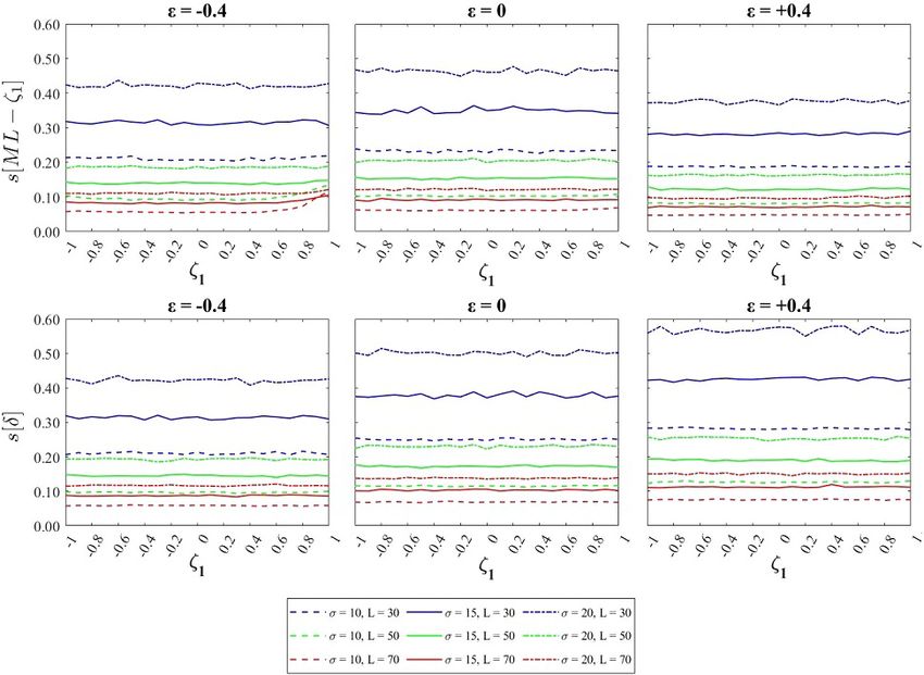
474                            V. Totaro et al.: Numerical investigation on the power of parametric and nonparametric tests

Salas and Obeysekera (2014) provided a detailed report re-               considered nonstationary; otherwise, the variables are “iid”
garding relationships between stationary and nonstationary               (independent, identically distributed) and the model is a sta-
EWT values within a parametric approach for the assessment               tionary one (Montanari and Koutsoyiannis, 2014; Serinaldi
of nonstationary conditions. In such a framework, a strong               and Kilsby, 2015).
relevance is given to statistical tools for detecting changes in            From this perspective, the detection of nonstationarity may
non-normally distributed time series (Kundewicz and Rob-                 exploit (besides traditional statistical tests) well-known prop-
son, 2004).                                                              erties of model selection tools. Even in this case, several mea-
    To date, the vast majority of research regarding climate             sures and criteria are available for selecting a best-fit model,
change and the detection of nonstationary conditions has                 such as the Akaike information criterion (AIC; Akaike,
been developed using nonparametric approaches. One of the                1974), the Bayesian information criterion (BIC; Schwarz,
most commonly used nonparametric measures of trend is                    1978), and the likelihood ratio test (LR; Coles, 2001); the
Sen’s slope (Gocic and Trajkovic, 2013); however, a wide                 latter is suitable when dealing with nested models.
array of nonparametric tests for detecting nonstationarity is               The purpose of this paper is to provide further insights into
available (e.g., Kundewicz and Robson, 2004). Statistical                the use of parametric and nonparametric approaches in the
tests include the Mann–Kendall (MK; Mann, 1945; Kendall,                 framework of extreme event frequency analysis under non-
1975) and Spearman (Lehmann, 1975) tests for detecting                   stationary conditions. The comparison between those differ-
trends, and the Pettitt (Pettitt, 1979) and CUSUM (Smadi and             ent approaches is not straightforward. Nonparametric tests
Zghoul, 2006) tests for change point detection. All of these             do not require knowledge of the parent distribution, and their
tests are based on a specific null hypothesis and have to be             properties strongly rely on the choice of the null hypothe-
performed for an assigned significance level. Nonparametric              sis. Parametric methods for model selection, in comparison,
tests are usually preferred over parametric tests as they are            require the selection of the parent distribution and the esti-
distribution-free and do not require knowledge of the parent             mation of its parameters, but are not necessarily associated
distribution. They are traditionally considered more suitable            with a specific null hypothesis. Nevertheless, in both cases,
for the frequency analysis of extreme events with respect to             the evaluation of the rejection threshold is usually based on
parametric tests because they are less sensitive to the pres-            a statistical measure of trend that, under the null hypothesis
ence of outliers (Wang et al., 2005).                                    of stationarity, follows a specific distribution (e.g., the Gaus-
    In contrast, the use of null hypothesis significance tests           sianity of the Kendall statistic for the MK nonparametric test,
for trend detection has raised concerns and severe criticisms            and the χ 2 distribution of deviance statistic for the LR para-
in a wide range of scientific fields for many years (e.g., Co-           metric test).
hen, 1994), as outlined by Vogel et al. (2013). Serinaldi et                Considering the pros and cons of the different approaches,
al. (2018) provided an extensive critical review focusing on             we believe that specific remarks should be made about the
logical flaws and misinterpretations often related to their mis-         use of parametric and nonparametric methods for the analysis
use.                                                                     of extreme event series. For this purpose, we set up a numer-
    In general, the use of statistical tests involves different er-      ical experiment to compare the performance of (1) the MK
rors, such as type I error (rejecting the null hypothesis when it        as a nonparametric test for trend detection, (2) the LR para-
is true) and type II error (accepting the null hypothesis when           metric test for model selection, and (3) the AICR paramet-
it is false). The latter is related to the test power, i.e., the prob-   ric test, as defined in Sect. 2.3. In particular, the AICR is a
ability of rejecting the null hypothesis when it is false; how-          measure for model selection, based on the AIC, whose distri-
ever, as recognized by a few authors (e.g., Milly et al., 2015;          bution was numerically evaluated, under the null hypothesis
Beven, 2016), the importance of the power has been largely               of a stationary process, for comparison purposes with other
overlooked in Earth system science fields. Strong attention              tests.
has always been paid to the level of significance (i.e., type I             We aim to provide (i) a comparison of test power be-
error), although, as pointed out by Vogel et al. (2013), “a              tween the MK, LR, and AICR ; (ii) a sensitivity analysis of
type II error in the context of an infrastructure decision im-           test power to parameters of a known parent distribution used
plies under-preparedness, which is often an error much more              to generate sample data; and (iii) an analysis of the influ-
costly to society than the type I error (over-preparedness)”.            ence of the sample size on the test power and the significance
    Moreover, as already proven by Yue et al. (2002a), the               level.
power of the Mann–Kendall test, despite its nonparametric                   We conducted the analysis using Monte Carlo techniques;
structure, actually shows a strong dependence on the type                this entailed generating samples from parent populations as-
and parametrization of the parent distribution.                          suming one of the most popular extreme event distributions,
    Using a parametric approach, the estimation of quantiles             the generalized extreme value (GEV; Jenkinson, 1955), with
of an extreme event distribution requires the search for the             a linear (and without any) trend in the position parameter.
underlying distribution and for time-dependant hydrological              From the samples generated, we numerically evaluated the
variables. If variables are time-dependent, they are “i/nid”             power and significance level of tests for trend detection, us-
(independent/non-identically distributed) and the model is               ing the MK, LR, and AICR tests. For the latter, we also

Hydrol. Earth Syst. Sci., 24, 473–488, 2020                                             www.hydrol-earth-syst-sci.net/24/473/2020/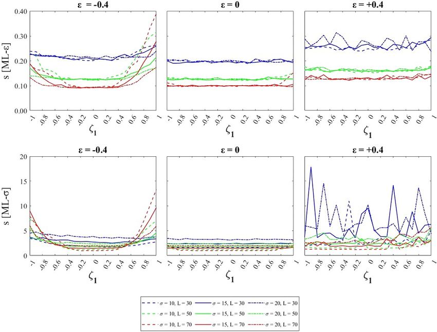
V. Totaro et al.: Numerical investigation on the power of parametric and nonparametric tests 475
checked the option of using the modified version of AIC, re- which follows a standard normal distribution. Using this ap-
ferred to as AICc , suggested by Sugiura (1978) for smaller proach, it is simple to evaluate the p value and compare it
samples. with an assigned level of significance or, equivalently, to cal-
Considering that parametric methods involve the estima- culate the Zα threshold value and compare it with Z, where
tion of the parent distribution parameters, we also analyzed Zα is the (1 − α) quantile of a standard normal distribution.
the efficiency of the maximum likelihood (ML) estimator by Yue et al. (2002b) observed that autocorrelation in time
comparing the sample variability of the ML estimate of trend series can influence the ability of the MK test to detect
with the nonparametric Sen’s slope. Furthermore, we scoped trends. To avoid this problem, a correct approach with respect
the sample variability of the GEV parameters in the station- to trend analysis should contemplate a preliminary check
ary and nonstationary cases. for autocorrelation and, if necessary, the application of pre-
whitening procedures.
A nonparametric tool for a reliable estimation of a trend in
2 Methodological framework a time series with N pairs of data is the Sen’s slope estima-
tor (Sen, 1968), which is defined as the median of the set of
This section is divided into five parts. Sect. 2.1, 2.2, and
slopes δj :
2.3 report the main characteristics of the MK, LR, and AICR
tests, respectively. In Sect. 2.4, the probabilistic model used zi − zk
δj = , j = 1, . . ., N, (2)
for sample data generation, based on the use of the GEV i −k
distribution, is described in the stationary and nonstationary
where i > k.
cases. Finally, Sect. 2.5 outlines the procedure for the numer-
ical evaluation of the tests’ power and significance level. 2.2 Likelihood ratio test
2.1 The Mann–Kendall test The likelihood ratio statistical test allows for the comparison
of two candidate models. As its name suggests, it is based on
Hydrological time series are often composed by non-
the evaluation of the likelihood function of different models.
normally independent realizations of phenomena, and this
The LR test has been used multiple times (Tramblay et
characteristic makes the use of nonparametric trend tests
al., 2013; Cheng et al., 2014; Yilmaz et al., 2014) to select
very attractive (Kundzewicz and Robson, 2004). The Mann–
between stationary and nonstationary models in the context
Kendall test is a widely used rank-based tool for detecting
of nested models. Given a stationary model characterized by
monotonic, and not necessarily linear, trends. Given a ran-
a parameter set θst and a nonstationary model, with parameter
dom variable z, and assigned a sample of L independent data
set θns , if l(θ̂st ) and l(θ̂ns ) are their respective maximized log
z = (z1 , . . . , zL ), the Kendall S statistic (Kendall, 1975) can
likelihoods, the likelihood ratio test can be defined using the
be defined as follows:
deviance statistic
L−1
X L
X h i
D = 2 l θ̂ns − l θ̂st . (3)
S= sgn zj − zi , (1)
i=1 j =i+1
D is (for large L) approximately χm2 distributed, with m =
where “sgn” is the sign function. dim(θns ) − dim(θst ) degrees of freedom. The null hypothesis
The null hypothesis of this test is the absence of any statis- of stationarity is rejected if D > Cα , where Cα is the (1 −
tically significant trend in the sample, whereas the presence α) quantile of the χm2 distribution (Coles, 2001).
of a trend represents an alternative hypothesis. Yilmaz and Besides the analysis of power, we also checked (in
Perera (2014) reported that serial dependence can lead to a Sect. 3.3) the approximation D ∼ χm2 as a function of the
more frequent rejection of the null hypothesis. For L ≥ 8, sample size L for the evaluation of the level of significance.
Mann (1945) reported that Eq. (1) is approximatively a nor-
mal variable with a zero mean and variance which, in the 2.3 Akaike information criterion ratio test
presence of tm ties of length m, can be expressed as
n
Information criteria are useful tools for model selection. It
is reasonable to retain that the Akaike information criterion
P
L(L − 1)(2L + 5) − tm m(m − 1)(2m + 5)
V =
m=1
. (AIC; Akaike, 1974) is the most famous among these tools.
18 Based on the Kullback–Leibler discrepancy measure, if θ is
In practice, the Mann–Kendall test is performed using the the parameter set of a k-dimensional model (k = dim(θ )),
Z statistic AIC is defined as
AIC = −2l(θ̂ ) + 2k. (4)
S−1
√V (S)
S>0
Z= 0 S=0, The model that best fits the data has the lowest value of the
√S+1
S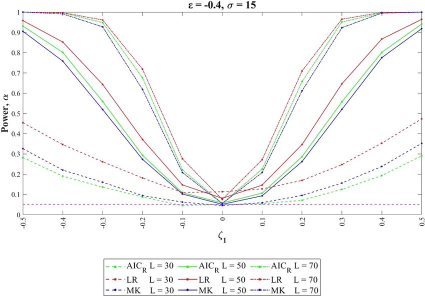
476 V. Totaro et al.: Numerical investigation on the power of parametric and nonparametric tests
proportional to the number of model parameters allows one 2.4 The GEV parent distribution
to account for the increase of the estimator variance as the
number of model parameters increases. The cumulative distribution function of the generalized ex-
Sugiura (1978) observed that the AIC can lead to mislead- treme value (GEV) distribution (Jenkinson, 1955) can be ex-
ing results for small samples; thus, he proposed a new mea- pressed as follows:
sure for the AIC:
h i−1/ε
exp − 1 + ε z−ζ
ε 6= 0
σ
2k(k + 1) F (z, θst ) = n h io σ > 0, (7)
AICc = −2l(θ̂ ) + , (5) exp − exp − z−ζ
ε=0
L−k−1 σ
where ζ , σ , and ε are known as the position, scale, and shape
where a second-order bias correction is introduced. Burn-
parameters, respectively; θst = [ζ , σ , ε] is a general and com-
ham and Anderson (2004) suggested only using this version
prehensive way to express the parameter set in the station-
when L/kmax < 40, with kmax being the maximum number
ary case. The flexibility of the GEV, which accounts for the
of parameters between the models compared. However, for
Gumbel, Fréchet, and Weibull distributions as special cases
larger L, AICc converges to AIC. For a quantitative compar-
(for ε = 0, ε > 0 and ε < 0 respectively) makes it eligible for
ison between the AIC and AICc in the extreme value station-
a more general discussion about the implications of nonsta-
ary model selection framework, the reader is referred to Laio
tionarity.
et al. (2009).
Traditional extreme value distributions can be used in a
In order to select between stationary and nonstationary
nonstationary framework, modeling their parameters as func-
candidate models, we use the ratio
tion of time or other covariates (Coles, 2001), producing
AICns θst −→ θns = [ζt , σt , εt ].
AICR = , (6) In this study, only a deterministic linear dependence on
AICst
the time t of the position parameter ζ has been introduced,
where the subscripts indicate the AIC value obtained for a leading Eq. (7) to be expressed as follows:
stationary (st) and a nonstationary (ns) model, both fitted h i−1/ε
with maximum likelihood to the same data series. exp − 1 + ε z−ζt
ε 6= 0
σ
Considering that the better fitting model has a lower AIC, F (z, θns ) = n h io σ >0 (8)
exp − exp − z−ζt
ε=0
if the time series arises from a nonstationary process, the σ
AICR should be less than 1; the opposite is true if the pro- with
cess is stationary.
ζt = ζ0 + ζ1 t (9)
In order to provide a rigorous comparison between the use
of the MK, LR, and AICR , we evaluated the AICR,α thresh- and θns = [ζ0 , ζ1 , σ , ε].
old value corresponding to the significance level α using nu- It is important to note that Eq. (8) is a more general way of
merical experiments. defining the GEV and has the property of degenerating into
More in detail, we adopted the following procedure: Eq. (7) for ζ1 = 0; in other words, Eq. (7) represents a nested
model of Eq. (8) which would confirm the suitability of the
1. N = 10 000 samples are generated from a stationary likelihood ratio test for model selection.
GEV parent distribution, with known parameters; According to Muraleedharan et al. (2010), the first three
2. for each of these samples the AICR is evaluated by fit- moments of the GEV distribution are as follows:
σ
ting the stationary and nonstationary GEV models de- mean = ζ + (g1 − 1) ε 6 = 0, ε < 1, (10)
scribed in Sect. 2.4, thus providing its empirical distri- ε
bution (see probability density function, pdf, in Fig. 1); σ2 1
variance = 2 g2 − g12 ε 6 = 0, ε < , and (11)
ε 2
3. exploiting the empirical distribution of AICR , the
g3 − 3g2 g1 + 2g13 1
threshold associated with a significance level of α = skewness = sgn(ε) · 3/2 ε 6 = 0, ε < 3 . (12)
g2 − g 2
0.05 is numerically evaluated. This value, AICR,α , rep- 1
resents the threshold for rejecting the null hypothesis of Here, gk = 0(1 − kε), with k ∈ Z + and 0(·), is the gamma
stationarity (which in these generations is true) in 5 % function. It is worth noting that, following Eqs. (10)–(12), the
of the synthetic samples. trend in the position parameter only affects the mean, while
This procedure was applied both for the AIC and AICc . The the variance and skewness remain constant.
experiment was repeated for a few selected sets of the GEV In this work, we used the maximum likelihood
parameters, including different trend values, and different method (ML) to estimate the GEV parameters from sample
sample lengths, as detailed in Sect. 3. data. The ML allows one to treat ζ1 as an independent param-
eter, as well as ζ0 , σ and ε. For this purpose, we exploited the
“extRemes” R package (Gilleland and Katz, 2016).
Hydrol. Earth Syst. Sci., 24, 473–488, 2020 www.hydrol-earth-syst-sci.net/24/473/2020/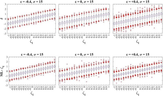
V. Totaro et al.: Numerical investigation on the power of parametric and nonparametric tests                                        477

Figure 1. An empirical distribution of AICR and the rejection threshold AICR,α of the null hypothesis (stationary GEV parent).

2.5   Numerical evaluation of test power and significance              The same procedure, with N = 10 000, was used in order to
      level                                                            check the actual significance level of the test, which is the
                                                                       probability of type I error, i.e., the probability of rejecting
The power of a test is related to the type II error and is the         the null hypothesis of stationarity when it is true. The task
probability of correctly rejecting the null hypothesis when            was performed by following the abovementioned steps 1 to 3
it is false. In particular, defining α (level of significance), the    while replacing θns with θst in step 1); in such a case, the
probability of a type I error, and β, the probability of a type II     rejection rate Nrej /N represents the actual level of signifi-
error, we have a power value of 1 − β. The maximum value               cance α.
of power is 1, which correspond to β = 0, i.e., no probabil-              We used a reduced number of generations (N = 2000) for
ity of a type II error. In most applications, the conventional         the evaluation of power as a good compromise between the
values are α = 0.05 and β = 0.2, meaning that a 1-to-4 trade-          quality of the results and computational time. N = 2000 was
off between α and β is accepted. Thus, in our experiment we            also used by Yue et al. (2002a).
always assumed a significance level of 0.05, and, for the fol-
lowing description of results and discussion, we considered
a power level of less than 0.8 to be too low and, hence, unac-         3   Sensitivity analysis, results, and discussion
ceptable. In Sect. 4, we report further considerations regard-
ing this choice. For each of the tests described in Sect. 2.1,         A comparative evaluation of the tests’ performance was car-
2.2, and 2.3, the power was numerically evaluated according            ried out for different GEV parameter sets θns , considering
to the following procedure:                                            three values of ε (−0.4, 0, and 0.4) and three values of σ
                                                                       (10, 15, and 20). The position parameter was always kept
  1. N = 2000 Monte Carlo synthetic series, each of                    constant and equal to ζ0 = 40. Then, for any possible pair
     length L, are generated using the nonstationary GEV               of σ and ε values, we considered ζ1 ranging from −1 to 1
     in Eqs. (8) and (9) as a parent distribution with a fixed         with a step size of 0.1. Such a range of parameters repre-
     parameter set θns = [ζ0 , ζ1 , σ , ε] with ζ1 6 = 0.              sents a wide domain in the hydrologically feasible parame-
  2. The threshold AICR,α associated with a significance               ter space of annual maximum daily rainfall. Upper-bounded
     level of α = 0.05 is numerically evaluated, as described          (ε = −0.4), EV1 (ε = 0), and heavy-tailed (ε = +0.4) cases
     in Sect. 2.3, using the corresponding parameter set θst =         are included. Moreover, for each of these parameter sets θns ,
     [ζ0 , σ , ε] of the GEV parent distribution.                      N samples of different sizes (30, 50, and 70) were generated.
                                                                          For a clear exposition of the results, this section is divided
  3. From these synthetic series, the power of the test is es-         into four subsections. In Sect. 3.1, we focus on the oppor-
     timated as                                                        tunity to use the AIC or AICc for the evaluation of AICR ;
                         Nrej                                          in Sect. 3.2, the comparison of test power and its sensitivity
      rejection rate =        ,                                        analysis to the parent distribution parameters and the sam-
                          N
                                                                       ple size is shown; in Sect. 3.3, the evaluation of the level of
      where Nrej is the number of series for which the null
                                                                       significance for all tests and, in particular, the validity of the
      hypothesis is rejected, as in Yue et al. (2002a).
                                                                       χ 2 approximation for the D statistic is discussed; and finally

www.hydrol-earth-syst-sci.net/24/473/2020/                                              Hydrol. Earth Syst. Sci., 24, 473–488, 2020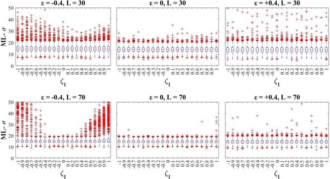
478 V. Totaro et al.: Numerical investigation on the power of parametric and nonparametric tests
in Sect. 3.4, the numerical investigation of the sample vari- trend coefficient for one set of parameter values and different
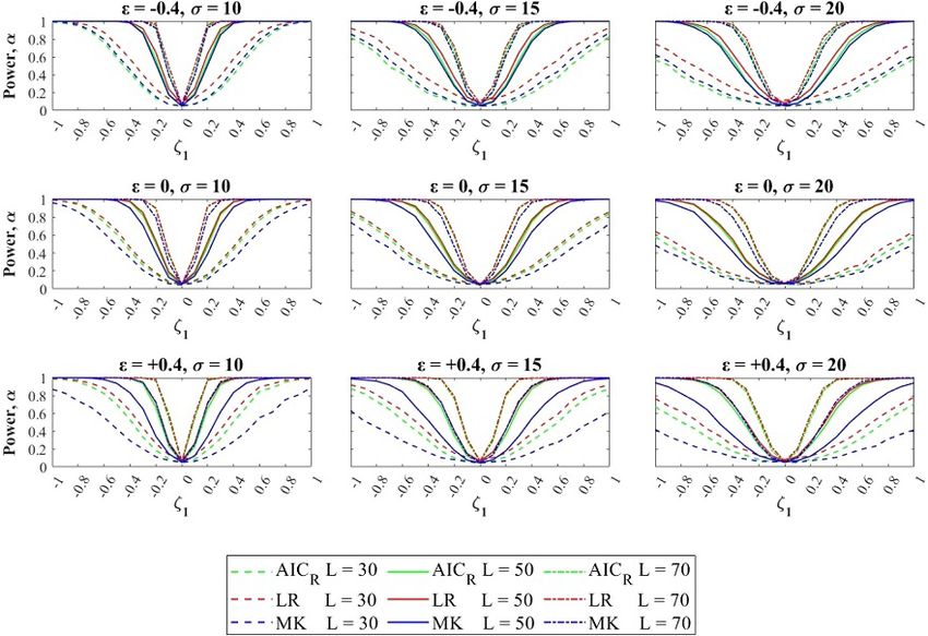
ability of the parameters is reported. sample sizes. In all panels, the test power strongly depends
on the trend coefficient and sample size. This dependence is
3.1 Evaluation of AICR , with the AIC and AICc also affected by the parent parameter values. In all cases, the
power reaches 1 for a strong trend and approaches 0.05 (the
Considering the nonstationary GEV four-parameter model, chosen level of significance) for a weak trend (ζ1 close to 0).
in order to satisfy the relation L/kmax < 40 suggested by In all combinations of the shape and scale parameters (and
Burnham and Anderson (2004), a time series with a record especially for short samples) for a wide range of trend val-
length no less than 160 should be available. Following this ues, the power exhibits values well below the conventional
simple reasoning, the AIC should be considered not to be value of 0.8. The curves’ slope between 0.05 and 1 is sharp
applicable to any annual maximum series showing a chang- for long samples and gentle for short samples. It also depends
ing point between the 1970s and 1980s (e.g., Kiely, 1999). on the parameter set, with slopes generally being gentler for
In our numerical experiment, the second-order bias correc- higher values of the scale (σ ) and shape (ε) parameters of
tion of Sugiura (1978) should always be used, as we have the parent distribution. A significant difference in the power
L/kmax = 70/4 = 17.5 for the nonstationary GEV for a max- between the MK, LR, and AICR tests is observable when the
imum sample length of L = 70. Nevertheless, we checked if sample size is smaller and even more so when the parent dis-
using the AIC or AICc may affect results. For this purpose, tribution is heavy-tailed (ε = +0.4).
we evaluated the percentage differences between the power In particular, for ε = 0, −0.4 and L = 50, 70, it is possi-
of the AICR obtained by means of the AIC and AICc from ble to report a slightly larger power of LR with respect to the
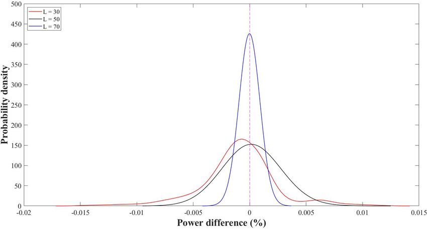
synthetic series. In Fig. 2, the empirical probability density AICR and MK, but values are very close to each other. How-
functions of such percentage differences, grouped according ever, the reciprocal position of MK and AICR power curves
to sample length, are plotted for generations with ε = 0.4 and is interesting; in fact, the AICR power is always larger than
different values of σ . It is interesting to note that the error that of the MK, except when ε = −0.4, for all values of the
distribution only shows a regular and unbiased bell-shaped scale parameter.
distribution for L = 70. We then observe a small negative A higher difference is found for a heavy-tailed parent dis-
bias (about −0.02 %) for L = 50, while a bias of −0.08 with tribution (ε = +0.4). While LR still has the largest power
a multi-peak and negatively skewed pdf is noted for L = 30. value, the difference with respect to AI CR remains small
The latter pdf also has a higher variance than the others. The and the MK power value almost always collapses to values
purpose of this figure is to show that the difference between smaller than 0.5.
the power obtained with the AIC and the power obtained with The practical consequences of such patterns are very im-
the AICc is negligible. Different peaks in one curve (L = 30) portant and are discussed in Sect. 4.
can be explained by the merging of sample errors obtained
for different values of σ . Similar results were obtained for all 3.3 Sensitivity and evaluation of the actual significance
values of ε, which always provided very low differences and level
allow for the conclusion to be reached that the use of the AIC
or AICc does not significantly affect the power of AICR for We evaluated the threshold values (corresponding to a signif-
the cases examined. This follows the combined effect of the icance level of 0.05) for accepting/rejecting the null hypothe-
sample size (whose minimum value considered here is 30) sis of stationarity according to the methodologies recalled in
and the limited difference in the number of parameters in the Sect. 2.1 and 2.2 for the MK and LR tests and introduced in
selected models. In the following, we will refer to and show Sect. 2.3 for AICR . Based on these thresholds, we exploited
only the plots obtained for the AICR in Eq. (6) with the AIC the generation of series from a stationary model (ζ1 = 0) in
evaluated as in Eq. (4). order to numerically evaluate the rate of rejection of the null
hypothesis, i.e., the actual significance level of the tests con-
3.2 Dependence of the power on the parent distribution sidered in the numerical experiment, following the procedure
parameters and sample size described in Sect. 2.5.
Table 1 shows the numerical values of the actual level of
The effect of the parent distribution parameters and the sam- significance, obtained numerically, to be compared with the
ple size on the numerical evaluation of the power and sig- theoretical value of 0.05 for all of the sets of parameters and
nificance level of the MK, LR, and AICR tests for different sample sizes considered. Among the three measures for trend
values of ε, σ , and ζ1 is shown in Fig. 3. The curves repre- detection, the LR shows the worst performance. The results
sent both the significance level, which is shown for ζ1 = 0 in Table 1 show that the rejection rate of the (true) null hy-
(true parent is the stationary GEV), and the power, which is pothesis is systematically higher than it should be, and it
shown for all other values ζ1 6 = 0 (true parent is the nonsta- is also dependent on parent parameter values. This effect is
tionary GEV). Each panel in Fig. 3 shows the dependence of exalted when the parent distribution has an upper boundary
the power and significance level of MK, LR and AICR on the (ε = −0.4) and for shorter series (L = 30). In practice, this
Hydrol. Earth Syst. Sci., 24, 473–488, 2020 www.hydrol-earth-syst-sci.net/24/473/2020/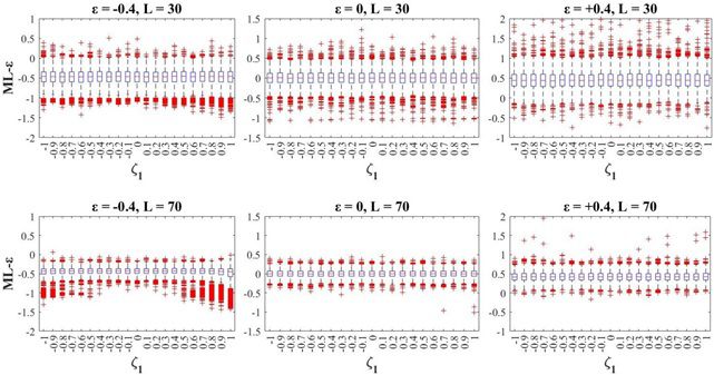
V. Totaro et al.: Numerical investigation on the power of parametric and nonparametric tests                                     479

Figure 2. Distributions of the differences between the power of AICR evaluated with the AIC and AICc for ε = 0.4.

Figure 3. Dependence of test power on the trend coefficient, sample size, scale, and shape of the parent parameters.

implies that when using the LR test, as described in Sect. 2.2,         obtained for the AICR , whose rejection threshold is numeri-
there is a higher probability of rejecting the null hypothesis          cally evaluated.
of stationarity (if it is true) than expected or designed.                 The plot in Fig. 4 is displayed in order to focus on the
   Conversely, the performance of MK with respect to the de-            actual value of the level of significance and, in particular,
signed level of significance is less biased and is independent          on the LR approximation D ∼ χm2 as a function of the sam-
of the parameter set. Similar good performance is trivially             ple length L. The difference between the theoretical and nu-

www.hydrol-earth-syst-sci.net/24/473/2020/                                               Hydrol. Earth Syst. Sci., 24, 473–488, 2020
480                            V. Totaro et al.: Numerical investigation on the power of parametric and nonparametric tests

Table 1. The actual level of significance of the tests for different sample sizes, scales, and shapes of the parent parameters.

                                    ε = −0.4                              ε=0                               ε = +0.4
                          σ = 10     σ = 15     σ = 20        σ = 10     σ = 15     σ = 20         σ = 10     σ = 15    σ = 20
                L = 30
                MK         0.048      0.047      0.047         0.047      0.050      0.050         0.046      0.049      0.048
                AICR       0.050      0.046      0.052         0.051      0.052      0.045         0.052      0.054      0.051
                LR         0.104      0.103      0.115         0.061      0.064      0.060         0.084      0.081      0.083
                L = 50
                MK         0.050      0.047      0.046         0.044      0.047      0.050         0.049      0.044      0.048
                AICR       0.053      0.053      0.046         0.051      0.051      0.057         0.050      0.050      0.053
                LR         0.079      0.078      0.074         0.060      0.063      0.063         0.070      0.069      0.070
                L = 70
                MK         0.050      0.052      0.054         0.052      0.051      0.047         0.049      0.048      0.046
                AICR       0.047      0.051      0.051         0.058      0.058      0.052         0.050      0.054      0.051
                LR         0.069      0.069      0.073         0.063      0.065      0.058         0.062      0.062      0.063

Figure 4. Enlargement of the power test curves in the case (σ = 15, ε = −0.4), with focus on the actual level of significance (ζ1 = 0).

merical values of the significance level is represented by the             as a consequence of the significance level overestimation,
distance between the bottom value of the curve (obtained                   meaning that the LR test power is also overestimated due
for ζ1 = 0, i.e., the stationary GEV model) and the chosen                 to the approximation D ∼ χm2 . These results suggest the use
level of significance 0.05, represented by the horizontal dot-             of a numerical procedure for the LR test (such as that intro-
ted line. In particular, in Fig. 4, results for the parameter set          duced for AICR in Sect. 2.3) for evaluating the D distribution
(σ = 15, ε = −0.4) show that the actual rate of rejection is               and the rejection threshold.
always higher than the theoretical one and changes signifi-                   Other considerations can be made regarding the use of
cantly with the sample size; this means that the χm2 approx-               AICR . As explained in Sect. 2.3, we empirically evaluated
imation leads to a significant underestimation of the rejec-               the AICR,α threshold value using numerical generations with
tion threshold of the D statistic. Moreover, it seems that the             a significance level 0.05 for each of the parameter sets and
LR power curves (in red) are shifted toward higher values                  sample sizes considered. Similar results were obtained us-

Hydrol. Earth Syst. Sci., 24, 473–488, 2020                                                  www.hydrol-earth-syst-sci.net/24/473/2020/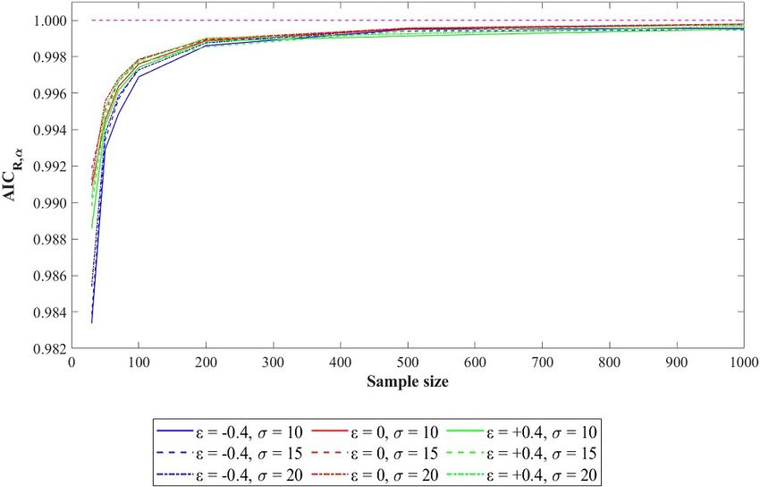
V. Totaro et al.: Numerical investigation on the power of parametric and nonparametric tests                                        481

Table 2. Actual level of significance of the AICR test for AICR,α = 1.

                                   ε = −0.4                              ε=0                               ε = +0.4
                          σ = 10    σ = 15     σ = 20        σ = 10      σ = 15     σ = 20        σ = 10   σ = 15     σ = 20
               L = 30     0.246      0.254     0.261         0.188       0.191       0.181         0.220    0.221     0.215
               L = 50     0.213      0.209     0.206         0.171       0.175       0.170         0.188    0.207     0.195
               L = 70     0.192      0.192     0.201         0.168       0.169       0.173         0.184    0.204     0.184

Figure 5. AICR,α thresholds for different parameter sets vs. sample size.

ing the AICc , which are not shown for brevity. We found a               an unknown significance level that is dependent on the par-
significant dependence of AICR,α on the sample size. Fig-                ent distribution and sample size. In order to highlight this
ure 5 shows the AICR,α curves obtained for each of the pa-               point, we evaluated the significance level α corresponding to
rameter sets vs. sample size. It is also worth noting that all           AICR,α = 1, following the procedure described in Sect. 2.5,
curves asymptotically trend to 1 as L increases. This prop-              by generating N = 10 000 synthetic series (from a station-
erty is due to the structure of the AIC and the peculiarity              ary model) for any parameter set and sample length. The re-
of the nested models used in this paper: while using a sam-              sults, provided in Table 2, show that α ranges between 0.16
ple generated with weak nonstationarity (i.e., when ζ1 → 0               and 0.26 in the explored GEV parameter domain and mainly
in Eq. 9), the maximum likelihood of the model shown in                  depends on the sample length and the shape parameter of the
Eq. 7, l(θ̂st ), tends toward l(θ̂ns ) of the model shown in Eq. 8,      parent distribution.
leaving only the bias correction (2k in equation 4) to discrim-
inate between competing AIC values in model selection ap-                3.4      Sample variability of parent distribution
plications. As a consequence, the AICR,α should always be                         parameters
lower than 1; however, when increasing the sample size, both
the likelihood terms −2l(θ̂st ) and −2l(θ̂ns ) in Eq. (4) will           In our opinion, the results shown above, with respect to the
also increase, pushing AICR toward the limit 1. Conversely,              performance of parametric and nonparametric tests, are quite
Fig. 5 shows that the threshold value AICR,α is significantly            surprising and important. It is proved that the preference
smaller than 1 up to L values well beyond the length usually             widely accorded to nonparametric tests, due to the fact that
available in this kind of analysis. Hence, the numerical evalu-          their statistics are allegedly independent from the parent dis-
ation of the threshold has to be considered as a required task           tribution, is not well founded. Conversely, the use of para-
in order to provide an assigned significance level to model              metric procedures raises the problem of correctly estimat-
selection. In contrast, the simple adoption of the selection             ing the parent distribution and, for the purpose of this pa-
criteria AICR < 1 (i.e., AICR,α = 1) would correspond to                 per, its parameters. Moreover, as the trend coefficient ζ1 is a
                                                                         parameter of the parent distribution under nonstationary con-

www.hydrol-earth-syst-sci.net/24/473/2020/                                                   Hydrol. Earth Syst. Sci., 24, 473–488, 2020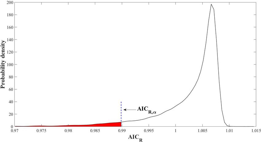
482                           V. Totaro et al.: Numerical investigation on the power of parametric and nonparametric tests

Figure 6. Sample variability of ML-ζ1 and δ vs. the trend coefficient ζ1 .

ditions, the proposed parametric approach provides a max-                    the range of trend values that may result from a local evalua-
imum likelihood-based estimation of the same trend coeffi-                   tion. Similar results, characterized by smaller sample vari-
cient, which is hereafter referred to as ML-ζ1 . For a compar-               ability, as shown in Fig. 6, are obtained for L = 50 and
ison with nonparametric approaches, we also evaluated the                    L = 70 and are not shown for brevity.
sample variability of the Sen’s slope measure (δ) of the im-                    Figure 8 shows the sample variability of ML-ε and ML-σ ,
posed linear trend. Furthermore, in order to provide insights                which is still independent of the true ζ1 for values of ε = 0
into these issues, we analyzed the sample variability of the                 and 0.4, whereas for the upper-bounded GEV distributions
maximum likelihood estimates ML-ε and ML-σ (from the                         (ε = −0.4) it shows a significant increase for higher values
same sets of generations exploited above) for different pa-                  of σ and high trend coefficients (|ζ1 | > 0.5). The randomness
rameter sets and sample lengths.                                             of results for L = 30 and σ = [15, 20] is probably due to the
   We evaluated sample variability s[·], as the standard devi-               reduced efficiency of the algorithm that maximizes the log-
ation of the ML estimates of parameter values obtained from                  likelihood function for heavy-tailed distributions.
synthetic series. In the upper panels of Fig. 6, we show s[ML-                  In order to better analyze such patterns, for the scale and
ζ1 ], and in the lower panels, we show the Sen’s slope median                shape parent parameters we also report the distribution of
s[δ]. In both cases, the sample variability of the linear trend is           their empirical ML estimates for different parameter sets
strongly dependent on sample size and independent from the                   vs. the true ζ1 value used in generation. The sample distri-
true ζ1 value in the range examined [−1, 1]. It reaches high                 bution of ML-ε for σ = 15 is shown in Fig. 9 for L = 30
values for short samples and, in such cases, its dependence on               and L = 70. The sample distribution of ML-σ for σ = 15 is
the scale and shape parent parameters is also relevant. The                  shown in Fig. 10 for L = 30 and L = 70. The panels show
ML estimation of the trend coefficient is always more effi-                  that the presence of a strong trend coefficient may produce
cient than Sen’s slope, and this is observed for heavy-tailed                significant loss in the estimator efficiency, which is probably
distributions in particular.                                                 due to deviation from the normal distribution of the sample
   In Fig. 7, we show the empirical distributions of the Sen’s               estimates for long samples. This suggests the need for more
slope δ and ML-ζ1 estimates obtained from samples of size                    robust estimation procedures that provide higher efficiency
L = 30 with a parent distribution characterized by σ = 15                    for estimates of ε and σ in the case of a strong observed trend.
and ε = [−0.4, 0, 0.4], providing visual information about                   It should be highlighted that efficiency in the parameter esti-

Hydrol. Earth Syst. Sci., 24, 473–488, 2020                                                 www.hydrol-earth-syst-sci.net/24/473/2020/
V. Totaro et al.: Numerical investigation on the power of parametric and nonparametric tests                                    483

Figure 7. Empirical distributions of δ and ML-ζ1 evaluated from samples with L = 30 and σ = 15 vs. the trend coefficient ζ1 .

Figure 8. Sample variability of ML-ε and ML-σ vs. the trend coefficient ζ1 .

www.hydrol-earth-syst-sci.net/24/473/2020/                                              Hydrol. Earth Syst. Sci., 24, 473–488, 2020
484                          V. Totaro et al.: Numerical investigation on the power of parametric and nonparametric tests

Figure 9. Empirical distributions of ML-ε evaluated for σ = 15 from samples with L = 30 and L = 70 vs. the trend coefficient ζ1 .

Figure 10. Empirical distributions of ML-σ evaluated for σ = 15 from samples with L = 30 and L = 70 vs. the trend coefficient ζ1 .

mation increases with sample size for ε = [0, 0.4], whereas               Considering the feasibility of the numerical evaluation of
it decreases for both ε and σ in the case of ε = −0.4, where           power, allowed by the parametric approach, we observe that,
the trend of the location parameter implies a shift in time of         while awareness of the crucial role of type II error has been
the distribution upper bound.                                          growing in recent years in the hydrological literature, a com-
                                                                       mon debate would deserve more development about which
                                                                       power values should be considered acceptable. Such an is-
4   Conclusions                                                        sue is much more enhanced in other scientific fields where
                                                                       the experimental design is traditionally required to estimate
The results shown have important practical implications.
                                                                       the appropriate sample size to adequately support results and
The dependence of test power on the parent distribution pa-
                                                                       conclusions. In psychological research, Cohen (1992) pro-
rameters may significantly affect results of both parametric
                                                                       posed 0.8 to be a conventional value of power to be used
and nonparametric tests, including the widely used Mann–
                                                                       with level of significance of 0.05, thus leading to a 4 : 1 ra-
Kendall test.

Hydrol. Earth Syst. Sci., 24, 473–488, 2020                                            www.hydrol-earth-syst-sci.net/24/473/2020/
V. Totaro et al.: Numerical investigation on the power of parametric and nonparametric tests 485 tio between the risk of type II and type I error. The conven- These problems affect both parametric and nonparametric tional value proposed by Cohen (1992) has been taken as a tests (to slightly different degrees). While these considera- reference by thousands of papers in social and behavioral sci- tions are generally applicable to all of the tests considered, ences. In pharmacological and medical research, depending differences also emerge between them. For heavy-tailed par- on the real implications and the nature of the type II error, ent distributions and smaller samples, the MK test power conventional values of power may be as high as 0.999. This decreases more rapidly than for the other tests considered. was the value suggested by Lieber (1990) for testing a treat- Low values of power are already observable for L = 50. The ment for patients’ blood pressure. The author stated, while LR test slightly outperforms the AICR for small sample sizes “guarding against cookbook application of statistical meth- and higher absolute values of the shape parameter. Neverthe- ods”, “it should also be noted that, at times, type II error may less, the higher value of the LR power seems to be overes- be more important to an investigator then type I error”. timated as a consequence of the χm2 approximation for the We believe that, when selecting between stationary and D statistic distribution (see Sect. 3.3). nonstationary models for extreme hydrological event predic- Results also suggest that the theoretical distribution of the tion, a fair comparison between the null and the alternative LR test-statistic based on the null hypothesis of stationarity hypotheses of α = β = 0.05 should be utilized, which pro- may lead to a significant increase in the rejection rate com- vides a power value of 0.95. In our discussion, we consid- pared with the chosen level of significance, i.e., an abnormal ered 0.8 to be a minimum threshold for acceptable power rate of rejection of the null hypothesis when it is true. In this values. case, the use of numerical techniques, based on the imple- For all of the generation sets and tests conducted, under the mentation of synthetic generations performed by exploiting null hypothesis of stationarity, the power has values ranging a known parent distribution, should be preferred. between the chosen significance level (0.05) and 1 for large In light of these results, we conclude that the assessment (and larger) ranges of the trend coefficient. The test power al- of the parent distribution and the choice of the null hypoth- ways collapses to very low values for weak (but climatically esis should be considered as fundamental preliminary tasks important) trend values (e.g., in the case of annual maximum in trend detection on annual maximum series. Therefore, it daily rainfall, ζ1 was equal to 0.2 or 0.3 mm yr−1 ). In the is advisable to make use of parametric tests by numerically presence of a trend, the power is also affected by the scale evaluating both the rejection threshold for the assigned sig- and shape parameters of the GEV parent distribution. This nificance level and the power corresponding to alternative hy- observation can be made with reference to samples of all of potheses. This also requires the development of robust tech- the lengths considered in this paper (from 30 to 70 years of niques for selecting the parent distribution and estimating its observations), but the use of smaller samples significantly re- parameters. To this end, the use of a parametric measure such duces the test power and dramatically extends the range of ζ1 as the AICR , may take different choices for the parent distri- values for which the power is below the conventional value of bution into account and, even more importantly, allow one to 0.8. The use of this sample size is not rare considering that set the null hypothesis differently from the stationary case, significant trends due to anthropic effects are typically inves- based on a priori information. tigated in periods following a changing point often observed The need for robust procedures to assess the parent dis- in the 1980s. tribution and its parameters is also proven by the numer- These results also imply that in spatial fields where the al- ical simulations that we conducted. Sample variability of ternative hypothesis of nonstationarity is true but the parent’s parameters (including the trend coefficient) may increase parameters (including the trend coefficient) and the sample rapidly for series with L values as low as 30 years of the length are variable in space, the rate of rejection of the false annual maxima. Moreover, we observed that, in the case of null hypothesis may be highly variable from site to site and high trends, numerical instability and non-convergence of the power, if left without control, de facto assumes random algorithms may affect the estimation procedure for upper- values in space. In other words, the probability of recog- bounded and heavy-tailed distributions. Nevertheless, the nizing the alternative hypothesis of nonstationarity as true sample variability of the ML trend estimator was always from a single observed sample may unknowingly change (be- found to be smaller than the Sen’s slope sample variability. tween 0.05 and 1) from place to place. For small samples Finally, it is worth noting that the nonparametric Sen’s slope (e.g., L = 30 in our analysis) and heavy-tailed distributions, method, applied to synthetic series, also showed dependence the power is always very low for the entire investigated range on the parent distribution parameters, with sample variability of the trend coefficient. being higher for heavy-tailed distributions. Therefore, considering the high spatial variability of the This analysis shed light on important eventual flaws in the parent distribution parameters and the relatively short pe- at-site analysis of climate change provided by nonparametric riod of reliable and continuous historical observations usu- approaches. Both test power and trend evaluation are affected ally available, a regional assessment of trend nonstationarity by the parent distribution as is also the case for paramet- may suffer from the different probability of the rejection of ric methods. It is not by chance, in our opinion, that many the null hypothesis of stationarity (when it is false). technical studies that have recently been conducted around www.hydrol-earth-syst-sci.net/24/473/2020/ Hydrol. Earth Syst. Sci., 24, 473–488, 2020
486                         V. Totaro et al.: Numerical investigation on the power of parametric and nonparametric tests

the world provide inhomogeneous maps of positive/negative          cobellis et al., 2011; see Rosbjerg et al., 2013 for a more
trends and large areas of stationarity characterized by weak       extensive overview).
trends that are not considered statistically significant.             Hence, we believe that “learning from data” (Sivapalan,
   As already stated, an advantage of using parametric tests       2003), will remain a key task for hydrologists in future years,
and numerical evaluation of the test statistic distribution is     as they face the challenge of consistently identifying both
given by the possibility of assuming a null hypothesis based       deterministic and stochastic components of change (Monta-
on a preliminary assessment of the parent distribution, in-        nari et al., 2013). This involves crucial and interdisciplinary
cluding trend detection via the evaluation of nonstationary        research to develop suitable methodological frameworks for
parameters. This could lead to a regionally homogeneous and        enhancing physical knowledge and data exploitation, in order
controlled assessment of both the significance level and the       to reduce the overall uncertainty of prediction in a changing
power in a fair mutual relationship. With respect to the es-       environment.
timation of the parameters of the parent distribution, results
suggest that at-site analysis may provide highly biased re-
sults. More robust procedures are necessary, such as hier-         Data availability. No data sets were used in this article.
archic estimation procedures (Fiorentino et al., 1987), and
procedures that provide estimates of ε and σ from detrended
series (Strupczewski et al., 2016; Kochanek et al., 2013).         Author contributions. All authors contributed in equal measure to
   As a final remark, concerning real data analysis, in our nu-    all stages of the development and production of this paper.
merical experiment we showed that a weak linear trend in
the mean suffices to reduce power to unacceptable values in
some cases. However, we explored the simplest nonstation-          Competing interests. The authors declare that they have no conflict
                                                                   of interest.
ary working hypothesis by introducing a deterministic linear
dependence of the location parameter of the parent distribu-
tion on time. Obviously, when making inference from real
                                                                   Acknowledgements. The authors thank the three anonymous re-
observed data, other sources of uncertainty may affect sta-        viewers and the editor Giuliano Di Baldassarre, who all helped to
tistical inference (trend, heteroscedasticity, persistence, non-   extend and the improve the paper.
linearity, and so on); moreover, if considering a nonstation-
ary process with underlying deterministic dynamics, the pro-
cess becomes non-ergodic, implying that statistical inference      Financial support. The present investigation was partially carried
from sampled series is not representative of the process’s en-     out with support from the Puglia Region (POR Puglia FESR-
semble properties (Koutsoyiannis and Montanari, 2015).             FSE 2014–2020) through the “T.E.S.A.” – Tecnologie innovative
   As a consequence, when considering a nonstationary              per l’affinamento Economico e Sostenibile delle Acque reflue depu-
stochastic process as being produced by a combination of           rate rivenienti dagli impianti di depurazione di Taranto Bellavista e
a deterministic function and a stationary stochastic process,      Gennarini – project.
other sources of information and deductive arguments should
be exploited in order to identify the physical mechanism un-
derlying such relationships. Also, in this case observed time      Review statement. This paper was edited by Giuliano Di Baldas-
series have a crucial role in the calibration and validation of    sarre and reviewed by three anonymous referees.
deterministic modeling; in other words, they are important
for confirming or disproving the model hypotheses.
   In the field of frequency analysis of extreme hydrological
events, considering the high spatial variability of the sample     References
length, the trend coefficient, the scale, and the shape parame-
ters, among others, physically based probability distributions     Akaike, H.: A new look at the statistical model iden-
could be further developed and exploited for the selection           tification, IEEE T. Automat. Control, 19, 716–723,
and assessment of the parent distribution in the context of          https://doi.org/10.1109/TAC.1974.1100705, 1974.
nonstationarity and change detection. The physically based         Beven, K.: Facets of uncertainty: Epistemic uncertainty,
probability distributions we refer to are (i) those arising from     non-stationarity,    likelihood,  hypothesis     testing,  and
                                                                     communication, Hydrolog. Sci. J., 61, 1652–1665,
stochastic compound processes introduced by Todorovic and
                                                                     https://doi.org/10.1080/02626667.2015.1031761, 2016.
Zelenhasic (1970), which also include the GEV (see Madsen
                                                                   Burnham, K. P. and Anderson, D. R.: Model selection and multi-
et al., 1997) and the TCEV (Rossi et al., 1984), and (ii) the        model inference, Springer, New York, 2004.
theoretically derived distributions following Eagleson (1972)      Cheng, L., AghaKouchak, A., Gilleland, E., and Katz, R. W.:
whose parameters are provided by clear physical meaning              Non-stationary extreme value analysis in a changing climate,
and are usually estimated with the support of exogenous in-          Climatic Change, 127, 353–369, https://doi.org/10.1007/s10584-
formation in regional methods (e.g., Gioia et al., 2008; Ia-         014-1254-5, 2014.

Hydrol. Earth Syst. Sci., 24, 473–488, 2020                                        www.hydrol-earth-syst-sci.net/24/473/2020/
V. Totaro et al.: Numerical investigation on the power of parametric and nonparametric tests 487 Chow, V. T. (Ed.): Statistical and probability analysis of hydrologic Shiryayev, A. N., Kluwer, Dordrecht, the Netherlands, 62– data, in: Handbook of applied hydrology, McGraw-Hill, New 108, https://doi.org/10.1007/BF01457949, 1931. York, 8.1–8.97, 1964. Koutsoyiannis, D. and Montanari A.: Negligent killing of scientific Cohen, J.: A power primer, Psycholog. Bull., 112, 155–159, 1992. concepts: the stationarity case, Hydrolog. Sci. J., 60, 1174–1183, Cohen, J.: The Earth Is Round (p < .05), Am. Psychol., 49, 997– https://doi.org/10.1080/02626667.2014.959959, 2015. 1003, 1994. Kundzewicz, Z. W. and Robson, A. J.: Change detection in hydro- Coles, S.: An Introduction to Statistical Modeling of Extreme Val- logical records – a review of the methodology, Hydrolog. Sci. J., ues, Springer, London, 2001. 49, 7–19, https://doi.org/10.1623/hysj.49.1.7.53993, 2004. Cooley, D.: Return Periods and Return Levels Under Climate Laio, F., Baldassarre, G. D., and Montanari, A.: Model Change, in: Extremes in a Changing Climate, edited by: AghaK- selection techniques for the frequency analysis of hy- ouchak, A., Easterling, D., Hsu, K., Schubert, S., and Sorooshian, drological extremes, Water Resour. Res., 45, W07416, S., Springer, Dordrecht, 97–113, https://doi.org/10.1007/978-94- https://doi.org/10.1029/2007wr006666, 2009. 007-4479-0_4, 2013. Lehmann, E. L.: Nonparametrics, Statistical Methods Based on Du, T., Xiong, L., Xu, C. Y., Gippel, C. J., Guo, S., and Ranks, Holden-Day, Oxford, England, 1975 Liu, P.: Return period and risk analysis of nonstationary low- Lieber, R. L.: Statistical significance and statistical power flow series under climate change, J. Hydrol., 527, 234–250, in hypothesis testing, J. Orthop. Res., 8, 304–309, https://doi.org/10.1016/j.jhydrol.2015.04.041, 2015. https://doi.org/10.1002/jor.1100080221, 1990. Eagleson, P. S.: Dynamics of flood frequency, Water Resour. Res., Madsen, H., Rasmussen, P., and Rosbjerg, D.: Comparison of an- 8, 878–898, https://doi.org/10.1029/WR008i004p00878, 1972. nual maximum series and partial duration series for modelling Fiorentino, M., Gabriele, S., Rossi, F., and Versace, P.: Hierarchi- exteme hydrological events: 1. At-site modeling, Water Resour. cal approach for regional flood frequency analysis, in: Regional Res., 33, 747–757, https://doi.org/10.1029/96WR03848, 1997. Flood Frequency Analysis, edited by: Singh, V. P., D. Reidel, Mann, H. B.: Nonparametric tests against trend, Econometrica, 13, Norwell, Massachusetts, 35-49, 1987. 245–259, https://doi.org/10.2307/1907187, 1945. Gilleland, E. and Katz, R. W.: extRemes 2.0: An Extreme Value Milly, P. C. D., Betancourt, J., Falkenmark, M., Hirsch, R. M., Analysis Package in R, J. Stat. Soft., 72, 1–39, 2016. Kundzewicz, Z. W., Lettenmaier, D. P., Stouffer, R. J., Dettinger, Gioia, A., Iacobellis, V., Manfreda, S., and Fiorentino, M.: Runoff M. D., and Krysanova, V.: On Critiques of “stationarity is Dead: thresholds in derived flood frequency distributions, Hydrol. Earth Whither Water Management?”, Water Resour. Res., 51, 7785– Syst. Sci., 12, 1295–1307, https://doi.org/10.5194/hess-12-1295- 7789, https://doi.org/10.1002/2015WR017408, 2015. 2008, 2008. Montanari, A. and Koutsoyiannis, D.: Modeling and mitigating nat- Gocic, M. and Trajkovic, S.: Analysis of changes in meteorologi- ural hazards: Stationarity is immortal!, Water Resour. Res., 50, cal variables using Mann-Kendall and Sen’s slope estimator sta- 9748–9756, https://doi.org/10.1002/2014wr016092, 2014. tistical tests in Serbia, Global Planet. Change, 100, 172–182, Montanari, A., Young, G., Savenije, H. H. G., Hughes, D., Wa- https://doi.org/10.1016/j.gloplacha.2012.10.014, 2013. gener, T., Ren, L. L., Koutsoyiannis, D., Cudennec, C., Toth, E., Iacobellis, V., Gioia, A., Manfreda, S., and Fiorentino, M.: Flood Grimaldi, S., Blöschl, G., Sivapalan, M., Beven, K., Gupta, H., quantiles estimation based on theoretically derived distributions: Hipsey, M., Schaefli, B., Arheimer, B., Boegh, E., Schymanski, regional analysis in Southern Italy, Nat. Hazards Earth Syst. Sci., S. J., Di Baldassarre, G., Yu, B., Hubert, P., Huang, Y., Schu- 11, 673–695, https://doi.org/10.5194/nhess-11-673-2011, 2011. mann, A., Post, D., Srinivasan, V., Harman, C., Thompson, S., Jenkinson, A. F.: The frequency distribution of the annual maximum Rogger, M., Viglione, A., McMillan, H., Characklis, G., Pang, (or minimum) values of meteorological elements, Q. J. Roy. Me- Z., and Belyaev, V.: “Panta Rhei—Everything Flows”: Change teorol. Soc., 81, 158–171, 1955. in hydrology and society – The IAHS Scientific Decade 2013– Kendall, M. G.: Rank Correlation Methods, 4th Edn., Charles Grif- 2022, Hydrolog. Sci. J., 58, 1256–1275, 2013. fin, London, UK, 1975. Muraleedharan, G., Guedes Soares, C., and Lucas, C.: Character- Khintchine, A.: Korrelationstheorie der stationären istic and moment generating functions of generalised extreme stochastischen Prozesse, Math. Ann., 109, 604–615, value distribution (GEV), in: Sea Level Rise, Coastal Engineer- https://doi.org/10.1007/BF01449156, 1934. ing, Shorelines and Tides, Nova Science, New York, 2010. Kiely, G.: Climate change in Ireland from precipitation and Olsen, J. R., Lambert, J. H., and Haimes, Y. Y.: Risk of extreme streamflow observations, Adv. Water Resour., 23, 141–151, events under nonstationary conditions, Risk Anal., 18, 497–510, https://doi.org/10.1016/S0309-1708(99)00018-4, 1999. https://doi.org/10.1111/j.1539-6924.1998.tb00364.x, 1998. Kochanek, K., Strupczewski, W. G., Bogdanowicz, E., Feluch, Parey, S., Malek, F., Laurent, C., and Dacunha-Castelle, D.: W., and Markiewicz, I.: Application of a hybrid approach in Trends and climate evolution: statistical approach for very nonstationary flood frequency analysis – a Polish perspec- high temperatures in France, Climatic Change, 81, 331–352, tive, Nat. Hazards Earth Syst. Sci. Discuss., 1, 6001–6024, https://doi.org/10.1007/s10584-006-9116-4, 2007. https://doi.org/10.5194/nhessd-1-6001-2013, 2013. Parey, S., Hoang, T. T. H., and Dacunha-Castelle, D.: Dif- Kolmogorov, A. N.: Über die analytischen Methoden in der ferent ways to compute temperature return levels in the Wahrscheinlichkeitsrechnung. Mathematische Annalen, climate change context, Environmetrics, 21, 698–718, 104, 415–458 (English translation: On analytical meth- https://doi.org/10.1002/env.1060, 2010. ods in probability theory, in: Kolmogorov, A. N., 1992. Pettitt, A. N.: A non-parametric approach to the change-point prob- Selected Works of A. N. Kolmogorov – Volume 2, Prob- lem, Appl. Stat., 28, 126–135, https://doi.org/10.2307/2346729, ability Theory and Mathematical Statistics, edited by: 1979. www.hydrol-earth-syst-sci.net/24/473/2020/ Hydrol. Earth Syst. Sci., 24, 473–488, 2020
You can also read