The impact of sea-level rise on tidal characteristics around Australia - Ocean Sciences
←
→
Page content transcription
If your browser does not render page correctly, please read the page content below
Ocean Sci., 15, 147–159, 2019
https://doi.org/10.5194/os-15-147-2019
© Author(s) 2019. This work is distributed under
the Creative Commons Attribution 4.0 License.

The impact of sea-level rise on tidal characteristics around Australia
Alexander Harker1,2 , J. A. Mattias Green2 , Michael Schindelegger1 , and Sophie-Berenice Wilmes2
1 Institute of Geodesy and Geoinformation, University of Bonn, Bonn, Germany
2 School   of Ocean Sciences, Bangor University, Menai Bridge, UK

Correspondence: Alexander Harker (harker@igg.uni-bonn.de)

Received: 4 September 2018 – Discussion started: 6 September 2018
Revised: 24 January 2019 – Accepted: 24 January 2019 – Published: 15 February 2019

Abstract. An established tidal model, validated for present-      island nation, 85 % of the population of Australia (approx-
day conditions, is used to investigate the effect of large lev-   imately 19.9 million people; ABS, 2016) live within 50 km
els of sea-level rise (SLR) on tidal characteristics around       of the ocean, and the recreation and tourism industries lo-
Australasia. SLR is implemented through a uniform depth           cated along the coast are a key part of Australia’s economy
increase across the model domain, with a comparison be-           (Watson, 2011). As such, Australia is particularly sensitive
tween the implementation of coastal defences or allowing          to both short-term fluctuations in sea level (e.g. tidal and
low-lying land to flood. The complex spatial response of          meteorological effects) and long-term changes in mean sea
the semi-diurnal M2 constituent does not appear to be lin-        level (MSL). Tidal changes in sea level are a major influenc-
ear with the imposed SLR. The most predominant features of        ing factor on coastal morphology, navigation, and ecology
this response are the generation of new amphidromic systems       (Allen et al., 1980; Stumpf and Haines, 1998), and the com-
within the Gulf of Carpentaria and large-amplitude changes        bination of extreme peaks in tidal amplitude (associated with
in the Arafura Sea, to the north of Australia, and within         long period lunar cycles; Pugh and Woodworth, 2014) with
embayments along Australia’s north-west coast. Dissipation        storm surges (associated with severe weather events) can be a
from M2 notably decreases along north-west Australia but          key component of unanticipated extreme water levels (Haigh
is enhanced around New Zealand and the island chains to           et al., 2011; Pugh and Woodworth, 2014; Muis et al., 2016).
the north. The diurnal constituent, K1 , is found to decrease     With sea levels around Australia forecast to rise by up to
in amplitude in the Gulf of Carpentaria when flooding is          0.7 m by the end of the century (McInnes et al., 2015; Zhang
allowed. Coastal flooding has a profound impact on the re-        et al., 2017), understanding how tidal ranges are expected
sponse of tidal amplitudes to SLR by creating local regions       to vary with changing MSL is crucial for determining the po-
of increased tidal dissipation and altering the coastal topog-    tential implications for urban planning and coastal protection
raphy. Our results also highlight the necessity for regional      strategies in low-lying areas.
models to use correct open boundary conditions reflecting            As the dynamical response of the oceans to gravitational
the global tidal changes in response to SLR.                      forcing, tides are sensitive to a variety of parameters, in-
                                                                  cluding water depth and coastal topography. Such changes
                                                                  in bathymetry may have an impact on the speed at which
                                                                  the tide propagates and the dissipation of tidal energy, and it
1   Introduction                                                  may change the resonant properties of an ocean basin. As an
                                                                  extreme example, during the Last Glacial Maximum (when
Fluctuations in sea level at both short and long timescales       sea level was approximately 120 m lower than in the present
have had, and will have, a significant influence upon soci-       day) the tidal amplitude of the M2 constituent in the North
eties in proximity of the coast. Coastal areas are attractive     Atlantic was greater by a factor of 2 or more because of am-
locations for human populations to settle for multiple rea-       plified tidal resonances there (Egbert et al., 2004; Wilmes and
sons; the land is often flat and well suited for agriculture      Green, 2014). Consequently, understanding the ocean tides’
and urban development, whilst coastal waters can be used          response to changing sea level has been a subject of recent
for transport and trade, and as a source of food. Being a large

Published by Copernicus Publications on behalf of the European Geosciences Union.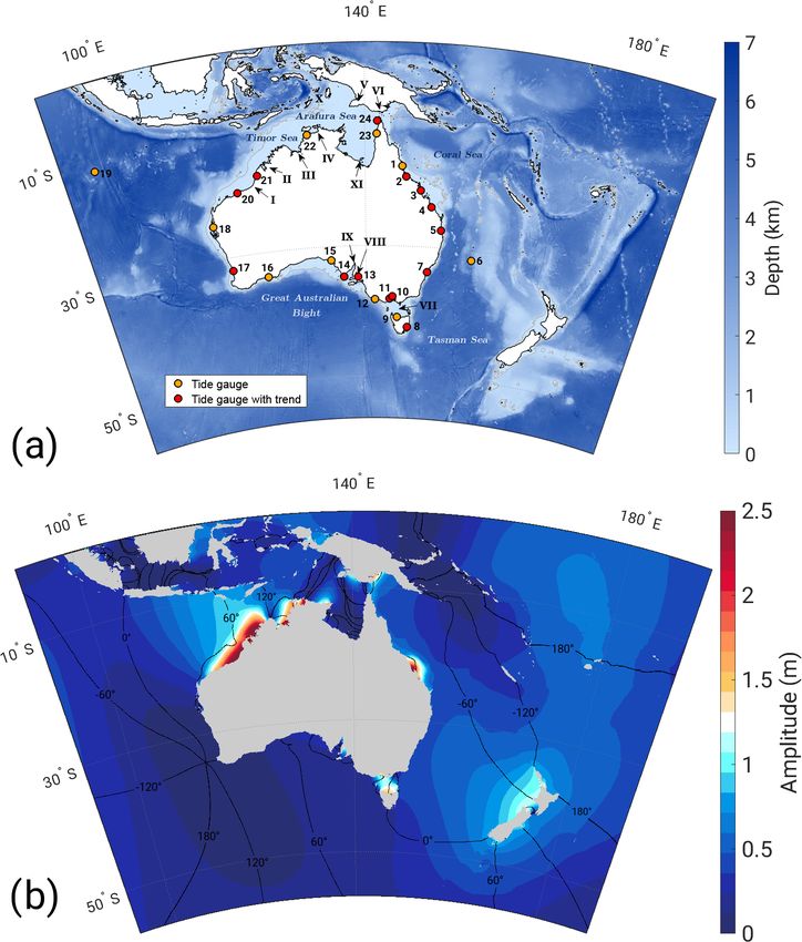
148                                                          A. Harker et al.: The impact of sea-level rise on Australian tides

research, at both regional (Greenberg et al., 2012; Pelling         2     Modelling future tides
et al., 2013; Pelling and Green, 2013; Carless et al., 2016)
and global scales (Müller et al., 2011; Pickering et al., 2017;     2.1    Model configuration and control simulation
Wilmes et al., 2017; Schindelegger et al., 2018).
   Current estimates of the global average change in sea            We use OTIS to simulate the effects of SLR on the tides
level over the last century suggest a rise of between 1.2 and       around Australia. OTIS is a portable, dedicated, numerical
1.7 mm year−1 (Church et al., 2013; Hay et al., 2015; Dan-          shallow water tidal model which has been used extensively
gendorf et al., 2017; IPCC, 2013). However, significant inter-      for both global and regional modelling of past, present, and
annual and decadal-scale fluctuations have occurred during          future ocean tides (e.g. Egbert et al., 2004; Pelling and Green,
this period, for example, over the period 1993–2009, global         2013; Wilmes and Green, 2014; Green et al., 2017). It is
sea-level rise (SLR) has been estimated at 3.2 mm year−1            highly accurate both in the open ocean and in coastal re-
(Church and White, 2011; IPCC, 2013). Studies suggest that          gions (Stammer et al., 2014), and it is computationally ef-
global sea level may rise by up to 1 m by the end of the 21st       ficient. The model solves the linearized shallow-water equa-
century and by up to 3.5 m by the end of the 22nd century           tions (e.g. Hendershott, 1977) given by
(Vellinga et al., 2009; DeConto and Pollard, 2016). However,        ∂U
sea-level change is neither temporally nor spatially uniform,          + f × U = −gH ∇(ζ − ζEQ − ζSAL ) − F                       (1)
                                                                    ∂t
as a multitude of physical processes contribute to regional         ∂ζ
variations (Cazenave and Llovel, 2010; Slangen et al., 2012).          = −∇ · U,                                                  (2)
                                                                    ∂t
Part of this signal is attributed to increasing ocean heat con-
tent causing thermal expansion of the water column, but most        where U is the depth integrated volume transport, which is
of the rise and acceleration in sea level is due to enhanced        calculated as tidal current velocity u multiplied by water
mass input from glaciers and ice sheets (Church et al., 2013).      depth H . f is the Coriolis vector, g denotes the gravitational
The effect of vertical land motion, specifically glacial iso-       constant, ζ stands for the tidal elevation with respect to the
static adjustment (GIA), should also come under considera-          moving seabed, ζSAL denotes the tidal elevation due to ocean
tion; however, around the Australian coastline, the effect is       self-attraction and loading (SAL), and ζEQ is the equilibrium
small (White et al., 2014). Additionally, trends in the am-         tidal elevation. F represents energy losses due to bed fric-
plitude of the M2 constituent around Australia are as much          tion and barotropic–baroclinic conversion at steep topogra-
as 80 % of the magnitude of the trend seen in global MSL            phy. The former is represented by the standard quadratic law:
(Woodworth, 2010); thus, the impact of changing tides upon          FB = Cd u|u|,                                                 (3)
regional variations in sea level should not be underestimated.
   Here, we expand previous tides and SLR investigations to         where Cd = 0.003 is a non-dimensional drag coefficient, and
the shelf seas surrounding Australia, which have received lit-      u is the total velocity vector for all the tidal constituents. The
tle attention so far despite the north-west Australian Shelf        parameterization for internal tide drag, Fw = C|U|, includes
alone being responsible for a large amount of energy dissi-         a conversion coefficient C, which is defined as (Zaron and
pation comparable to that of the Yellow Sea or the Patago-          Egbert, 2006; Green and Huber, 2013)
nian Shelf (Egbert and Ray, 2001). Here, we study the re-
                                                                                  (∇H )2 Nb N
gion’s tidal response to a uniform SLR signal and consider          C(x, y) = γ               .                                   (4)
the impact of coastal defences (inundation of land allowed or                       8π 2 ω
coastal flood defences implemented) on the tidal response.          Here, γ = 50 is a scaling factor, Nb is the buoyancy fre-
Wide areas of this region experience large tides at present,        quency evaluated at the seabed, N is the vertical average of
and areas such as the Gulf of Carpentaria are influenced            the buoyancy frequency, and ω is the frequency of the tidal
by tidal resonances (Webb, 2012). It is therefore expected          constituent under evaluation. Values of both Nb and N fol-
that we will see large differences in the tidal signals with        low from the prescription of horizontally uniform stratifica-
even moderate SLR, as it is known that a (near-)resonant            tion N (z) = N0 exp(−z/1300), where N0 = 5.24 × 10⁻³ s−1
tidal basin is highly sensitive to bathymetric changes (e.g.        has been obtained from a least-squares fit to present-day cli-
Green, 2010). In what follows, we introduce the Oregon State        matological hydrography (Zaron and Egbert, 2006).
University Tidal Inversion Software (OTIS), the dedicated              The model solves Eqs. (1)–(2) using forcing from the
tidal modelling software used, and the simulations performed        astronomical tide-generating potential only (represented by
(Sect. 2.1–2.3). To ground our considerations of future tides       ζEQ in Eq. 1), with the SAL term being derived from TPXO8
on a firm observational basis, we conduct extensive compar-         (Egbert and Erofeeva, 2002, updated version). An initial
isons to tide gauge data in Sect. 2.4. Section 3 presents the       spin-up from rest over 7 days is followed by a further 15 days
results, and the paper concludes in the last section with a dis-    of simulation time, on which harmonic analysis is performed
cussion.                                                            to obtain the tidal elevations and transport. Here, we investi-
                                                                    gate the two dominating semi-diurnal and diurnal tidal con-
                                                                    stituents, M2 and K1 , respectively. The model bathymetry

Ocean Sci., 15, 147–159, 2019                                                                     www.ocean-sci.net/15/147/2019/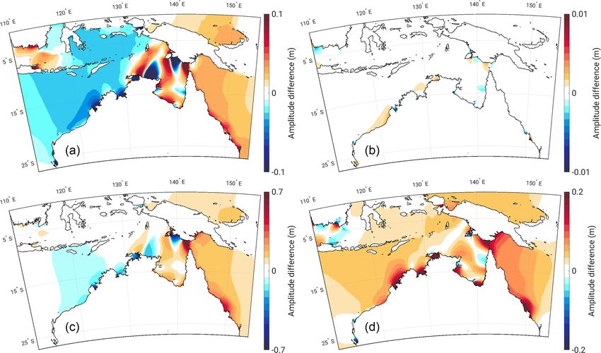
A. Harker et al.: The impact of sea-level rise on Australian tides 149
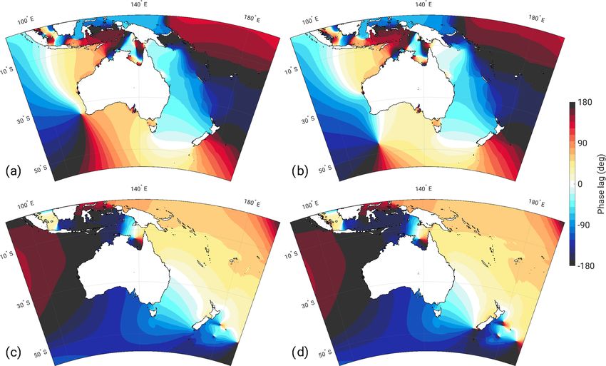
Figure 1. (a) Bathymetry of the model domain and tide gauge sites used in the analysis (coloured dots): see Table 1. Locations at which
M2 trends were estimated are shown in red. Regions mentioned in subsequent sections of the paper are marked on the map: I – Eighty Mile
Beach, II – King Sound, III – Joseph Bonaparte Gulf, IV – Van Diemen Gulf, V – Yos Sudarso Island, VI – Torres Strait, VII – Bass Strait,
VIII – Gulf St. Vincent, IX – Spencer Gulf, X – Arafura Islands, XI – Wellesley Islands. (b) Co-tidal chart of the M2 constituent amplitude
for the control simulation. Black lines represent co-phase lines with 60◦ separation.
comes from the ETOPO1 dataset (Amante and Eakins, 2009, Here, W is the work done by the tide-generating force and
see Fig. 1 for the present domain), which was averaged to P is the energy flux given by
1/20◦ horizontal resolution. For the control run with present-
day water depths, the domain model heights at the open W = gρhU · ∇(ηSAL + ηEQ )i (6)
boundaries were constrained to elevation data from a coarser- P = ghηUi, (7)
resolution global OTIS run, taken from Wilmes et al. (2017).
where the angular brackets mark time averages over a tidal
TPXO8 was used to validate the model (alongside tide gauge
period.
data at 24 locations); see Sect. 2.4.
2.3 Implementing sea-level rise
2.2 Dissipation computations
The model runs are split into two sets. In the first, we al-
The computation of tidal dissipation rates, D, was done fol-
low low-lying grid cells to flood as sea level rises, whereas
lowing Egbert and Ray (2001):
in the second set we introduce vertical walls at the present-
D = W − ∇ · P. (5) day coastline. Following Pelling et al. (2013), we denote
www.ocean-sci.net/15/147/2019/ Ocean Sci., 15, 147–159, 2019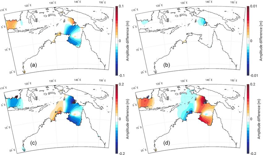
150                                                           A. Harker et al.: The impact of sea-level rise on Australian tides

Table 1. Start and end dates of the analysed tide gauge records,     changes to tidal characteristics across the domain and also
including names and running index for identification in Fig. 1.      correspond to a high but probable level for the end of this
                                                                     century and an extreme case in which large levels of ice sheet
   Station ID    Name                  Time span     Source          collapse has occurred, respectively (e.g. Wilmes et al., 2017).
   1             Mourilyan Harbour     1986–2014     GESLA           The simulations with 12 m of SLR have little physical justi-
   2             Townsville            1980–2014     GESLA           fication, but they allow us to assess how any tidal trends seen
   3             Hay Point             1985–2014     UHSLC           up to 7 m, if they appear, may evolve for even higher levels
   4             Gladstone             1982–2014     UHSLC           of SLR.
   5             Brisbane              1985–2016     GESLA
   6             Lord Howe Island      1992–2014     GESLA           2.4   Model validation
   7             Fort Denison          1965–2017     GESLA
   8             Spring Bay            1986–2017     GESLA           For validation of our numerical experiments, time series of
   9             Burnie                1985–2014     GESLA           hourly sea-level data from 24 stations around Australasia
   10            Williamstown          1976–2014     UHSLC           were obtained from the Global Extreme Sea Level Analysis
   11            Geelong               1976–2014     UHSLC           version 2 (GESLA-2; Woodworth et al., 2017) and the Uni-
   12            Portland              1982–2014     GESLA           versity of Hawaii Sea Level Center (UHSLC; Caldwell et al.,
   13            Port Adelaide         1976–2014     GESLA           2015); see Table 1. With few exceptions, record lengths are
   14            Port Lincoln          1967–2014     UHSLC
                                                                     short, but all time series span at least 28 years to allow for an
   15            Thevenard             1966–2014     GESLA
   16            Esperance             1985–2017     GESLA
                                                                     appropriate representation of the 18.61-year nodal cycle in
   17            Fremantle             1970–2014     GESLA           lunar tidal constituents (Haigh et al., 2011). Upon removal
   18            Carnarvon             1991–2014     GESLA           of years missing more than 25 % of hourly observations,
   19            Cocos Islands         1991–2017     GESLA           a three-tiered least-squares fitting procedure was applied to
   20            Port Hedland          1985–2014     UHSLC           (i) extract mean M2 and K1 tidal constants of amplitude H
   21            Broome                1989–2017     UHSLC           and phase lag G, (ii) deduce linear trends in H and G for
   22            Darwin                1991–2017     GESLA           both constituents over the complete time series at each sta-
   23            Weipa                 1986–2014     GESLA           tion, and (iii) estimate the corresponding long-term trend in
   24            Booby Island          1990–2017     UHSLC           MSL. A total of 10 out of 24 tide gauge stations yielded sta-
                                                                     tistically insignificant M2 amplitude trends at the 95 % con-
                                                                     fidence level and were thus excluded from the model trend
these sets “flood” (FL) and “no flood” (NFL), respectively.          validation below; see Fig. 1 for a graphical illustration.
A range of SLR scenarios corresponding to predicted global              The processing protocol, essentially taken from Schinde-
mean sea-level increases from large-scale ice sheet collapses        legger et al. (2018), is based on a separation of tidal and non-
(Wilmes et al., 2017) are investigated in both sets. This is         tidal residuals from the longer-term MSL component through
done via the implementation of a uniform depth increase              application of a 4-day moving average with Gaussian weight-
across the entire domain of 1, 3, 5, 7, and 12 m. Bound-             ing. The high-frequency filter residuals obtained were then
ary conditions for each of the SLR scenarios are generated           harmonically analysed for 68 tidal constituents using the
from global simulations. The 5, 7, and 12 m SLR NFL runs             Matlab® UTide software package (Codiga, 2011), with anal-
were taken directly from Wilmes et al. (2017) and the re-            ysis windows either set to the entire time series (step i) or
maining global simulations were carried out following the            shifted on an annual basis (step ii). In both cases, we con-
methodology outlined in Wilmes et al. (2017) but with vary-          figured UTide for standard least-squares and a white-noise
ing global sea-level changes and allowing for inundation in          approach in the computation of confidence intervals. Sub-
the FL runs. Additionally, we simulated tidal responses to           sequent regressions of annual M2 tidal constants were per-
future changes in water depth extrapolated from geocentric           formed with a functional model composed of a linear trend,
sea-level trend patterns as observed by satellite altimetry (see     a lag 1-year autocorrelation, AR(1), and sinusoids to account
Carless et al., 2016; Schindelegger et al., 2018). While such        for nodal modulations. Trends in MSL were likewise deter-
projections contain not only the actual long-term trend of sea       mined through regression under AR(1) assumptions, upon a
level but also significant (sub-)decadal variability, little dif-    priori reduction of the influence of the 18.61-year equilib-
ference was found for tidal perturbations with respect to our        rium tide.
uniform SLR scenarios (see the Supplement). It is also un-
known how the magnitude and spatial variation of the trend
pattern may change over the period of time required to equate
a uniform SLR, especially with the larger scenarios consid-
ered here. Hence, in the following, the focus is on the uni-
form SLR scenarios. We choose to show results for the 1
and 7 m SLR simulations because they best exemplify the

Ocean Sci., 15, 147–159, 2019                                                                    www.ocean-sci.net/15/147/2019/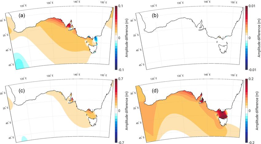
A. Harker et al.: The impact of sea-level rise on Australian tides                                                                    151

Figure 2. The constituent amplitude at each tide gauge position
calculated from GESLA and UHSLC data and the model control
simulation for (a) M2 and (b) K1 . The solid line marks the zero
difference line. The dashed lines mark 1 standard deviation of the   Figure 3. Observed and modelled M2 response coefficients in (a)
difference.                                                          amplitude H and (b) phase lag G per metre of SLR. Model val-
                                                                     ues (red squares) are based on the 1 m FL simulations, while tide
                                                                     gauge estimates at 14 out of 24 locations are shown in black. Error
   A regression of the constituent amplitudes calculated from        bars correspond to 2 standard deviations, propagated from the trend
the OTIS control simulation for the present-day bathymetry           analyses of sea-level and annual tidal estimates of M2 . Stations with
against the M2 and K1 amplitudes from harmonic analysis of           insignificant phase trends (at the 95 % confidence level) are shown
the tide gauge data (Fig. 2) reveals that the model performs         as white markers in panel (b). Numbers at the end of the station
well at all sample sites except at stations Williamstown and         labelling indicate mean observed M2 amplitudes (cm).
Geelong (see Fig. 1 and Table 1). Here, simulated amplitudes
are overestimated by a factor of 5 (M2 ) and 2 (K1 ), respec-
tively. Both of stations lie on the coast of Port Phillip Bay,          Additional comparisons with gridded M2 data were per-
a shallow bay isolated from the Bass Strait by two penin-            formed using the TPXO8 inverse solution, linearly interpo-
sulas. The eastern peninsula is long and narrow, and not re-         lated to the grid of the model domain (see http://volkov.oce.
solved in the model bathymetry due to the spatial averaging          orst.edu/tides, last access: 17 April 2018, for details). The
performed on the source ETOPO1 dataset. As such, the tidal           rms difference between the model and the TPXO8 data is
wave from the Bass Strait penetrates into the bay and builds         7 cm for M2 and 2 cm for K1 . The variance capture (VC)
up in amplitude through reflection at lateral boundaries. Ex-        of the control was also calculated to see how well the over-
cluding Williamstown and Geelong from the comparison, we             all character of the tidal constituents was represented (e.g.
obtain a root mean square (rms) error for the constituent am-        Pelling and Green, 2013):
plitudes of 17 cm for M2 and 2 cm for K1 , while correlation                    "                #
                                                                                         RMSD 2

coefficients are at 0.97 and 0.99, respectively. Estimates of
                                                                     VC = 100 1 −                   ,                           (8)
the median absolute difference between model and test sta-                                  S
tions can be used to quantify possible biases in a robust way
(Stammer et al., 2014); corresponding values are 8 cm for            where RMSD is the rms difference between the control simu-
M2 and 1 cm for K1 irrespective of whether stations in Port          lation and TPXO8, and S denotes the rms standard deviation
Phillip Bay are included or not. Median phase differences            of the TPXO8 amplitudes. The VC is above 96 % for M2 and
with respect to the tide gauge estimates are 21◦ for M2 and          97 % for K1 .
3◦ for K1 . These statistics give confidence in the model’s ac-         For validation of the simulated M2 changes under SLR,
curacy and in the assertion that areas where the disagreement        we followed Schindelegger et al. (2018) and condensed mea-
between model and tide gauge data is largest are where the           sured M2 trends (∂H , ∂G) and MSL rates (∂s) to response
resolution of the model has not resolved fine-structure coastal      coefficients in amplitude (rH = ∂H /∂s) and phase (rG =
features.                                                            ∂G/∂s). Simulated amplitude and phase changes from the

www.ocean-sci.net/15/147/2019/                                                                        Ocean Sci., 15, 147–159, 2019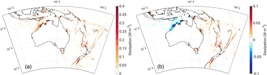
152                                                              A. Harker et al.: The impact of sea-level rise on Australian tides

Figure 4. The constituent phase lags with respect to the Greenwich meridian (◦ ) for the control (a, c) and 7 m SLR (b, d) simulations for M2
(a, b) and K1 (c, d).

1 m FL run at the location of 14 tide gauges were interpo-               transport induced by thermocline deepening (Müller, 2012),
lated from nearest-neighbour cells and also converted to ra-             need to be thoroughly addressed to complete the picture of
tios of rH and rG . Graphical comparisons in Fig. 3 indicate             secular changes in the surface tide. Furthermore, uncertainty
that the model captures the sign of the observed M2 ampli-               in the bathymetric data due to sparsity of sounding observa-
tude response in 10 out of 14 cases and reproduces large frac-           tions may induce additional errors. Despite these limitations,
tions of the in situ variability at approximately half of the            our 1 m FL simulation captures good portions of the patterns
analysed stations (e.g. Booby Island, Brisbane, Geelong, Port            of M2 amplitude changes seen in tide gauge records around
Hedland, Broome). A similar figure for K1 can be found in                Australasia. Moreover, on timescales of centuries, water col-
the supporting information. Model-to-data disparities on the             umn depth changes due to SLR will outweigh tidal pertur-
northeastern seaboard (Hay Point, Gladstone) are markedly                bations from other physical mechanisms. Hence, we con-
reduced in comparison to Schindelegger et al. (2018, their               clude that our simulations lend themselves well for analysis
Fig. 7) due to the higher horizontal resolution of our setup             of probable future tidal changes over a wider area.
in a region of ragged coastline features. Neither the increase
of M2 amplitudes at Townsville nor the pronounced reduc-
tion of the tide at Fort Denison (Sydney Harbour) can be ex-             3   Results
plained by SLR perturbations in the tidal model; both signals
may be the effect of periodic dredging to maintain accept-               The control run exemplifies the typical tidal environment of
able water depths for port operations; see Devlin et al. (2014)          the model domain (Figs. 1b and 4a). M2 has large amplitudes
for a similar analysis. The decrease of the small M2 tide at             along the north-west coast of Australia and within Joseph
Spring Bay, Tasmania (20 cm m−1 of SLR), remains puzzling                Bonaparte Gulf and Van Diemen Gulf. To the south-west of
though, given that the gauge is open to the sea and unaffected           Australia lies a clockwise-rotating amphidrome, responsible
by harbour activities or variable river discharge rates. Mech-           for the westward propagation of the tidal wave across the
anisms other than SLR, such as modulation of the internal                north Australian Shelf. The interaction of this wave with the
tide due to stratification changes along its path of propa-              confined topography of the Arafura Sea leads to a complex
gation (Colosi and Munk, 2006) or variations in barotropic               tidal pattern with a notable amphidrome north of the Gulf

Ocean Sci., 15, 147–159, 2019                                                                          www.ocean-sci.net/15/147/2019/
A. Harker et al.: The impact of sea-level rise on Australian tides                                                                       153

Figure 5. The difference in M2 amplitude (m) between the FL and control simulation (i.e. FL–control) for 1 m SLR (a) and 7 m SLR (c)
alongside the difference between the NFL and FL simulations (i.e. NFL–FL) for 1 m SLR (b) and 7 m SLR (d). The scale applied to panels (a)
and (c) is relative to the applied SLR scenario. Regions that appear blue in panels (b) and (d) are where the FL amplitude is greater than the
NFL amplitude; as such, coastal areas which have been flooded will appear blue.

of Carpentaria. The tide rotates anti-clockwise around New               3.1    Effect of SLR on the M2 tide
Zealand towards the east coast of Australia, where large am-
plitudes can be seen between Hay Point and Gladstone. K1 is              SLR brings some fairly significant changes to the M2 tidal
dominated by a single amphidrome located within the Gulf                 systems around Australia. Many of the regions which stand
of Carpentaria, with raised amplitudes to the north and south            out as having high M2 amplitude at present (see Fig. 1b)
of this point (see the Supplement).                                      suffer a marked reduction in amplitude with increasing SLR
   In general, for both constituents, the amplitude changes              (Fig. 5a and c). To the north-west of Australia, amplitudes de-
are not linear with respect to the imposed level of SLR (see             crease in regions centred around King Sound, around Joseph
Idier et al., 2017; Pickering et al., 2017, where tidal ampli-           Bonaparte Gulf, within Van Diemen Gulf, and across the
tudes across the European Shelf changed non-proportionally               Timor Sea. The reduction in amplitude to the north-east of
with SLR greater than 2 m). Relative changes are larger for              Van Diemen Gulf comes alongside the formation of a new
lower SLR scenarios (e.g. 1 m) than for the higher SLR sce-              amphidrome; the phase lines that run north-south in the Ara-
narios (e.g. 7 m). No significant differences between the FL             fura Sea (Fig. 1b) move closer together before coalescing to
and NFL scenarios for 1 m SLR can be seen, likely due to the             form an amphidromic point. A further amphidromic point
fact that allowing land to flood at a 1 m SLR scenario only in-          emerges in the south-east of the Gulf of Carpentaria, around
creased the wetted area by 12 grid cells (on our 1166 × 2000             the Wellesley Islands, when a virtual amphidromic point (an
computational grid), while at 7 m SLR 3320 new ocean grid                amphidrome over land) moves north to become real (an am-
cells were generated. Accordingly, for larger sea-level in-              phidrome over the ocean). Both these points form some time
creases, the differences between the Fl and NFL scenarios                between 3 and 5 m SLR (not shown). The amphidrome that
become more pronounced due to the increased number of                    sits north of the Gulf of Carpentaria (Fig. 4a) moves north-
flooded cells. A detailed analysis of the impact of SLR on               wards with SLR in both the FL and NFL scenarios, eventu-
M2 , and more peripherally K1 , is given below; the most com-            ally becoming virtual at the higher SLR scenarios by moving
mon locations discussed are shown in Fig. 1a.                            over Yos Sudarso Island. This movement is therefore asso-
                                                                         ciated with the change in the propagation properties of the

www.ocean-sci.net/15/147/2019/                                                                            Ocean Sci., 15, 147–159, 2019
154 A. Harker et al.: The impact of sea-level rise on Australian tides Figure 6. Same as Fig. 5 but showing the south coast of Australia. incoming tidal wave, rather than the inundation of Yos Su- the imposed level of SLR (see Fig. 6c for the 7 m case). To darso Island which occurs at 5 m SLR and above. the east, in Gulf St. Vincent, there is a similar, if stronger, The Torres Strait features a sharp divide between a large standing-wave-like pattern (Fig. 1b). Here, the elevated am- positive and small or weakly negative amplitude difference plitudes proximity to the coast increase in line with SLR on its west and east sides, respectively. The strait is shallow (Fig. 6c). Moving further west along the south coast of Aus- and dotted with islands, restricting the flow of the tides. Ab- tralia, the amphidromic point off the south-west coast moves solute amplitudes on the east side are initially elevated com- southwards with increasing SLR (Fig. 4a and b), with a faster pared to the west (Fig. 1b) but this difference is mitigated progression in the NFL than in the FL runs. Note that, al- with increasing SLR, as the larger volume of the channel al- most universally across the domain, the amplitudes seen in lows for enhanced tidal transport across the strait (Fig. 5a the NFL runs are higher than those in the FL runs (Figs. 5d and c). and 6d). It is clear that allowing flooding to occur suppresses In the remaining part of the domain, the M2 amplitudes the magnitude of any SLR effect upon tidal amplitude. around the coast of New Zealand and along the east coast Additionally, we have repeated our control and future sim- of Australia, particularly between Hay Point and Gladstone ulations using boundary conditions taken from TPXO8, i.e. (Fig. 1a, points 3 and 4), both increase with SLR. In the Bass using present-day boundary conditions, instead of those from Strait, shown in Fig. 6, the amplitude also increases along global SLR simulations. In these runs, the magnitude and with SLR; however, there is a slight drop in amplitude at spatial distribution of the amplitude changes are vastly dif- 1 m SLR at the eastern entrance of the strait and within Port ferent from the results presented above. Figure 7 demon- Phillip Bay (the location of the Geelong and Williamstown strates, and allows for a comparison of, the pattern of am- tide gauges). These decreases quickly disappear at higher plitude changes seen for M2 north of Australia in these runs. SLR. Along the south coast of Australia, the amplitudes also Especially striking is the difference in magnitude of tidal am- increase with SLR, but the simulated perturbations there are plitude increases along the east coast of Australia. Apply- generally smaller in magnitude than in the north (see also ing present-day boundary conditions leads to a very strong Schindelegger et al., 2018). Increased tidal amplitudes at the underestimation of the amplitude changes in this area (the head and mouth of Spencer Gulf (Fig. 6a) are associated with differences exceed 40 cm in some locations). Similarly pro- a slight weakening of a standing-wave-like pattern where M2 nounced is the difference on the north-west coast where the amplitudes increase from the sea towards inland (Fig. 1b). run with present-day boundary conditions overestimates the However, this feature does not evolve proportionally with amplitude decreases. In large parts of the Arafura Sea, the Ocean Sci., 15, 147–159, 2019 www.ocean-sci.net/15/147/2019/
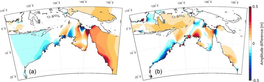
A. Harker et al.: The impact of sea-level rise on Australian tides                                                                     155

Figure 7. The difference in M2 amplitude (m) between the FL and control simulation (i.e. FL–control) for 7 m SLR using boundary conditions
generated from a global 7 m SLR scenario (a) and using boundary conditions generated from TPXO8 (b).

Figure 8. The dissipation (W m−2 ) associated with the M2 constituent across the entire model domain (a) and the difference in dissipation
between the 7 m FL simulation and the control run (i.e. FL–control, b).

tidal amplitude responses are of opposite sign in response to
the different boundary conditions. This is a key result and it
highlights the importance of applying correct boundary con-
ditions for regional simulations which take into account the
far-field change occurring outside the model domain.
   Figure 8a displays the dissipation associated with the M2
tidal constituent for the control simulation. It is evident that
a majority of the energy is lost at the coast and on the
shelf, especially around sharp and shallow bathymetric fea-
tures. There is a remarkable reduction in dissipation along
the north-west coast of Australia with SLR, matching areas
with a marked decrease in tidal amplitude (Fig. 8b). There
are small pockets of dissipation increases in proximity to the
coast in the north-west, associated with areas of enhanced
flooding. Much of the dissipation increases within the do-
main come from the undersea ridges and trenches to the north
and south of New Zealand, as well as the east side of the Tor-         Figure 9. The dissipation totals (GW) across the model domain
res Strait, the area between Hay Point and Gladstone on the            above and below (inset) the depth of the 200 m isobath of the control
east coast of Australia (at the southern extent of the Great           bathymetry.
Barrier Reef), and both ends of the Bass Strait. All of these

www.ocean-sci.net/15/147/2019/                                                                          Ocean Sci., 15, 147–159, 2019
156                                                        A. Harker et al.: The impact of sea-level rise on Australian tides

Figure 10. Same as Fig. 5 but for the K1 constituent.

areas are associated with an increase in M2 amplitude with        phase plots in Fig. 4c and d, and it is evident that K1 suf-
SLR.                                                              fers a decrease in amplitude around the Gulf of Carpentaria
   The impact upon the total dissipation across the domain        with SLR. Comparing Fig. 10c and d, a majority of the am-
by allowing flooding is illustrated in Fig. 9. In both the NFL    plitude difference occurring in the FL scenario is negated
and FL runs, dissipation increases with SLR; the dissipation      when impermeable coastlines are implemented. The dissipa-
generated by areas with increased amplitudes outweighs the        tion for which K1 is responsible in the domain is approx-
loss of dissipation in areas of decreased amplitude. With am-     imately 7 times smaller than that of M2 and therefore not
plitudes in the NFL runs being much higher than in the FL         discussed further.
runs, the corresponding dissipation is higher, and the gap in
dissipation between the NFL and FL simulations widens with        3.3   Synthesis
increasing SLR. At 12 m SLR, the NFL dissipation begins to
plateau, whilst the FL dissipation continues to rise. Overall,    One of the most striking characteristics of the response of
dissipation on the shelf (nominally above the 200 m isobath,      the semi-diurnal constituents to SLR is the drop in amplitude
accounting for approximately 7 % of the water-covered area        along the north-west coast of Australia, an area where a large
of the domain) amounts to about half of the energy dissipated     amount of dissipation occurs in the control. We associate this
in deeper water.                                                  feature with the altered propagation properties of the incom-
                                                                  ing tidal wave, as the imposed sea-level change in our simu-
3.2   Effect of SLR on the K1 tide                                lations represents a significant fraction of the average water
                                                                  depth across the shelf; for instance, the 7 m SLR scenario in-
The changes to K1 are relatively small in comparison to           creases the depth of the Gulf of Carpentaria by ∼ 10 %. As
the changes seen for the semi-diurnal constituent. The main       the tidal system goes from hosting a single wave propagat-
point of interest is the amphidromic system in the Gulf of        ing across the Arafura Sea to something more complex with
Carpentaria. Figure 10 shows an initial negative amplitude        multiple amphidromes within the basin, the semi-diurnal res-
response in the north and south of the Gulf, while there are      onant response on the shelf is interrupted. This dynamical
slight increases in amplitude north of Yos Sudarso Island and     change may explain the drop in amplitudes to the north-west
in the Java Sea. The position of the amphidromic system is        of Australia.
relatively stable with SLR, as evident from the constituent

Ocean Sci., 15, 147–159, 2019                                                                www.ocean-sci.net/15/147/2019/
A. Harker et al.: The impact of sea-level rise on Australian tides 157
4 Discussion cant impact on the response of the tide by locally increasing
dissipation and should be considered essential for future tidal
It has been shown here, using a validated tidal model, that modelling with SLR.
the tidal characteristics around Australia are sensitive to wa-
ter column depth changes due to SLR. We show significant
changes in tidal amplitudes due to the SLR, with the largest Data availability. The sea-level data came from UHSLC
change in amplitude being 15 % of the SLR signal south of (https://doi.org/10.7289/V5V40S7W, Caldwell et al., 2015) and
Papua New Guinea and north-east of Van Diemen Gulf. The GESLA-2 (https://doi.org/10.5285/3b602f74-8374-1e90-e053-
model can reproduce considerable fractions of the tidal am- 6c86abc08d39, Woodworth et al., 2017). Model results are
available from the authors upon request.
plitude change signals seen in the tide gauge record. This is
a strong indication that the observed changes in tides are, at
least in part, driven by sea-level changes, and adds further
Supplement. The supplement related to this article is available
motivation for our investigation. online at: https://doi.org/10.5194/os-15-147-2019-supplement.
Somewhat surprisingly, the responses of the tides to SLR
are very different in both their sign and spatial patterns de-
pending on how the open boundary conditions are imple- Author contributions. The experiments were originally carried out
mented. Furthermore, in the simulations with TPXO8 data on by AH as a student under the supervision of JAMG. JAMG per-
the open boundary, the amplitude changes along the north- formed further regional model runs utilising data from SBW’s
east coast, home to several population centres, are strongly global simulations. MS performed the model validation. AH pre-
underestimated. The take-home message here is that, oppo- pared the manuscript with contributions from all co-authors.
site to what has often been assumed (e.g. Pelling and Green,
2013), simulations of the effect of SLR on tides for cer-
tain regions should not use present-day boundary conditions, Competing interests. The authors declare that they have no conflict
even if the open boundary is in the far field. There are also of interest.
pronounced differences between the FL and NFL simula-
tions. Consequently, to make accurate predictions of the fu-
ture tides, local coastal defence strategies need to be known, Special issue statement. This article is part of the special
because allowing land to flood could mitigate increases in the issue “Developments in the science and history of tides
(OS/ACP/HGSS/NPG/SE inter-journal SI)”. It is not associ-
tidal range induced by the rising sea level. If this information
ated with a conference.
is not obtainable, both scenarios need to be investigated.
However, this introduces another problem: most of Aus-
tralia’s largest cities lie on or near the coast, and many of
Acknowledgements. Financial support for this study was made
them are close to the areas which may experience the largest available by the UK Natural Environmental Research Council
tidal changes with SLR. It thus opens for an interesting in- (grant NE/I030224/1, awarded to J. A. Mattias Green) and the Aus-
vestigation to see if unpopulated areas of the coastline could trian Science Fund (FWF, through project P30097-N29 awarded to
be flooded to mitigate the rising sea level in a hybrid NFL– Michael Schindelegger). All numerical simulations were performed
FL scenario. Adopting a more dynamical perspective, nu- using HPC Wales’ supercomputer facilities.
merical tests employing wave forcing of different periods
are proposed to distinguish if the tidal response of certain Edited by: Philip Woodworth
areas within the domain is largely due to resonance or fric- Reviewed by: two anonymous referees
tional effects (Idier et al., 2017). Additionally, an investiga-
tion into the coupling of tidal changes for expected magni-
tudes of SLR and storm surges (Muis et al., 2016) within the
domain could provide further insight and guidance to the fu- References
ture planning of coastal defences around Australia.
In conclusion, the series of simulations presented here ABS: Australia (AUST) 2011/2016 Census QuickStats,
have shown that the tidal amplitudes along the northern coast Australian Bureau of Statistics (ABS), available at:
of Australia and around the Sahul Shelf region are partic- http://quickstats.censusdata.abs.gov.au/census_services/
getproduct/census/2016/quickstat/036?opendocument (last
ularly sensitive to SLR. Coastal population centres such as
access: 9 November 2018), 2016.
Adelaide and Mackay are predicted to have to deal with
Allen, G. P., Salomon, J. C., Bassoullet, P., Penhoat, Y. D., and
the consequences of increased tidal amplitudes with increas- de Grandpré, C.: Effects of tides on mixing and suspended sedi-
ing SLR. SLR appears to be moving the semi-diurnal con- ment transport in macrotidal estuaries, Sediment. Geol., 26, 69–
stituents away from resonance on the shelf and only have a 90, https://doi.org/10.1016/0037-0738(80)90006-8, 1980.
small impact on the diurnal constituents in the Gulf of Car- Amante, C. and Eakins, B. W.: ETOPO1 1 arcmin Global Relief
pentaria. The implementation of flooding can have a signifi- Model: Procedures, Data Sources and Analysis, NOAA Tech-
www.ocean-sci.net/15/147/2019/ Ocean Sci., 15, 147–159, 2019158 A. Harker et al.: The impact of sea-level rise on Australian tides nical Memorandum NESDIS NGDC-24, National Geophysical Greenberg, D. A., Blanchard, W., Smith, B., and Bar- Data Center, NOAA, https://doi.org/10.7289/V5C8276M, 2009. row, E.: Climate change, mean sea level and high tides Caldwell, P. C., Merrifield, M. A., and Thompson, P. R.: Sea in the Bay of Fundy, Atmos. Ocean, 50, 261–276, level measured by tide gauges from global oceans – the Joint https://doi.org/10.1080/07055900.2012.668670, 2012. Archive for Sea Level holdings (NCEI Accession 0019568), Haigh, I. D., Eliot, M., and Pattiaratchi, C.: Global influences of NOAA National Centers for Environmental Information, Version the 18.61 year nodal cycle and 8.85 year cycle of lunar perigee 5.5, Dataset, https://doi.org/10.7289/V5V40S7W, 2015. on high tidal levels, J. Geophys. Res.-Oceans, 116, C06025, Carless, S., Green, J., Pelling, H., and Wilmes, S.-B.: Ef- https://doi.org/10.1029/2010JC006645, 2011. fects of future sea-level rise on tidal processes on Hay, C. C., Morrow, E., Kopp, R. E., and Mitrovica, J. X.: Prob- the Patagonian Shelf, J. Marine Syst., 163, 113–124, abilistic reanalysis of twentieth-century sea-level rise, Nature, https://doi.org/10.1016/j.jmarsys.2016.07.007, 2016. 517, 481–484, https://doi.org/10.1038/nature14093, 2015. Cazenave, A. and Llovel, W.: Contemporary Sea Level Rise, Ann. Hendershott, M. C.: Numerical models of ocean tides, in: The Sea, Rev. Mar. Sci., 2, 145–173, https://doi.org/10.1146/annurev- vol. 6, 47–89, Wiley Interscience Publication, 1977. marine-120308-081105, 2010. Idier, D., Paris, F., Le Cozannet, G., Boulahya, F., and Church, J. A. and White, N. J.: Sea-Level Rise from the Late Dumas, F.: Sea-level rise impacts on the tides of 19th to the Early 21st Century, Surv. Geophys., 32, 585–602, the European Shelf, Cont. Shelf Res., 137, 56–71, https://doi.org/10.1007/s10712-011-9119-1, 2011. https://doi.org/10.1016/j.csr.2017.01.007, 2017. Church, J. A., Monselesan, D., Gregory, J. M., and Marzeion, IPCC: Climate Change 2013: The Physical Science Basis, Con- B.: Evaluating the ability of process based models to tribution of Working Group I to the Fifth Assessment Re- project sea-level change, Environ. Res. Lett., 8, 014051, port of the Intergovernmental Panel on Climate Change, Cam- https://doi.org/10.1088/1748-9326/8/1/014051, 2013. bridge University Press, Cambridge, UK, New York, NY, USA, Codiga, D. L.: Unified tidal analysis and prediction using the UTide https://doi.org/10.1017/CBO9781107415324, 2013. Matlab functions, Graduate School of Oceanography, University McInnes, K. L., Church, J., Monselesan, D., Hunter, J. R., O’Grady, of Rhode Island Narragansett, RI, 2011. J. G., Haigh, I. D., and Zhang, X.: Information for Australian im- Colosi, J. A. and Munk, W.: Tales of the venerable Hon- pact and adaptation planning in response to sea-level rise, Aust. olulu tide gauge, J. Phys. Oceanogr., 36, 967–996, Meteorol. Ocean, 65, 127–149, 2015. https://doi.org/10.1175/JPO2876.1, 2006. Muis, S., Verlaan, M., Winsemius, H. C., Aerts, J. C. Dangendorf, S., Marcos, M., Wöppelmann, G., Conrad, C. P., Fred- J. H., and Ward, P. J.: A global reanalysis of storm erikse, T., and Riva, R.: Reassessment of 20th century global surges and extreme sea levels, Nat. Commun., 7, 11969, mean sea level rise, P. Natl. Acad. Sci. USA, 114, 5946–5951, https://doi.org/10.1038/ncomms11969, 2016. https://doi.org/10.1073/pnas.1616007114, 2017. Müller, M.: The influence of changing stratification conditions DeConto, R. M. and Pollard, D.: Contribution of Antarctica on barotropic tidal transport and its implications for seasonal to past and future sea-level rise, Nature, 531, 591–597, and secular changes of tides, Cont. Shelf Res., 47, 107–118, https://doi.org/10.1038/nature17145, 2016. https://doi.org/10.1016/j.csr.2012.07.003, 2012. Devlin, A. T., Jay, D. A., Talke, S. A., and Zaron, E.: Can Müller, M., Arbic, B. K., and Mitrovica, J. X.: Secular trends in tidal perturbations associated with sea level variations in ocean tides: Observations and model results, J. Geophys. Res.- the western Pacific Ocean be used to understand future ef- Oceans, 116, C05013, https://doi.org/10.1029/2010JC006387, fects of tidal evolution?, Ocean Dynam., 64, 1093–1120, 2011. https://doi.org/10.1007/s10236-014-0741-6, 2014. Pelling, H. E. and Green, J. A. M.: Sea level rise and tidal power Egbert, G. D. and Erofeeva, S. Y.: Efficient inverse modeling of plants in the Gulf of Maine, J. Geophys. Res.-Oceans, 118, 2863– barotropic ocean tides, J. Atmos. Ocean. Tech., 19, 183–204, 2873, https://doi.org/10.1002/jgrc.20221, 2013. https://doi.org/10.1175/JPO2876.1, 2002. Pelling, H. E., Green, J. A. M., and Ward, S. L.: Modelling tides and Egbert, G. D. and Ray, R. D.: Estimates of M2 tidal sea-level rise: To flood or not to flood, Ocean Model., 63, 21–29, energy dissipation from Topex/Poseidon altimeter https://doi.org/10.1016/j.ocemod.2012.12.004, 2013. data, J. Geophys. Res.-Oceans, 106, 22475–22502, Pickering, M., Horsburgh, K. J., Blundell, J. R., Hirschi, J. J.-M., https://doi.org/10.1029/2000JC000699, 2001. Nicholls, R. J., Verlaan, M., and Wells, N. C.: The impact of Egbert, G. D., Bills, B. G., and Ray, R. D.: Numerical model- future sea-level rise on the global tides, Cont. Shelf Res., 142, ing of the global semidiurnal tide in the present day and in the 50–68, https://doi.org/10.1016/j.csr.2017.02.004, 2017. last glacial maximum, J. Geophys. Res.-Oceans, 109, C03003, Pugh, D. and Woodworth, P.: Sea-Level Science: Understanding https://doi.org/10.1029/2003JC001973, 2004. tides, surges, tsunamis and mean sea-level changes, Cambridge Green, J., Huber, M., Waltham, D., Buzan, J., and Wells, M.: University Press, Cambridge, UK, 2014. Explicitly modeled deep-time tidal dissipation and its impli- Schindelegger, M., Green, J. A. M., Wilmes, S.-B., and Haigh, cation for Lunar history, Earth Planet. Sc. Lett., 461, 46–53, I. D.: Can we model the effect of observed sea level https://doi.org/10.1016/j.epsl.2016.12.038, 2017. rise on tides?, J. Geophys. Res.-Oceans, 123, 4593–4609, Green, J. A. M.: Ocean tides and resonance, Ocean Dynam., 60, https://doi.org/10.1029/2018JC013959, 2018. 1243–1253, https://doi.org/10.1007/s10236-010-0331-1, 2010. Slangen, A. B. A., Katsman, C. A., van de Wal, R. S. W., Green, J. A. M. and Huber, M.: Tidal dissipation in the early Eocene Vermeersen, L. L. A., and Riva, R. E. M.: Towards re- and implications for ocean mixing, Geophys. Res. Lett., 40, gional projections of twenty-first century sea-level change based 2707–2713, https://doi.org/10.1002/grl.50510, 2013. Ocean Sci., 15, 147–159, 2019 www.ocean-sci.net/15/147/2019/
A. Harker et al.: The impact of sea-level rise on Australian tides                                                                       159

   on IPCC SRES scenarios, Climate Dynam., 38, 1191–1209,                White, N. J., Haigh, I. D., Church, J. A., Koen, T., Wat-
   https://doi.org/10.1007/s00382-011-1057-6, 2012.                        son, C. S., Pritchard, T. R., Watson, P. J., Burgette,
Stammer, D., Ray, R. D., Andersen, O. B., Arbic, B. K., Bosch,             R. J., McInnes, K. L., You, Z.-J., Zhang, X., and Tre-
   W., Carrère, L., Cheng, Y., Chinn, D. S., Dushaw, B. D., Egbert,        goning, P.: Australian sea levels–Trends, regional variabil-
   G. D., Erofeeva, S. Y., Fok, H. S., Green, J. A. M., Griffiths, S.,     ity and influencing factors, Earth-Sci. Rev., 136, 155–174,
   King, M. A., Lapin, V., Lemoine, F. G., Luthcke, S. B., Lyard,          https://doi.org/10.1016/j.earscirev.2014.05.011, 2014.
   F., Morison, J., Müller, M., Padman, L., Richman, J. G., Shriver,     Wilmes, S.-B. and Green, J. A. M.: The evolution of tides and tidally
   J. F., Shum, C. K., Taguchi, E., and Yi, Y.: Accuracy assessment        driven mixing over 21,000 years, J. Geophys. Res.-Oceans, 119,
   of global barotropic ocean tide models, Rev. Geophys., 52, 243–         4083–4100, https://doi.org/10.1002/2013JC009605, 2014.
   282, https://doi.org/10.1002/2014RG000450, 2014.                      Wilmes, S.-B., Green, J. A. M., Gomez, N., Rippeth, T. P.,
Stumpf, R. P. and Haines, J. W.: Variations in Tidal Level in the Gulf     and Lau, H.: Global tidal impacts of large-scale ice sheet
   of Mexico and Implications for Tidal Wetlands, Estuar. Coast            collapses, J. Geophys. Res.-Oceans, 122, 8354–8370,
   Shelf S., 46, 165–173, https://doi.org/10.1006/ecss.1997.0276,          https://doi.org/10.1002/2017JC013109, 2017.
   1998.                                                                 Woodworth, P. L.: A survey of recent changes in the main com-
Vellinga, P., Katsman, C., Sterl, A., Beersma, J. J., Hazeleger, W.,       ponents of the ocean tide, Cont. Shelf Res., 30, 1680–1691,
   Church, J., Kopp, R., Kroon, D., Oppenheimer, M., Plag, H. P.,          https://doi.org/10.1016/j.csr.2010.07.002, 2010.
   Rahmstorf, S., Lowe, J., Ridley, J., von Storch, H., Vaughan, D.,     Woodworth, P. L., Hunter, J. R., Marcos, M., Caldwell, P.,
   van der Wal, R., Weisse, R., Kwadijk, J., Lammersen, R., and            Menéndez, M., and Haigh, I.: Towards a global higher-
   Marinova, N. A.: Exploring high-end climate change scenarios            frequency sea level dataset, Geosci. Data J., 3, 50–59,
   for flood protection of the Netherlands, Tech. rep., Royal Nether-      https://doi.org/10.1002/gdj3.42, 2017.
   lands Meteorological Institute, 2009.                                 Zaron, E. D. and Egbert, G. D.: Estimating open-ocean barotropic
Watson, P. J.: Is There Evidence Yet of Acceleration in Mean Sea           tidal dissipation: the Hawaiian ridge, J. Phys. Oceanogr., 36,
   Level Rise around Mainland Australia?, J. Coastal Res., 27, 369–        1019–1035, https://doi.org/10.1175/JPO2878.1, 2006.
   377, 2011.                                                            Zhang, X., Church, J. A., Monselesan, D., and McInnes,
Webb, D. J.: On the shelf resonances of the Gulf of Car-                   K. L.: Sea level projections for the Australian region
   pentaria and the Arafura Sea, Ocean Sci., 8, 733–750,                   in the 21st century, Geophys. Res. Lett., 44, 8481–8491,
   https://doi.org/10.5194/os-8-733-2012, 2012.                            https://doi.org/10.1002/2017GL074176, 2017.

www.ocean-sci.net/15/147/2019/                                                                            Ocean Sci., 15, 147–159, 2019
You can also read