Physical drivers of the nitrate seasonal variability in the Atlantic cold tongue
←
→
Page content transcription
If your browser does not render page correctly, please read the page content below
Biogeosciences, 17, 529–545, 2020
https://doi.org/10.5194/bg-17-529-2020
© Author(s) 2020. This work is distributed under
the Creative Commons Attribution 4.0 License.

Physical drivers of the nitrate seasonal variability in the
Atlantic cold tongue
Marie-Hélène Radenac1 , Julien Jouanno1 , Christine Carine Tchamabi1,† , Mesmin Awo1,2,3 , Bernard Bourlès4 ,
Sabine Arnault5 , and Olivier Aumont5
1 LEGOS,   IRD-Université Paul Sabatier-Observatoire Midi-Pyrénées, Toulouse, 31400, France
2 Nansen-Tutu  Centre for Marine Environmental Research, Department of Oceanography,
University of Cape Town, Cape Town, South Africa
3 LHMC, IRHOB, IRD, Cotonou, Benin
4 IRD, US191 “Instrumentation, Moyens Analytiques, Observatoires en Géophysique et Océanographie” (IMAGO),

Technopole Pointe du Diable, Plouzané, France
5 LOCEAN, CNRS, IRD, Sorbonne Universités, MNHN, Paris, 75005, France
† deceased

Correspondence: Marie-Hélène Radenac (marie-helene.radenac@legos.obs-mip.fr)

Received: 26 August 2019 – Discussion started: 18 September 2019
Revised: 18 December 2019 – Accepted: 24 December 2019 – Published: 31 January 2020

Abstract. Ocean color observations show semiannual varia-          1   Introduction
tions in chlorophyll in the Atlantic cold tongue with a main
bloom in boreal summer and a secondary bloom in Decem-
ber. In this study, ocean color and in situ measurements and       Variations in the equatorial upwelling in the Atlantic Ocean
a coupled physical–biogeochemical model are used to inves-         are essentially seasonal. The so-called cold tongue spreads
tigate the processes that drive this variability. Results show     east of about 20◦ W to the African coast and is centered
that the main phytoplankton bloom in July–August is driven         slightly south of the Equator (Carton and Zhou, 1997; Ca-
by a strong vertical supply of nitrate in May–July, and the        niaux et al., 2011). The maximum cooling is reached in
secondary bloom in December is driven by a shorter and             July–August and a secondary cooling occurs in November–
moderate supply in November. The upper ocean nitrate bal-          December (Okumura and Xie, 2006). The cold tongue is
ance is analyzed and shows that vertical advection controls        a region of enhanced biological production mainly driven
the nitrate input in the equatorial euphotic layer and that ver-   by nitrate supply (Voituriez and Herbland, 1977; Loukos
tical diffusion and meridional advection are key in extending      and Mémery, 1999). There, the availability of nutrients af-
and shaping the bloom off Equator. Below the mixed layer,          fects the equatorial ecosystem from primary production to
observations and modeling show that the Equatorial Under-          high trophic levels and CO2 fluxes (Hisard, 1973; Voituriez
current brings low-nitrate water (relative to off-equatorial       and Herbland, 1977; Oudot and Morin, 1987; Loukos and
surrounding waters) but still rich enough to enhance the cold      Mémery, 1999; Ménard et al., 2000; Christian and Mur-
tongue productivity. Our results also give insights into the       tugudde, 2003; Lefèvre, 2009). Early in situ measurements
influence of intraseasonal processes in these exchanges. The       in the equatorial Atlantic (Hisard, 1973; Voituriez and Herb-
submonthly meridional advection significantly contributes to       land, 1977) evidenced two seasons with different physi-
the nitrate decrease below the mixed layer.                        cal and biogeochemical conditions: (i) a warm and low-
                                                                   productivity season in winter and spring with a nitrate-
                                                                   depleted surface layer and a chlorophyll maximum located
                                                                   near the top of the nitracline and (ii) a cool and high-
                                                                   productivity season in summer and fall characterized by
                                                                   efficient vertical processes that bring cold and nitrate-rich

Published by Copernicus Publications on behalf of the European Geosciences Union.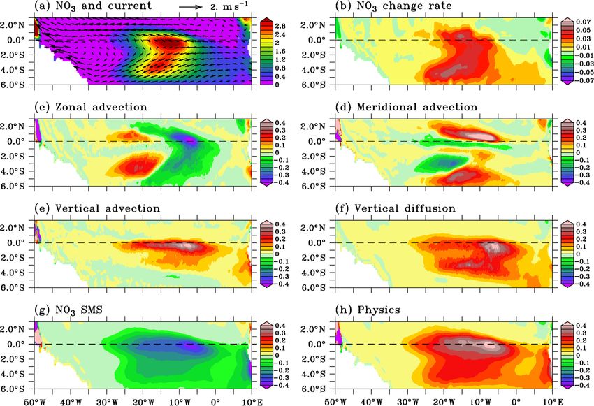
530                                               M.-H. Radenac et al.: Physical drivers of the nitrate seasonal variability

water supporting the phytoplankton growth in the euphotic        an offline nitrate transport model to examine the processes
layer. The advent of ocean color satellite measurements has      that drive nitrate to the surface. In their 2-year simulation,
made the monitoring of phytoplankton blooms possible and         surface nitrate concentration and biological production are
changed our vision of the equatorial variability. Using 1        more elevated in summer and decrease afterwards, although
year (March 1979–February 1980) of measurements from the         they remain higher in fall–early winter than in spring. In
Coastal Zone Color Scanner (CZCS), Monger et al. (1997)          summer, nitrate is brought to the EUC and euphotic layer
showed a higher chlorophyll value (more than 1 mg m−3 ) in       through vertical advection and reaches the surface through
October–December than in summer near 10◦ W. In contrast,         vertical diffusion. Christian and Murtugudde (2003) ran a 50-
during the first year of the Sea-viewing Wide Field-of-view      year-long coupled physical–biogeochemical model and un-
Sensor (SeaWiFS), a bloom was observed between May and           derlined the influence of the relative depth between the ni-
September, and the October–December chlorophyll values           tracline and the upwelling core on the nitrate variations. In
were low (Signorini et al., 1999). This suggests large inter-    spring, the surface nitrate is at its lowest because the up-
annual fluctuations of the equatorial productivity. Neverthe-    welling is weak and located above the nitracline. In con-
less, a semiannual cycle of surface chlorophyll emerges as       trast, surface nitrate peaks in summer when water is up-
illustrated by the ocean color archive for the period 1998–      welled from the subsurface in response to the basin-wide
2016 (Fig. 1a). This seasonal cycle is characterized by a        tilt of the thermocline/nitracline. More recently, Jouanno et
primary chlorophyll bloom in July–August between 20 and          al. (2011a) related processes responsible for SST changes
5◦ W and a shorter and weaker second bloom in Decem-             to the observed chlorophyll changes. They highlighted the
ber (Pérez et al., 2005; Grodsky et al., 2008; Jouanno et al.,   semiannual cycle of vertical mixing above the EUC core
2011a). Strong similarities between this seasonal cycle and      driven by the semiannual variation in the SEC. Maximum
the seasonal cycle of sea surface temperature (SST) suggest      vertical mixing and surface cooling occur concurrently in
that the same physical processes could control the supply of     summer while the impact of vertical mixing can be strongly
cool and nutrient-rich waters into the euphotic layer (Hisard,   damped by air–sea heat fluxes during the secondary cooling
1973; Oudot and Morin, 1987; Grodsky et al., 2008; Jouanno       in November–December. Because such a constraint does not
et al., 2011a).                                                  exist for surface chlorophyll, intensified vertical mixing and
   Investigations of the link between physical processes and     surface chlorophyll peak simultaneously in summer and in
biological production in the equatorial Atlantic were con-       November–December.
ducted using in situ measurements during oceanographic               The impact of tropical instability waves (TIWs) on the
cruises since the 1960s and satellite measurements since the     ecosystem of the Atlantic cold tongue was proposed by Mor-
1980s. The role of upwelling, vertical mixing, and variation     lière et al. (1994) and Menkes et al. (2002). Although there
in the depth of the thermocline and nitracline has been raised   is a debate about the influence of TIWs on the nutrient bud-
to explain the seasonal surface nitrate and chlorophyll in-      get in the equatorial Pacific (Strutton et al., 2001; Gorgues
crease. Hisard (1973) proposed that nutrient enrichment at       et al., 2005), no such study is available in the equatorial At-
5◦ W is mainly driven by the equatorial divergence in sum-       lantic where TIWs dominate the intraseasonal variability in
mer and persists until fall because of enhanced vertical mix-    the western and central basins and wind-forced waves domi-
ing. The enhancement of the vertical mixing during the cold      nate in the east (Athié and Marin, 2008).
season was associated with the strong vertical shear between         This study was motivated by observation of the nitrate ver-
the intensified South Equatorial Current (SEC) and the shal-     tical patterns during the low- and high-productivity seasons
lower Equatorial Undercurrent (EUC) by Voituriez and Herb-       by repeated in situ measurements along 10◦ W acquired dur-
land (1977). Considering oxygen and salinity distributions,      ing recent cruises and their link with the semiannual variabil-
Voituriez (1983) dismissed the influence of vertical mixing      ity of chlorophyll observed by ocean color satellites. Because
and emphasized the role of the thermocline/nitracline uplift.    cruise sampling prevents us from studying an entire seasonal
Oudot and Morin (1987) suggested that the equatorial diver-      cycle, a coupled physical–biogeochemical simulation is used
gence drove the summer nitrate enrichment and that its per-      to complement the nitrate and chlorophyll seasonal cycles
sistence until fall was supported by vertical mixing above       and to investigate the processes driving this seasonality. The
the EUC core whose nitrate concentration increased because       data sets we use and the coupled physical–biogeochemical
of the nitracline uplift. Monger et al. (1997) proposed that     model are described in Sect. 2. Previous studies have shown
upwelling was the driving mechanism of the summer and            that vertical processes (equatorial upwelling, vertical mixing,
fall nitrate increase and that its efficiency was modulated      and vertical motion of the nitracline) are involved in setting
by the relative depths of the EUC and nitracline. Grodsky et     the seasonal cycles of surface nitrate and chlorophyll. How-
al. (2008) stressed the role of the equatorial upwelling com-    ever, it is not clear how these vertical processes combine with
bined with the shoaling of the nitracline.                       horizontal processes to drive the bloom properties in terms of
   Few model-based studies have addressed the influence of       spatial extent and duration. This issue is investigated by an-
the ocean dynamics variability on the nutrient variability in    alyzing the model seasonal nitrate budget (Sect. 3). The role
the equatorial Atlantic. Loukos and Mémery (1999) used           of the variation in nitrate concentration in the EUC in the ni-

Biogeosciences, 17, 529–545, 2020                                                      www.biogeosciences.net/17/529/2020/
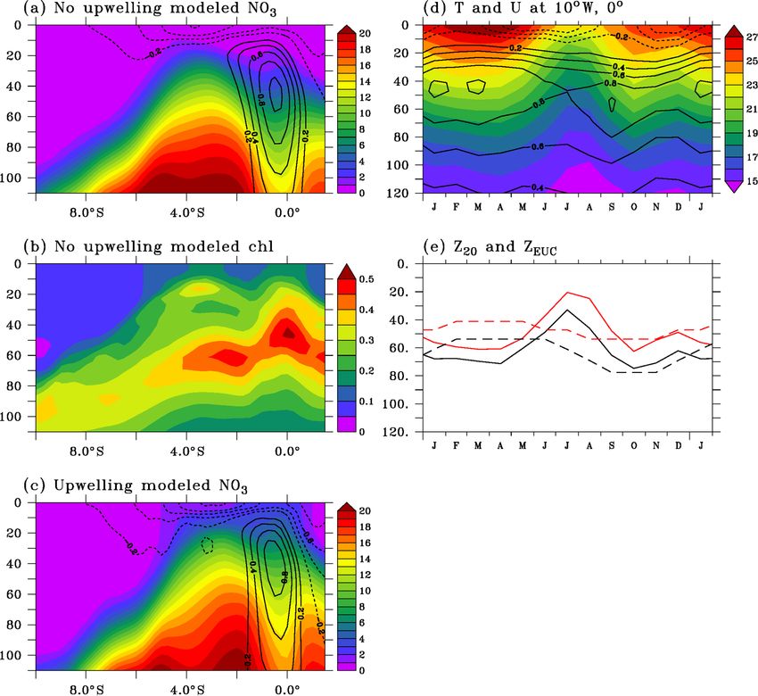
M.-H. Radenac et al.: Physical drivers of the nitrate seasonal variability                                                    531

trate budget in the euphotic layer and the impact of transient     mirrors the SST distribution (Fig. 1b). The minimum SST
processes such as TIWs and wind-forced waves are discussed         and maximum surface chlorophyll coincide and are located
in Sect. 4. Concluding remarks are presented in Sect. 5.           south of the Equator between 20 and 5◦ W. Chlorophyll and
                                                                   SST gradients are sharper on the northern side of the cold
                                                                   tongue than on the southern side. The surface chlorophyll
2     In situ and satellite observations                           value starts to increase in May (Fig. 1a), and the chloro-
                                                                   phyll maximum and SST minimum are found in July–August
2.1    Data sets
                                                                   and in December. The December peak is better defined with
We use in situ nitrate, chlorophyll, and acoustic Doppler          chlorophyll than with temperature. The surface chlorophyll
current profiler (ADCP) measurements collected during re-          is at its minimum in spring, and a secondary minimum oc-
peated transects along 10◦ W (Table 1) as part of the PIRATA       curs in October.
(Prediction and Research Moored Array in the Tropical At-             Vertical sections of nitrate, chlorophyll, and zonal cur-
lantic; Servain et al., 1998; Bourlès et al., 2008, 2019) and      rent along 10◦ W measured during the PIRATA cruises and
EGEE (Étude de la Circulation Océanique et de sa Variabilité       averaged separately in no-upwelling–low-productivity and
dans le Golfe de Guinée; Bourlès et al., 2007) programs. All       upwelling–high-productivity (Table 1) seasons are shown in
these data, along with information on their acquisition and        Fig. 2a–c. Results are close to the distributions during the
treatment, are available through their DOI (Bourlès, 1997;         cold and warm seasons described along 4◦ W in the 1970s
Bourlès et al., 2018a, c). The analysis is based on 13 transects   and 1980s (Voituriez and Herbland, 1977; Oudot, 1983;
with nitrate measurements between 2004 and 2014 and four           Monger et al., 1997) and along 10◦ W during the June and
transects with chlorophyll measurements corresponding to           September 2005 EGEE cruises (Nubi et al., 2016). During
the most recent French PIRATA cruises from 2011 to 2014.           the warm and low-productivity season, the low-chlorophyll
If we simply consider that upwelling conditions prevail when       (Fig. 2b) and nitrate-depleted (Fig. 2a) layer extends from the
nitrate concentration larger than 1 µmol L−1 is measured in        surface to 30 m between 1◦ N and 5◦ S and deepens south-
the upper 10 m between 2◦ S and 1◦ N, only two cruises fulfill     ward. Below, a nitracline ridge is observed between 2 and
these conditions (June 2005 and July 2009). Note that there        5◦ S. The deep chlorophyll maximum (DCM) is located in
are no chlorophyll measurements during the boreal summer           the upper nitracline and intensifies between 5◦ S and 2◦ N.
upwelling period.                                                  During the cold and high-productivity season, the nitracline
   Observations from a PIRATA ocean–atmosphere interac-            is uplifted and nitrate reaches the surface (Fig. 2c). The EUC
tion mooring and an ADCP mooring maintained at 10◦ W–              transports water with low-nitrate concentration compared to
0◦ N (Bourlès et al., 2018b) are also analyzed. We use             off-equatorial waters at the same depth (Fig. 2a, c; Oudot,
monthly temperature measurements available since Septem-           1983) for both seasons.
ber 1997 at 1, 5, 10, 20, 40, 60, 80, 100, 120, 140, 180, 300,        Previous studies have shown that the location of the ther-
and 500 m depth and daily ADCP current profiles available          mocline/nitracline relative to the EUC depth impacted the
every 5 m from 15 m to about 300 m depth between Decem-            efficiency of the upwelling (Monger et al., 1997; Christian
ber 2001 and March 2017.                                           and Murtugudde, 2003). Figure 2d illustrates the seasonal
   The climatology of surface chlorophyll is calculated from       vertical excursions of the thermocline and EUC as deduced
chlorophyll estimates at 25 km horizontal resolution of the        from the temperature and zonal current profiles measured at
monthly GlobColour merged product obtained from dif-               the 0◦ N, 10◦ W PIRATA mooring. Seasonal variations in the
ferent sensors and using the GSM (Garver, Siegel, Mari-            depth of the EUC core are small while the thermocline depth
torena) model described in Maritorena et al. (2010). Sensors       shows larger vertical movements. The thermocline is about
are Medium Resolution Imaging Spectrometer (MERIS),                20 m below the EUC core in April and about 30 m above in
SeaWiFS, Moderate Resolution Imaging Spectroradiome-               August, leading to variations in the properties of the EUC
ter (MODIS) Aqua, and the Visible and Infrared Im-                 water. The temperature is colder in the EUC in August than
ager/Radiometer Suite (VIIRS) when available.                      during spring. Likewise, nitrate is more elevated in the EUC
   The SST climatology is derived from the TropFlux data           in August than during spring (Oudot and Morin, 1987), as
set (Praveen Kumar et al., 2012). We use monthly SST maps          expected from the strong relationship between nitrate and
from 1979 to 2016 at 1◦ × 1◦ resolution between 30◦ S and          temperature in the nitracline of the cold tongue all year long
30◦ N.                                                             (Voituriez and Herbland, 1984).

2.2    Observed seasonal cycles

Correspondences between spatial patterns and seasonal cy-
cles of the surface chlorophyll and those of SST are illus-
trated in Fig. 1. In July–August, when the cold tongue ex-
pansion is the largest, the distribution of surface chlorophyll

www.biogeosciences.net/17/529/2020/                                                         Biogeosciences, 17, 529–545, 2020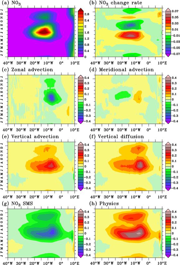
532                                                   M.-H. Radenac et al.: Physical drivers of the nitrate seasonal variability

Table 1. List of PIRATA (FR) and EGEE transects along 10◦ W and availability of NO3 , chlorophyll, and ADCP zonal current measurements.
Cruises used during the no-upwelling and upwelling periods are indicated in the last two columns.

                                     Dates              NO3      Chl   U     No-upwelling period     Upwelling period
                    FR12             February 2004        ×            ×              ×
                    FR14-EGEE1       June 2005            ×            ×                                     ×
                    EGEE2            September 2005       ×            ×                                     ×
                    FR15-EGEE3       June 2006            ×            ×                                     ×
                    EGEE4            November 2006        ×                                                  ×
                    FR17-EGEE5       June 2007            ×            ×                                     ×
                    EGEE6            September 2007       ×                                                  ×
                    FR19             July 2009            ×                           ×
                    FR20             September 2010       ×                                                  ×
                    FR21             May 2011             ×      ×     ×                                     ×
                    FR22             April 2012           ×      ×     ×                                     ×
                    FR23             May 2013             ×      ×     ×                                     ×
                    FR24             April 2014           ×      ×     ×                                     ×

Figure 1. Seasonal cycles averaged in the upwelling region (a) and mean distributions in July–August (b) of satellite chlorophyll (mg m−3 ;
colors) and observed SST (◦ C; contours). Data were averaged between 1.5◦ S and 0.5◦ N in (a). The SST contour interval is 0.5 ◦ C. Chloro-
phyll and SST climatologies are calculated over 1998–2015. See the data section for origin of data.

3     Coupled physical–biogeochemical simulation                        MERCATOR global reanalysis GLORYS2V4 (Storto et al.,
                                                                        2018) are used to force the model at the lateral boundaries.
3.1    Model description                                                   The physical model is coupled to the PISCES (Pelagic In-
                                                                        teraction Scheme for Carbon and Ecosystem Studies) bio-
                                                                        geochemical model (Aumont et al., 2015) that simulates the
A coupled simulation is used to describe the nitrate seasonal           biological production and the biogeochemical cycles of car-
cycle and the seasonal nitrate budget in the mixed and eu-              bon, nitrogen, phosphorus, silica, and iron. Two phytoplank-
photic layers. The physical component of the simulation is              ton classes (nanophytoplankton and diatoms) differ by their
based on the NEMO (Nucleus for European Modeling of the                 silicate and iron requirements. The two zooplankton com-
Ocean; Madec and the NEMO team, 2016) numerical code.                   partments (nanozooplankton and mesozooplankton) feed on
We use the regional configuration described in Hernandez                the two phytoplankton classes. The model also includes three
et al. (2016, 2017) that covers the tropical Atlantic between           nonliving compartments (dissolved organic matter and small
35◦ S and 35◦ N and from 100◦ W to 15◦ E. The resolution                and large sinking particles). The biogeochemical model is
of the horizontal grid is 1/4◦ and there are 75 vertical levels,        initialized and forced at the lateral boundaries with dissolved
24 of which are in the upper 100 m layer. The depth inter-              inorganic carbon, dissolved organic carbon, alkalinity, and
val ranges from 1 m at the surface to about 10 m at 100 m               iron obtained from stabilized climatological 3-D fields of the
depth. Interannual atmospheric fluxes of momentum, heat,                global standard configuration ORCA2 (Aumont and Bopp,
and freshwater are derived from the DFS5.2 product (Dussin              2006) and nitrate, phosphate, silicate, and dissolved oxygen
et al., 2016) using bulk formulae from Large and Yeager
(2009). Temperature, salinity, current, and sea level from the

Biogeosciences, 17, 529–545, 2020                                                              www.biogeosciences.net/17/529/2020/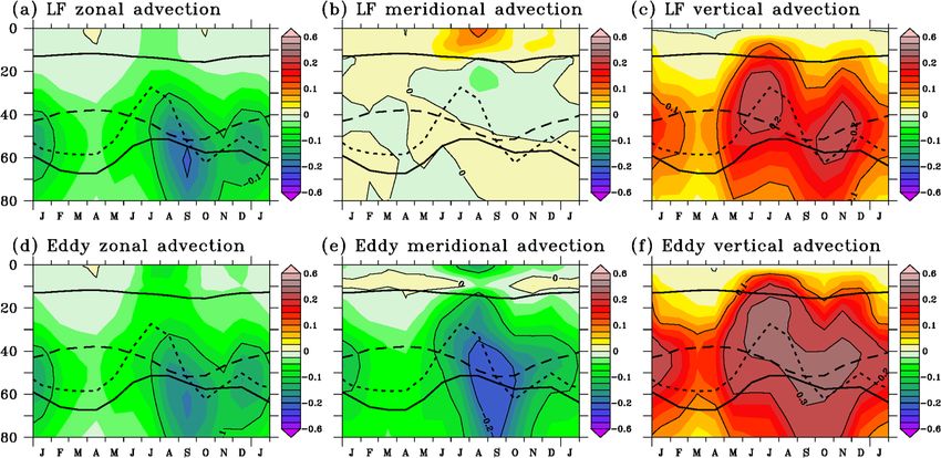
M.-H. Radenac et al.: Physical drivers of the nitrate seasonal variability                                                                 533

Figure 2. (a, c) Observed nitrate (µmol L−1 ) and chlorophyll (mg m−3 ; (b) distributions along 10◦ W during low-productivity (a, b) and
high-productivity (c) conditions. Zonal velocity is overlaid on nitrate distribution. (d) Seasonal cycles of temperature (colors; ◦ C) and zonal
current (contours; m s−1 ) at the 0◦ N, 10◦ W mooring. Velocity contour interval is 0.2 m s−1 ; the 0 m s−1 contour has been removed.

from the World Ocean Atlas observation database (WOA;                        We estimate the low- and high-frequency contributions to
Garcia et al., 2010).                                                     the advection terms by separating off-line each advection
   The model is integrated from 1993 to 2015 and monthly                  term into low-frequency and submonthly components:
averages for the period 1995 to 2015 are analyzed. Such short
spin-up is justified by the fast adjustment of the equatorial                  ∂NO3      ∂NO3      ∂NO03
dynamics and the main focus of the study which is on the                  −u        = −u      − u0       .                                  (2)
                                                                                ∂x        ∂x        ∂x
upper ocean variability.
   The three-dimensional nitrate balance solved in the model              The left-hand-side term is the monthly average of zonal ad-
reads as follows:                                                         vection. On the right-hand side, the first term is the monthly
∂NO3           ∂NO3      ∂NO3        ∂NO3                                 zonal advection calculated from monthly averages of zonal
       = −u           −v        −w                                        current (u) and nitrate concentrations (NO3 ). The second
  ∂t            ∂x        ∂y           ∂z
                       ∂

                               ∂NO3
                                                                         term is the eddy advection term. It includes all the sub-
       + Dl (NO3 ) +        Kz          + SMS,            (1)             monthly advection contributions which, in this region, may
                       ∂z        ∂z
                                                                          include influences of inertia–gravity waves, mixed Rossby–
in which NO3 is the model nitrate concentration, (u, v, w)                gravity waves, Kelvin waves, and eddies or tropical insta-
are the velocity components, Dl (NO3 ) is the lateral diffusion           bility waves (e.g., Athié et al., 2009; Jouanno et al., 2013).
operator, and Kz is the vertical diffusion coefficient for trac-          It is calculated as the residual between the total and mean
ers. The first three terms on the right-hand side are the zonal,          zonal advection. Meridional and vertical advection are de-
meridional, and vertical advection; the fourth and fifth terms            composed in the same way. Such decomposition has been
are the lateral and vertical diffusions. The last term, called            used to estimate the eddy contribution to SST budget in the
“source minus sink” (SMS), is the nitrate change rate due to              Pacific mixed layer (Vialard et al., 2001) and oxygen advec-
biogeochemical processes which include uptake by nanophy-                 tion in the Arabian Sea (Resplandy et al., 2012).
toplankton and diatoms, nitrification, denitrification, and ni-              We use the method described in Vialard and Delecluse
trogen fixation. The different terms are computed online and              (1998) to investigate nitrate budgets in the mixed layer and
averaged over 1-month periods.                                            in the euphotic layer. An entrainment term appears when in-

www.biogeosciences.net/17/529/2020/                                                                    Biogeosciences, 17, 529–545, 2020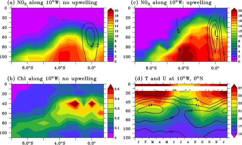
534                                                M.-H. Radenac et al.: Physical drivers of the nitrate seasonal variability

tegrating Eq. (1) over a time-varying layer:                      RATA mooring at 0◦ N, 10◦ W were used to calculate the
∂hNO3 i

                  ∂NO3

                               ∂NO3

                                             ∂NO3
                                                                 climatology shown in Fig. 4d. The amplitude and phase of
          =− u            − v          − w                        the seasonal cycles of modeled temperature and zonal cur-
    ∂t             ∂x            ∂y            ∂z
                                                                rent compare well, although the simulated temperature and
                           1      ∂NO3                            current vertical structures are shallower than observed. The
          + hDl (NO3 )i +     Kz                + hSMSi
                           h        ∂z     z=−h                   depths of the 20 ◦ C isotherm (Z20) and of the EUC core
            1 ∂h                                                 (ZEUC) are 12 and 16 m shallower than observed, respec-
          −        hNO3 i − NO3z=−h ,                       (3)   tively (Fig. 4e). However, the relative position of Z20 and
            h ∂t
where brackets indicate the vertical average over the layer       ZEUC is correctly reproduced. The simulated nitrate con-
depth h. The last term arises from time variations in the inte-   centration at ZEUC (not shown) is less than 2 µmol L−1 in
gration depth h. This term is often referred to as entrainment    spring and rises to nearly 9 µmol L−1 in August, in agree-
at the base of the layer (e.g., Vialard and Delecluse, 1998)      ment with observations at 4◦ W (Oudot and Morin, 1987). In
and computed as a residual of the other terms of Eq. (3).         the 20 m surface layer, the model captures the weakening of
Here we verified that this term is small and we choose not        the SEC in January–February and September–October well
to show it. The mixed-layer depth is computed as the depth        (Okumura and Xie, 2006; Ding et al., 2009; Habasque and
where the density is 0.03 kg m−3 higher than the 10 m den-        Herbert, 2018).
sity (de Boyer Montégut et al., 2004) and the depth of the
euphotic layer is the depth where the surface photosyntheti-
cally available radiation (PAR) is reduced to 1 % (Morel and      4     The modeled nitrate seasonal cycle
Berthon, 1989). The contribution of lateral diffusion to the
nitrate budgets in both layers is weak and is not shown.          The good agreement between the observed and simulated
                                                                  patterns and seasonal variations in chlorophyll and nitrate
3.2   Evaluation of the modeled seasonal cycle                    makes the model a relevant tool to investigate the seasonal
                                                                  nitrate budget. Understanding variations in the surface pro-
The climatology of the simulated surface chlorophyll cal-         ductivity requires identification of processes below the mixed
culated over the same period (1998–2015) as observations          layer. So in this section, processes driving the seasonal varia-
(Fig. 1) is shown in Fig. 3. The model reproduces the pat-        tions in nitrate are presented in the mixed layer, but also down
tern and semiannual variability of surface chlorophyll in the     to the base of the euphotic layer. We focus on the 1.5◦ S–
equatorial cold tongue. The simulated chlorophyll maximum         0.5◦ N, 20–5◦ W region where the surface chlorophyll values
is shifted about 5◦ east of the chlorophyll maxima observed       are the largest.
by satellite. The model surface chlorophyll is also slightly
higher than observed east of the equatorial chlorophyll max-      4.1    Nitrate budget in the mixed layer
imum.
   The meridional sections of modeled nitrate and chloro-         In the equatorial Atlantic, the seasonal variations in chloro-
phyll along 10◦ W presented in Fig. 4a–c have been cal-           phyll are thought to be primarily related to seasonal vari-
culated using fields coincident with observed sections in         ability of the nitrate input (Voituriez and Herbland, 1977;
Fig. 2a–c. The model properly reproduces the main fea-            Loukos and Mémery, 1999). This is illustrated well by the
tures such as the nitracline uplift around 3◦ S and the low-      seasonal cycle of nitrate built from 21 years of simulation
nitrate signature of the EUC (Fig. 4a, c). However, the sim-      (1995–2015) in Fig. 5a, which closely matches the seasonal
ulated nitrate has a positive bias that can reach 5 µmol L−1      variability of the model (Fig. 3b) and satellite chlorophyll
in the nitracline in the 5–2◦ S region. In the equatorial         (Fig. 1a).
zone, the model nitrate is slightly overestimated (less than         The mixed-layer nitrate concentration at the Equator
1 µmol L−1 ) above the 5 µmol L−1 nitrate isoline (which is       shows large and coherent variations between 30◦ W and 0◦ E
close to the 20 ◦ C isotherm depth) and slightly underesti-       (Fig. 5a). This central equatorial variability does not seem
mated (about 1 µmol L−1 ) below. The nitrate-depleted sur-        to be directly connected with mixed-layer nitrate input along
face layer is about 10 m shallower in the simulation than         the African coast, in agreement with the chlorophyll behavior
in the observations. In the equatorial zone, the position of      in the equatorial Atlantic deduced from satellite data (Grod-
the simulated DCM in the upper nitracline is in agreement         sky et al., 2008). Four phases emerge from the nitrate sea-
with observations while its magnitude is more elevated by         sonal evolution in the mixed layer of the central equato-
about 0.1 mg m−3 (Fig. 4b). Too high simulated chlorophyll        rial Atlantic: a nitrate increase between April and July, a
is found up to the surface where the concentration is about       decrease between August and October, a rapid increase in
0.15 mg m−3 at the Equator instead of 0.1 mg m−3 in the ob-       November, and a secondary decrease starting in December
servations.                                                       (Fig. 5b). This temporal pattern results from the imbalance
   Simulated profiles of temperature and zonal current coin-      between physical processes (Fig. 5h) that brings nitrate into
cident with available observed profiles (Fig. 2d) at the PI-      the mixed layer and nitrate uptake by the biological activity

Biogeosciences, 17, 529–545, 2020                                                       www.biogeosciences.net/17/529/2020/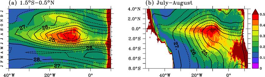
M.-H. Radenac et al.: Physical drivers of the nitrate seasonal variability                                                        535

Figure 3. Seasonal cycle averaged in the upwelling region (a) and mean distribution in July–August (b) of simulated surface chlorophyll
(mg m−3 ). Data were averaged between 1.5◦ S and 0.5◦ N in (a). The climatology is calculated over 1998–2015.

(Fig. 5g). Unlike the negligible contribution of vertical ad-         4.2   Nitrate budget in the euphotic layer
vection in the temperature budget in the mixed layer of the
equatorial Atlantic (Jouanno et al., 2011b), both vertical ad-
vection (Fig. 5e) and vertical diffusion (Fig. 5f) contribute         In this section, we examine how, in addition to processes in
to nitrate inputs in the mixed layer. Variations in zonal ad-         the mixed layer, variations in nitrate below the mixed-layer
vection drive variations in horizontal advection (Fig. 5c, d)         impact variations in surface nitrate and, in turn, chlorophyll.
that acts to bring some low-nitrate water to the cold tongue          Also, variations in the euphotic layer where the biological
area during most of the year. The main peak occurs in July–           production takes place allow better explanation of the tran-
August and a secondary peak occurs in December. Horizon-              sition between the low- and high-productivity seasons. The
tal advection is close to zero in February–May.                       seasonal cycles of chlorophyll, nitrate, and the main pro-
   In Fig. 6, we show the regional distribution of the dif-           cesses involved in nitrate change in the 1.5◦ S–0.5◦ N, 20–
ferent terms of the nitrate balance in July, when the nitrate         5◦ W region from the surface to 80 m are shown in Fig. 7.
supply to the mixed layer by physical processes and nitrate           Depths of the mixed layer, of the euphotic layer, and of the
uptake are at their maximum. During this period, the biolog-          EUC core are overlaid. The depth of the thermocline core
ical sink is not efficient enough to offset the physical supply       is represented by the 20 ◦ C isotherm depth. The separated
and the surface nitrate (Fig. 6a) shows a maximum between             low-frequency and submonthly contributions to the advec-
1.5◦ S and 0.5◦ N from 20 to 5◦ W at the location of maxi-            tion terms are presented in Fig. 8.
mum vertical input through advection (Fig. 6e) and diffusion             The semiannual cycle of chlorophyll described in the
(Fig. 6f) and biological sink (Fig. 6g). Advection of nitrate-        mixed layer is also visible in the entire euphotic layer
poor water from the east (Fig. 6c) and meridional advection           (Fig. 7a). The seasonal cycle of the depth of the simulated
(Fig. 6d) slightly counteract the vertical nitrate supply near        DCM is in agreement with observations (Monger et al.,
the Equator. Off the Equator, meridional advection acts to            1997). It is located near the thermocline core between 50 and
spread the upwelled nitrate-rich water poleward along the             60 m in spring, rises toward the surface at the same time as
northern boundary of the nitrate-rich patch and, to a lesser ex-      the thermocline core in summer, sinks in early fall, and rises
tent, along the southern boundary where the nitrate gradient          again in November. In February–April, chlorophyll values
is weaker. This may contribute to the meridional extension of         are low in the nitrate-depleted surface layer as in oligotrophic
the observed (Fig. 1b) and model (Fig. 3a) chlorophyll dis-           ecosystems. The semiannual variations in chlorophyll in the
tribution.                                                            euphotic layer are closely associated with semiannual varia-
   The scenario leading to the December secondary nitrate             tions in nitrate (Fig. 7b).
maximum in the mixed layer is close to the boreal summer                 The nitrate change rate is at a maximum at the base of the
nitrate evolution, except that the duration of the processes is       euphotic layer near the EUC core (Fig. 7c). Its semiannual
shorter (about 1 month long), their magnitudes are weaker,            cycle can be seen as an interplay between the physical sup-
and they span a narrower longitudinal range (Fig. 5). Be-             ply (Fig. 7i) and the biological sink (Fig. 7h). Physical pro-
tween the summer and December nitrate maxima, vertical                cesses mostly bring nitrate into the euphotic layer with max-
processes strongly decrease (Fig. 5c, f) and sustain less ni-         imum input in the mixed layer in May–August and below the
trate supply in the mixed layer, allowing the biological sink         mixed layer in November. In contrast, nitrate is consumed by
(Fig. 5g) to prevail over the physical input (Fig. 5h).               the biological activity in the euphotic layer and remineralized
                                                                      below. Physical supply is stronger than biological loss dur-
                                                                      ing the main peak of the nitrate change rate in May–July and

www.biogeosciences.net/17/529/2020/                                                             Biogeosciences, 17, 529–545, 2020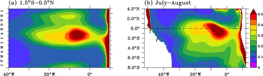
536                                                     M.-H. Radenac et al.: Physical drivers of the nitrate seasonal variability

Figure 4. (a, c) Simulated nitrate (µmol L−1 ) and chlorophyll (mg m−3 ; b) distributions along 10◦ W during low-productivity (a, b) and
high-productivity (c) conditions. Zonal velocity is overlaid on nitrate distribution. (d) Seasonal cycles of temperature (colors; ◦ C) and zonal
current (contours; m s−1 ) at 0◦ N, 10◦ W. Velocity contour interval is 0.2 m s−1 ; the 0 m s−1 contour has been removed. (e) Observed (black)
and simulated (red) depths of the 20 ◦ C isotherm (full line) and of the EUC core (dashed line) at 0◦ N, 10◦ W.

during the short second peak in November; biological losses               strengthen. The maximum vertical advection is located near
prevail over the physical supply in August–October and in                 the layer of maximum vertical nitrate gradient, close to the
December–January. The nitrate supply in November suggests                 depth of the 20 ◦ C isotherm, and it occurs when the vertical
that the observed and simulated elevated chlorophyll values               velocity is strong (July and November). Vertical advection
in December result from a second chlorophyll bloom and                    of nitrate-rich water at the base of the mixed layer favors
not from a persistence of elevated nitrate and chlorophyll                the intensified vertical diffusion in summer and November–
concentrations following the summer bloom (Hisard, 1973;                  December (Fig. 7g), with an acceleration of the SEC which
Oudot and Morin, 1987).                                                   increases the vertical shear with the EUC and, in turn, in-
   Vertical advection always brings nitrate into the euphotic             creases the vertical mixing in the mixed layer (Jouanno et al.,
layer (Fig. 7f). It drives the main nitrate increase in May–              2011b). Both the low-frequency (Fig. 8c) and eddy (Fig. 8f)
July and the secondary one in November when easterly winds                advection contribute to the nitrate supply through vertical ad-

Biogeosciences, 17, 529–545, 2020                                                                  www.biogeosciences.net/17/529/2020/
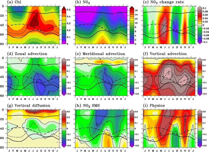
M.-H. Radenac et al.: Physical drivers of the nitrate seasonal variability                                                                    537

Figure 5. Seasonal cycle of modeled (a) surface nitrate (µmol L−1 ), (b) nitrate change rate, (c) zonal advection, (d) meridional advection,
(e) vertical advection, (f) vertical diffusion, (g) nitrate source minus sink, and (h) physical processes averaged in 1.5◦ S–0.5◦ N in the mixed
layer. Tendency units are micromoles per liter per day. Note that the color scale of nitrate change rate is different from the color scale of other
tendencies. Climatology has been calculated between 1995 and 2015.

www.biogeosciences.net/17/529/2020/                                                                      Biogeosciences, 17, 529–545, 2020
538                                                    M.-H. Radenac et al.: Physical drivers of the nitrate seasonal variability

Figure 6. Maps of (a) nitrate, (b) nitrate change rate, (c) zonal advection, (d) meridional advection, (e) vertical advection, (f) vertical
diffusion, (g) nitrate source minus sink, and (h) physical processes averaged in the mixed layer in July. The mean current in the mixed layer
is superimposed in (a). Note that color scale in (b) is different from the color scale in (c)–(h). Nitrate units are micromoles per liter and
tendency units are micromoles per liter per day.

vection, especially in the upper EUC between June and De-                tion (Fig. 8b) reveals the influence of the equatorial cell: the
cember. The eddy advection is more sustained than the low-               northward transport of nitrate-rich upwelled water dominates
frequency advection.                                                     the meridional advection in the mixed layer on average in the
   Below the mixed layer, horizontal advection (Fig. 7d,                 1.5◦ S–0.5◦ N, 20–5◦ W region.
e) removes nitrate all year long. It drives the strong ni-
trate loss in August–September and the lesser nitrate loss in
December–January (Fig. 7c) when the contributions of both                5     Discussion
zonal (Fig. 7d) and meridional (Fig. 7e) advection are the
largest. The contribution of the low-frequency zonal advec-              Observations and the model used in this study show semi-
tion (Fig. 8a) compares to that of the eddy advection (Fig. 8d)          annual cycles of chlorophyll and nitrate. The model further
while the eddy signal (Fig. 8e) controls the meridional advec-           shows that they are sustained by semiannual variations in
tion. Negative low-frequency zonal and meridional advection              processes in the euphotic layer. Changes of nitrate proper-
indicate the transport of low-nitrate water from the west by             ties in the EUC and intraseasonal processes are involved in
the EUC and from the north by the low-frequency southward                shaping the seasonal cycle of nitrate supply and losses.
component of the subsurface current (Perez et al., 2014). In
the mixed layer, zonal advection acts to decrease the nitrate            5.1    Variability of nitrate in the Equatorial
concentration, and meridional advection is a weak source of                     Undercurrent
nitrate. The low-frequency advection of nitrate poor water
from the east is the largest where the zonal nitrate gradi-              Upwelled water in the central basin originates in the upper
ent is the strongest. The low-frequency meridional advec-                part of the EUC (Fig. 7f). The EUC waters mainly origi-
                                                                         nate in the very oligotrophic ecosystem of the south sub-

Biogeosciences, 17, 529–545, 2020                                                                www.biogeosciences.net/17/529/2020/
M.-H. Radenac et al.: Physical drivers of the nitrate seasonal variability 539 Figure 7. Seasonal cycle of vertical profiles of (a) chlorophyll, (b) nitrate, (c) nitrate change rate, (d) zonal advection, (e) meridional advection, (f) vertical advection, (g) vertical diffusion, (h) nitrate source minus sink, and (i) physical processes averaged in 1.5◦ S–0.5◦ N, 20–5◦ W. Chlorophyll units are milligrams per cubic meter, nitrate units are micromoles per liter, and tendency units are micromoles per liter per day. Tendency contours are every 0.1 µmol L−1 d−1 . The depths of the mixed layer (upper solid line), of the euphotic layer (lower solid line), of the EUC core (dashed line), and of the 20 ◦ C isotherm (dotted line) are indicated. Note that color scale in (c) is different from the color scale in (d)–(i). tropical gyre (Oudot, 1983; Blanke et al., 2002; Hazeleger teractions between wind-forced Kelvin waves and boundary- et al., 2003; Aiken et al., 2017). Waters are transported west- reflected Rossby waves (Merle, 1980; Ding et al., 2009). This ward, feed the North Brazil Undercurrent (NBUC), and are adjustment conditions the depth of the thermocline and asso- entrained within the North Brazil Current retroflection before ciated nitracline that varies from 60 m in spring to about 20 m entering the EUC. A small fraction of water also originates in in July–August while the upwelling core remains in the up- the North Equatorial Current (Bourlès et al., 1999; Hazeleger per part of the EUC, at 20–30 m, all year long (Fig. 4e). The et al., 2003). Therefore, this may explain that water trans- smallest vertical supply (Fig. 7f) occurs when the nitracline ported eastward by the EUC has relatively low nitrate con- is well below the weak upwelling core in spring. In May– centrations compared to nearby north and south water masses July and November, the vertical velocity is strong and the (Fig. 3a, c) in agreement with in situ measurements (Oudot, nitracline gets closer to the upwelling core, allowing vertical 1983). This relatively low-nitrate water is upwelled toward advection to increase. the surface layer along the Equator. The annual shoaling of the thermocline in the western Seasonal changes of the nitrate concentration in the EUC basin associated with the semiannual shoaling in the cen- in the central equatorial basin are closely related to the sea- tral basin leads to a strong zonal slope of the thermocline sonal nitracline shoaling (Oudot and Morin, 1987). The semi- depth in July–September and December–January (Ding et annual cycle of the nitracline depth follows the basin-wide al., 2009) and also of the nitracline. During these periods of adjustment of the thermocline to the wind forcing via in- time, the resulting strongly negative zonal advection (Fig. 7d) www.biogeosciences.net/17/529/2020/ Biogeosciences, 17, 529–545, 2020
540                                                     M.-H. Radenac et al.: Physical drivers of the nitrate seasonal variability

Figure 8. Seasonal cycle of vertical profiles of low-frequency (LF; a, b, c) and eddy (d, e, f) zonal advection (a, d), meridional advection (b,
e), and vertical advection (c, f). Tendency contours are every 0.1 µmol L−1 d−1 . The depths of the mixed layer (upper solid line), of the
euphotic layer (lower solid line), of the EUC core (dashed line), and of the 20 ◦ C isotherm (dotted line) are indicated.

in the EUC underlines the efficiency of the EUC in reduc-                 origins as temperature modulations observed at periods be-
ing the local nitrate concentrations. Nitrate removal by zonal            tween 10 and 50 d in the cold tongue (Marin et al., 2009;
advection in the EUC contributes to decrease the vertical ni-             de Coëtlogon et al., 2010; Jouanno et al., 2013; Herbert and
trate gradient, which, associated with a reduced vertical ve-             Bourlès, 2018). TIWs are observed west of 10◦ W at periods
locity, leads to moderate vertical nitrate supply in August–              between 20 and 50 d (Jochum et al., 2004; Athié and Marin,
September. At that time of the year, physical processes drive             2008; Jouanno et al., 2013). They are active in boreal sum-
reduced nitrate supply in the upper part of the euphotic layer            mer, decrease in fall, emerge again at the end of the year
and nitrate removal in its deeper part (Fig. 7i).                         with lesser intensity than in summer, and disappear in spring
   The seasonal nitrate supply in the center of the equato-               (Jochum et al., 2004; Caltabiano et al., 2005; Perez et al.,
rial Atlantic is supported by vertical processes and strongly             2019). East of 10◦ E, the impacts of wind-forced equatorial
modulated by losses through horizontal advection in the EUC               waves superimpose at different frequencies (Houghton and
linked to the semiannual thermocline uplift of the nitracline.            Colin, 1987; Athié et al., 2008; de Coëtlogon et al., 2010;
Variations in the nitrate concentration in the source waters              Jouanno et al., 2013; Herbert and Bourlès, 2018): Kelvin
of the NBUC may be another driver of nitrate variations in                waves at periods between 25 and 40 d, mixed Rossby–gravity
the EUC as suggested by White (2015), who finds that varia-               waves between 15 and 20 d, and inertia–gravity waves be-
tions in temperature in the NBUC contribute to variations in              tween 5 and 11 d.
the cold tongue SST 6 to 8 months later. Changes along the                   Considering the upper 20 m in the equatorial Atlantic,
EUC pathway (meridional circulation in the tropical cells, el-            Jochum et al. (2004) found that the annual meridional advec-
evation of the nitracline in the west, intraseasonal processes)           tive heat flux associated with TIWs was nearly offset by the
may also impact horizontal and vertical nitrate gradient and              vertical advective heat flux. In contrast, Peter et al. (2006)
the rates of supply and removal of nitrate in the central equa-           attributed the warming in the mixed layer induced by eddy
torial Atlantic. This deserves further attention.                         horizontal advection between 30 and 5◦ W to TIWs because
                                                                          of strong southward heat transport. In the Pacific Ocean, the
5.2   Intraseasonal processes                                             compensation between the TIW horizontal and vertical heat
                                                                          advection in the mixed layer was also suggested by Vialard
On average in the 1.5◦ S–0.5◦ N, 20–5◦ W region, our model                et al. (2001). However, Menkes et al. (2006) found that the
results show that horizontal eddy advection is responsible for            vertical advection associated with TIWs was low and their
nitrate decrease, especially in August–September, and that                effect was to warm the Pacific cold tongue in the upper
vertical eddy advection supplies the euphotic layer with ni-              200 m. Mixed Rossby–gravity waves, inertia–gravity waves,
trate. The intraseasonal nitrate variations may have the same

Biogeosciences, 17, 529–545, 2020                                                                  www.biogeosciences.net/17/529/2020/
M.-H. Radenac et al.: Physical drivers of the nitrate seasonal variability 541 and Kelvin waves are believed to contribute to cooling the zonal advection while eddy meridional advection strongly Atlantic cold tongue through both northward advection of decreases (not shown). Drawing again an analogy between cold tongue water and vertical mixing (Houghton and Colin, temperature and nitrate, the nitrate decrease through zonal 1987; Marin et al., 2009; Jouanno et al., 2013), although no advection could be attributed to Kelvin waves. In contrast, calculations of the heat budget were done. no nitrate increase through meridional advection is simulated The coincidence of high chlorophyll concentrations with as would be expected from mixed Rossby–gravity, inertia– meridional oscillations of currents associated with an anti- gravity, and Kelvin waves that cool the mixed layer. The con- cyclonic eddy observed during a summer cruise in the equa- clusion on the nature of intraseasonal processes that affect torial Atlantic (Morlière et al., 1994) strongly suggests that the nitrate budget east of 10◦ W is not straightforward. One TIWs may also influence ecosystems. This was further set- reason could be that the low-frequency signal captures part tled with synoptic observations of physical (temperature, of the Kelvin-wave-induced variability as there is no sharp salinity, current) and ecosystem (nitrate, chlorophyll, zoo- cutoff at 30 d in the spectrum of Kelvin waves (Athié and plankton, micronekton) tracers in a tropical instability vor- Marin, 2008; Athié et al., 2009; Jouanno et al., 2013). An- tex (Menkes et al., 2002): their horizontal and vertical struc- other reason would be related to the different distribution of tures were highly coherent. As for the heat budget, the impact temperature and nitrate in the mixed layer because the ni- of TIWs on biological production is debated, at least in the trate concentration rapidly drops to zero east of 10◦ W while equatorial Pacific Ocean. Gorgues et al. (2005) show that the a temperature gradient persists in this simulation. effect of TIWs is to lower the chlorophyll concentration near On an annual average, nitrate is supplied by intraseasonal the Equator, because the iron loss through horizontal advec- advection because eddy-induced vertical advection exceeds tion exceeds iron supply by vertical advection while Strutton horizontal advection. It represents a significant contribution et al. (2001) show that chlorophyll increases because of en- to the nitrate budget in the central equatorial Atlantic: about hanced upwelling. As far as we know, no study shows the 35 % of the advective nitrate input in the mixed layer and possible impact of TIWs and other intraseasonal waves on about 45 % in the euphotic layer. It differs from the overall nitrate budget in the Atlantic Ocean. warming contribution of TIWs to the SST budget of the equa- The more elevated surface chlorophyll concentrations are torial Pacific cold tongue showed by Menkes et al. (2006). found in the 1.5◦ S–0.5◦ N, 20–5◦ W zone which is affected This warming contribution reflects the impact of horizontal by TIWs and Kelvin waves in the 20–50 d period range and advection as TIW-induced vertical advection is negligible. by mixed Rossby–gravity and inertia–gravity waves at higher As far as horizontal eddy advection is concerned, the warm- frequency. In this study, a 1-month threshold separates the ing effect of zonal and meridional advection in the Pacific is eddy signal from the low-frequency signal. So, the impacts consistent with the nitrate removal by zonal and meridional of mixed Rossby–gravity and inertia–gravity waves and part advection in the Atlantic. of the variability associated with TIWs and Kelvin waves at This simulation was initially designed to study the large- periods shorter than 1 month enter the eddy advection terms. scale processes and it does not allow conclusions about the The part of the TIW and Kelvin wave signal with longer pe- role of the different intraseasonal processes. However, our riods is included in the low-frequency advection terms. results strongly suggest that large-scale processes cannot to- Several intraseasonal processes should contribute to the tally explain the seasonal evolution of the nitrate budget. Pre- seasonal nitrate loss through eddy horizontal advection and vious studies (e.g., Athié et al., 2009; Jouanno et al., 2013) nitrate input through eddy vertical advection in the mixed show that this model reproduces the level of energy of the layer and in the euphotic layer in the 1.5◦ S–0.5◦ N, 20–5◦ W TIWs and their equatorial signature in terms of sea surface region. In this simulation, nitrate loss in the mixed layer west temperature. It suggests that their contribution to the nitrate of 10◦ W is driven by eddy meridional advection and by eddy budget is well resolved, but this cannot be fully demonstrated zonal advection to a lesser extent (not shown). As the hori- from an observational basis since the only available nitrate zontal and vertical patterns of temperature and nitrate in a data in the cold tongue area are from the PIRATA cruises tropical instability vortex are close (Menkes et al., 2002), the which do not provide high-frequency information on the nu- advection of nitrate anomaly by eddy zonal and meridional trient distribution. A dedicated study allowing better separa- currents could drive nitrate losses by eddy zonal and merid- tion of the large-scale and eddying signals is needed in order ional advection in the same way as the advection of anoma- to identify the nature of intraseasonal processes at work and lous temperature by anomalous currents drives a mixed-layer their impact on the seasonal nitrate budget in the Atlantic warming close to the Equator. By analogy with TIW-induced cold tongue area. warming (Vialard et al., 2001; Peter et al., 2006; Menkes et al., 2006), TIWs could be a strong contributor to the nitrate eddy term. Nitrate loss by eddy horizontal advection is also 6 Conclusion consistent with iron loss associated with TIWs in the equato- rial Pacific (Gorgues et al., 2005). East of 10◦ W, the nitrate We described and analyzed the seasonal cycle of nitrate and removal through eddy horizontal advection is driven by eddy the associated physical processes in the Atlantic cold tongue www.biogeosciences.net/17/529/2020/ Biogeosciences, 17, 529–545, 2020
542                                                     M.-H. Radenac et al.: Physical drivers of the nitrate seasonal variability

region using in situ and satellite data and a coupled physical–         MHR conducted the analysis with help from JJ. MHR wrote the
biogeochemical simulation. The model reproduces the hori-               manuscript with contributions from all coauthors.
zontal and vertical patterns of chlorophyll observed in the
studied area and its semiannual cycle. Nitrate required for
the phytoplankton growth is supplied by vertical processes.             Competing interests. The authors declare that they have no conflict
The main supply period occurs from May to July and a sec-               of interest.
ondary supply also occurs in November. In between, nitrate is
removed by horizontal advection in August–September and
during the secondary loss event in December–January. We                 Acknowledgements. We thank the IRD IMAGO team, Pierre Rous-
                                                                        selot (ADCP), François Baurand (nutrients), and Sandrine Hillion
draw attention to the potential roles of nitrate variations in
                                                                        (chlorophyll), for collecting, validating, and making available the
the EUC and of intraseasonal processes in the seasonal ni-              French PIRATA cruise measurements, along with Jacques Grelet,
trate budget.                                                           Fabrice Roubaud, and other engineers and technicians of the PI-
   Ding et al. (2009) put forward the presence of a basin               RATA program for maintaining the ocean–atmosphere interaction
mode that explains semiannual changes of sea surface height             buoys and ADCP moorings. We acknowledge the GlobColour
(SSH) gradient. Our results show how the thermocline and                and TropFlux projects for sharing the freely available data we
nitracline uplift affects the zonal nitrate gradient in the EUC         use. GlobColour data have been developed, validated, and dis-
and thus how it influences nitrate removal by horizontal ad-            tributed by ACRI-ST, France. The TropFlux data are produced
vection and then vertical supply. Changes of the nitrate con-           under a collaboration between Laboratoire d’Océanographie: Ex-
centration in the source water within the NBUC may also                 périmentation et Approches Numériques (LOCEAN) from Insti-
impact nitrate changes in the center of the basin. A dedi-              tut Pierre Simon Laplace (IPSL, Paris, France) and the National
                                                                        Institute of Oceanography/CSIR (NIO, Goa, India) and supported
cated study of nitrate variations in the EUC and associated
                                                                        by Institut de Recherche pour le Développement (IRD, France).
processes from the inflow in the western boundary current
                                                                        TropFlux relies on data provided by the ECMWF Re-Analysis In-
system to the equatorial upwelling region would contribute              terim (ERA-Interim) and ISCCP projects. Supercomputing facili-
to better understanding phytoplankton variations in the equa-           ties were provided by GENCI project GEN7298. We acknowledge
torial Atlantic.                                                        Christian Ethé from the NEMO team for his help in setting up
   Our results suggest that eddy horizontal advection acts to           the configuration. This paper is dedicated to the memory of Chris-
remove nitrate while eddy vertical advection feeds both the             tine Carine Tchamabi.
mixed and euphotic layers with nitrate. Overall, eddy advec-
tion brings nitrate into the mixed and euphotic layers in June–
July and in November–December. To our knowledge, there                  Review statement. This paper was edited by Emilio Marañón and
are no studies on the role of TIWs and other intraseasonal              reviewed by two anonymous referees.
processes on the equatorial Atlantic nitrate budget. This is-
sue should be further investigated.

                                                                        References
Data availability. PIRATA chemical data sets acquired during
cruises are available through https://doi.org/10.17882/58141 (last      Aiken, J., Brewin, R. J. W., Dufois, F., Polimene, L., Hardman-
access: 17 October 2017) (Bourlès et al., 2018a) and ADCP                 Mountford, N. J., Jackson, T., Loveday, B., Mallor Hoya, S.,
data are available through https://doi.org/10.17882/44635 (last ac-       Dall’Olmo, G., Stephens, J., and Hirata, T.: A synthesis of the
cess: 23 November 2018) (Bourlès et al., 2018c). ADCP moor-               environmental response of the North and South Atlantic Sub-
ing data are available through https://doi.org/10.17882/51557 (last       Tropical Gyres during two decades of AMT, Prog. Oceanogr.,
access: 10 December 2018) (Bourlès et al., 2018b). The ocean              158, 236–254, 2017.
color products of the GlobColour project are available through          Athié, G. and Marin, F.: Cross-equatorial structure and tempo-
http://globcolour.info (last access: 30 January 2017). The TropFlux       ral modulation of intraseasonal variability at the surface of
data are archived at https://www.incois.gov.in/tropflux (last ac-         the Tropical Atlantic Ocean, J. Geophys. Res., 113, C08020,
cess: 6 June 2017). Model results can be reproduced by us-                https://doi.org/10.1029/2007JC004332, 2008.
ing the ocean code nemo_v3_6 (http://forge.ipsl.jussieu.fr/40nemo/      Athié, G., Marin, F., Treguier, A.-M., Bourlès, B., and Guiavarc’h,
wiki/Users, last access: 11 December 2017). The DFS5.2 forc-              C.: Sensitivity of near-surface Tropical Instability Waves to sub-
ing set is available on the server https://sextant.ifremer.fr/record/     monthly wind forcing in the tropical Atlantic, Ocean Model., 30,
c837b2f8-4152-41fd-8592-d4cd887d0b51/ (last access: 11 Decem-             241–255, 2009.
ber 2017).                                                              Aumont, O. and Bopp, L.: Globalizing results from ocean in-
                                                                          situ iron fertilization experiments, Global Biogeochem. Cy., 20,
                                                                          GB2017, https://doi.org/10.1029/2005GB002591, 2006.
Author contributions. MHR and JJ designed the research study. JJ        Aumont, O., Ethé, C., Tagliabue, A., Bopp, L., and Gehlen,
and CCT performed the numerical simulation with inputs from OA.           M.: PISCES-v2: an ocean biogeochemical model for carbon
                                                                          and ecosystem studies, Geosci. Model Dev., 8, 2465–2513,
                                                                          https://doi.org/10.5194/gmd-8-2465-2015, 2015.

Biogeosciences, 17, 529–545, 2020                                                              www.biogeosciences.net/17/529/2020/
You can also read