Journal of Hydrology: Regional Studies
←
→
Page content transcription
If your browser does not render page correctly, please read the page content below
Journal of Hydrology: Regional Studies 33 (2021) 100746

                                                            Contents lists available at ScienceDirect

                                                 Journal of Hydrology: Regional Studies
                                                     journal homepage: www.elsevier.com/locate/ejrh

Groundwater dynamics in the Vietnamese Mekong Delta: Trends,
memory effects, and response times
Nguyen Le Duy a, b, *, Triet Van Khanh Nguyen a, b, Dung Viet Nguyen a, b,
Anh Tuan Tran a, b, Ha Thi Nguyen c, Ingo Heidbüchel d, Bruno Merz a, e, Heiko Apel a
a
  GFZ German Research Centre for Geosciences, Section Hydrology, Potsdam, Germany
b
  SIWRR Southern Institute of Water Resources Research, Ho Chi Minh City, Viet Nam
c
  National Center for Water Resources Planning and Investigation NAWAPI, Hanoi, Viet Nam
d
  Department of Hydrogeology, Helmholtz-Centre for Environmental Research GmbH, UFZ, Leipzig, Germany
e
  University Potsdam, Institute for Environmental Sciences and Geography, Germany

A R T I C L E I N F O                                     A B S T R A C T

Keywords:                                                 Study Region: Vietnamese Mekong Delta.
Groundwater statistics                                    Study focus: This study investigates the trends of groundwater levels (GWLs), the memory effect of
Time-series analysis                                      alluvial aquifers, and the response times between surface water and groundwater across the
Moving window
                                                          Vietnamese Mekong Delta (VMD). Trend analysis, auto- and cross-correlation, and time-series
Groundwater/surface water interactions
Alluvial aquifers
                                                          decomposition were applied within a moving window approach to examine non-stationary
                                                          behavior.
                                                          New hydrological insights: Our study revealed an effective connection between the shallowest
                                                          aquifer unit (Holocene) and surface water, and a high potential for shallow groundwater
                                                          recharge. However, low-permeable aquicludes separating the aquifers behave as low-pass filters
                                                          that reduce the high-frequency signals in the GWL variations, and limit the recharge to the deep
                                                          groundwater. Declining GWLs (0.01− 0.55 m/year) were detected for all aquifers throughout the
                                                          22 years of observation, indicating that the groundwater abstraction exceeds groundwater
                                                          recharge. Stronger declining trends were detected for deeper groundwater. The dynamic trend
                                                          analysis indicates that the decrease of GWLs accelerated continuously. The groundwater memory
                                                          effect varied according to the geographical location, being shorter in shallow aquifers and flood-
                                                          prone areas and longer in deep aquifers and coastal areas. Variation of the response time between
                                                          the river and alluvial aquifers was controlled by groundwater depth and season. The response
                                                          time was shorter during the flood season, indicating that the bulk of groundwater recharge
                                                          occurred in the late flood season, particularly in the deep aquifers.

1. Introduction

   Alluvial aquifers play an important role in sustaining agricultural activities and the livelihood of the population in river deltas. In
areas where rainfall is not uniformly distributed throughout the year (e.g., tropical or arid regions), they are primary sources for good
quality freshwater, as they are less vulnerable to contamination or climate variability than surface water bodies. However, accurate

    * Corresponding author at: GFZ German Research Centre for Geosciences, Section Hydrology, Potsdam, Germany.
      E-mail address: duy@gfz-potsdam.de (N.L. Duy).

https://doi.org/10.1016/j.ejrh.2020.100746
Received 22 May 2020; Received in revised form 1 October 2020; Accepted 4 October 2020
Available online 17 December 2020
2214-5818/© 2020 The Author(s).           Published by Elsevier B.V. This is an open access article under the CC BY license
(http://creativecommons.org/licenses/by/4.0/).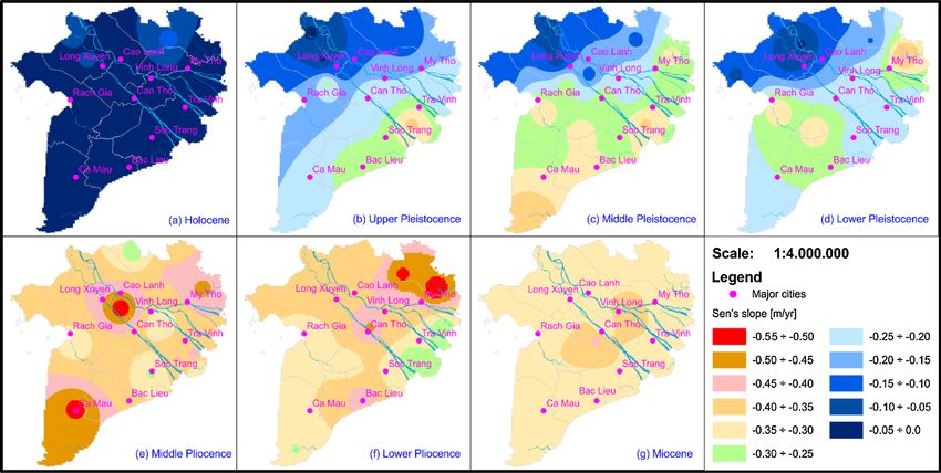
N.L. Duy et al. Journal of Hydrology: Regional Studies 33 (2021) 100746
estimates of groundwater recharge and the response between surface water and alluvial aquifers can be difficult to obtain, and sig
nificant uncertainties exist in groundwater storage in alluvial settings. Under impacts of climate change and human activities (Syvitski
et al., 2009; Vörösmarty et al., 2009; Hirabayashi et al., 2013), which challenge national to global food security (Kummu et al., 2012),
understanding the mechanisms of alluvial aquifers is fundamental.
The Vietnamese Mekong Delta (VMD), an alluvial delta forming the southern tip of Vietnam, is home to 18 million people and plays
a vital role in the country’s food security and economy (Renaud and Kuenzer, 2012). Groundwater resources management is one of the
prerequisites for living and livelihood in the VMD. The extensive hydrological manipulation of the delta has a direct impact on
groundwater resources, mainly through the disruption of natural flood regimes, groundwater exploitation and artificial groundwater
recharge, and salt intrusion in the alluvial aquifers (Renaud and Kuenzer, 2012). Since the 1990s, groundwater has been increasingly
utilized for irrigation, domestic, and industrial purposes (Danh and Khai, 2015), while the extraction has been poorly managed
(Wagner et al., 2012). Unsustainable groundwater abstraction causes declining groundwater levels (Erban et al., 2014) and land
subsidence (Minderhoud et al., 2017) in the delta.
The dynamics of surface water have been continuously highlighted in a number of publications denoting increasing trends in water
level (Dang et al., 2016; Fujihara et al., 2016), sedimentation (Hung et al., 2014b, a; Manh et al., 2015) and floodplain inundation
(Dung et al., 2011; Triet et al., 2017). Analyses on groundwater dynamics are, however, scarce in the VMD. Instead, groundwater
studies have focused on the arsenic contamination of aquifers (e.g., Shinkai et al., 2007; Buschmann et al., 2008; Kocar et al., 2008;
Erban et al., 2013; Huang et al., 2016), groundwater quality (e.g., Wilbers et al., 2014; An et al., 2018; Tran et al., 2019), groundwater
recharge sources (Ho et al., 1991; An et al., 2014), or shallow groundwater transit time (Duy et al., 2019). Notably, these studies mostly
focused on local areas (e.g., provinces or cities) rather than the whole delta. At the larger scale, groundwater has been reported to be
considerably controlled by the river system (Wagner et al., 2012) and closely connected to the surface water in the floodplains (Kazama
et al., 2007). However, information on water flow processes in the multi-layered alluvial aquifer system based on numerical modeling
(e.g., Vermeulen et al., 2013; Shrestha et al., 2016; Hung Van et al., 2019) is scarce due to the complexity of the hydrogeological
subsurface system (Wagner et al., 2012) and the sparsity of groundwater level and lithological data (Johnston and Kummu, 2012). To
our best knowledge, groundwater dynamics focusing on the recent trend of groundwater levels, the “memory effect” (Mangin, 1984;
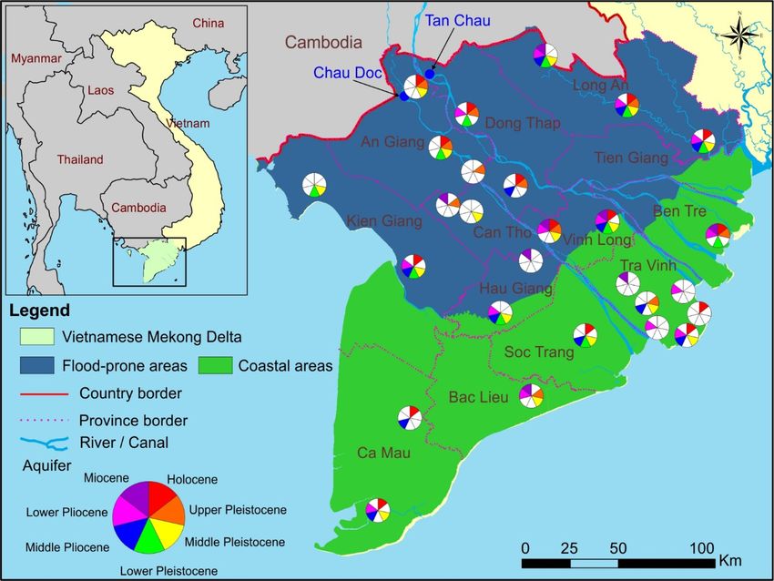
Fig. 1. Study site in the Vietnamese Mekong Delta. The pie charts indicate the location of national stations monitoring groundwater levels within
seven aquifers. Color/white pie segments denote that a monitoring borehole is available/unavailable at a given aquifer, respectively.
2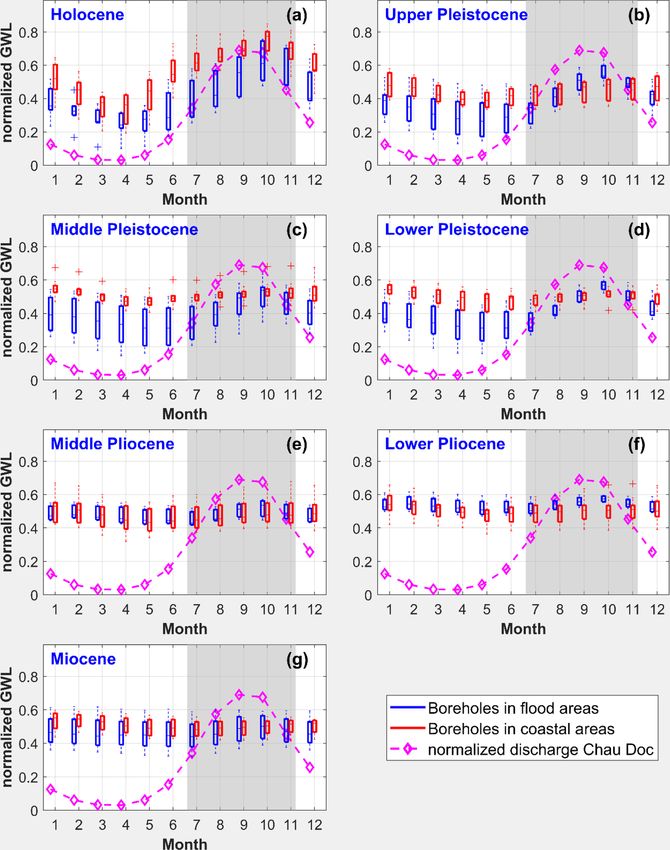
N.L. Duy et al. Journal of Hydrology: Regional Studies 33 (2021) 100746
Massei et al., 2006; Duvert et al., 2015) (representing the time that an aquifer holds water), and the response time between surface
water and alluvial aquifers have not been quantified for the VMD.
Time-series analysis (e.g., Box et al., 2011, 2015), such as trend analysis and correlation analysis, have been frequently applied to
study the dynamics of a groundwater system (Bakker and Schaars, 2019).. Decomposition analysis (e.g., Shamsudduha et al., 2009;
Lafare et al., 2016; Wunsch et al., 2018) and/or predefined response functions (e.g., von Asmuth et al., 2002) can be additional tools to
characterize the hydrologic behavior of a groundwater system. For trend analysis, the nonparametric Mann-Kendall test (Mann, 1945;
Kendall, 1948) and Sen’s slope estimator (Sen, 1968) are commonly applied in hydrological studies (see Madsen et al., 2014 and
references therein). To examine the memory effect and the impulse response of an aquifer, the pioneering work of Mangin (1984)
demonstrates that correlation analysis (auto-correlation and cross-correlation) can be used. Aquifers can act as filters to transform
input signals into output signals by transfer functions (Labat et al., 2000), which can be interpreted to gain insight into the function and
structure of aquifers (Delbart et al., 2014). Following the methodology of Mangin (1984), numerous studies have reported the memory
effect and response of groundwater in karst systems (e.g., Larocque et al., 1998; Massei et al., 2006; Mayaud et al., 2014; Delbart et al.,
2016). In alluvial systems, however, these concepts have found limited application and need further testing (Imagawa et al., 2013;
Duvert et al., 2015).
In this study, groundwater flow processes in the alluvial aquifers of the VMD are investigated by trend and correlation analysis, as
well as time-series decomposition. All these analyses are incorporated into a moving window approach to identify non-stationary
responses. We investigate (1) trends in groundwater levels, (2) the memory effect of alluvial aquifers, and (3) the time-variant
response between surface water and groundwater throughout the VMD. The results are essential for groundwater resource manage
ment and livelihoods in the region, and highlight the general mechanisms of sub-surface water transport in alluvial settings.
2. Study area
The study area is the VMD covering an area of 4 million hectares between 8.5–11.5 ◦ N and 104.5–106.8 ◦ E (Fig. 1). The delta has an
extremely low mean elevation (− 0.8 m above sea level) (Minderhoud et al., 2019). During the flood season (July-November), 35–50 %
of the delta is flooded, mainly by river discharge exceeding bank level. The resulting inundation reaches depths of up to 4.0 m for 3–6
months (Toan, 2014), constituting inundation areas that recharge water to alluvial aquifers. In this study, the inundation areas were
adapted from Triet et al. (2017). These areas cover a territory of approximately 2.0 million hectares in the northern part of the VMD
(Fig. 1). According to Danh and Khai (2015), groundwater in the VMD is typically accessed via private tube-wells (more than 1 million
shallow tube-wells across the delta) at depths of 80− 120 m, and groundwater abstraction wells of water supply plants, reaching depths
of 200− 450 m. The total groundwater abstraction was estimated at approximately 2.5 million m3 per day in 2015 (Minderhoud et al.,
2017).
The multi-layered aquifer system in the VMD has an alluvial basin structure. The deepest area of the basement is located below the
Mekong and Bassac Rivers and rises to the Northeast, North, and Northwest borders (Anderson, 1978; Wagner et al., 2012). Sediments
were deposited during transgression and regression events around 6000–5000 yr BP (Lap Nguyen et al., 2000), resulting in a highly
complex stratigraphy. The subsurface structure and hydrogeological units in the VMD are classified according to geological formations:
Holocene, Pleistocene, Pliocene, and Miocene aquifer systems (Wagner et al., 2012). These aquifers are located below ground level
around 0− 49 m, 31− 193 m, 153− 381 m, and 275− 550 m, respectively (cf. Table 1S in the Supplement). These age units can be
sub-divided into eight hydrogeological aquifer systems: Holocene (qh), Upper Pleistocene (qp3), Middle Pleistocene (qp2–3), Lower
Pleistocene (qp1), Middle Pliocene (n22), Lower Pliocene (n12), Upper Miocene (n31), and Middle Miocene (n2–3 1 ). Generally, each unit
consists of two layers: (i) a low-permeable aquitard layer composed of silt and clay; and (ii) a high-permeable aquifer layer composed
of fine to coarse sand and gravel. The horizontal hydraulic conductivities of the aquitards and aquifers are in the range of (3–40)*10− 8
m/s and (1–20)*10− 4 m/s, respectively. The hydrogeological characterization of these semi-confined aquifers is given in (Wagner
et al., 2012), and their lithological nature and hydraulic properties are described in (Minderhoud et al., 2017) and summarised in
(Hung Van et al., 2019). In this study, the Middle Miocene (n2–3
1 ) was not considered due to a lack of data.
3. Methods
3.1. Datasets
Groundwater levels (GWL) in the VMD have been recorded starting from the mid-1990s at multiple temporal resolutions (from
daily to monthly) and with different monitoring duration (8–22 years). We collected GWL time series between 1996 and 2017 from 88
boreholes (Table S1 in the Supplement) at 27 distributed well nests (Fig. 1). From these data sets the borehole data series with temporal
resolutions higher than weekly and monitoring durations longer than ten years were selected. The datasets were supported by the
project “Research on improvement for the efficiency of water resources monitoring system for early warning of depletion and saline
intrusion in the Mekong Delta plain – No. ĐTĐL.CN-46/18“, which is funded by Ministry of Science and Technology (MOST). An
hourly discharge time series from 1996 to 2017 at Chau Doc was also collected to represent the variability of surface water in the VMD
in the analysis. The discharge data was provided by the Southern Institute of Water Resources Research (SIWRR). For consistency, all
collected data were aggregated to weekly mean values.
3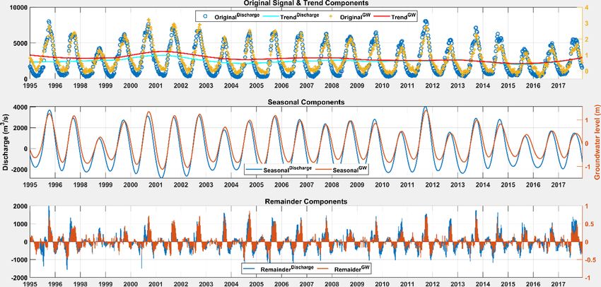
N.L. Duy et al. Journal of Hydrology: Regional Studies 33 (2021) 100746
3.2. Time-series decomposition
We applied a nonparametric time-series decomposition approach known as “STL: Seasonal-Trend decomposition procedure based
on LOESS” (Cleveland et al., 1990). The STL method uses locally weighted regression (LOESS) operations with different moving
window lengths to separate a time series into three distinct components. Eq. 1 shows the additive decomposition of the trend (Tt),
seasonal (St), and remainder (Rt) components from the original signal (Yt).
Yt = Tt + St + Rt (1)
Typically, each component can be related to different processes acting during the generation of the time series. In the case of GWL
time series, the role of each component was classified by (Lafare et al., 2016) as follows:
• Tt represents the long-term processes operating over the period of the entire time series;
• St represents a cyclical process, e.g., the annual cycles resulting from recharge periods;
• Rt represents local processes that cause variability between cycles and can thus be attributed to shorter-term events or impacts (e.g.,
the local recharge and/or abstraction) on the groundwater system.
There is no unique choice for selecting the smoothing parameter (e.g., the length of the moving window) within the STL algorithm.
In many applications, the decision should be based on the goals of the analysis and the knowledge about the mechanisms generating
the time series (Cleveland et al., 1990). While a large value can result in similar components in all years, a small value can track the
observations more closely (Shamsudduha et al., 2009). In this study, we selected a 10-years window for the trend component and
1-year window for the seasonal component. In this way we were able to highlight decadal trends and annual cycles.
3.3. Identification of GWL variability
We calculated the ratio between the variance of decomposed components and the original signal (Eq. 2) to measure the relative
importance of the variance associated with each component in comparison to the original signal. Graphical comparison of these ratios
(Lafare et al., 2016) and the boxplot of seasonal variation of normalized time series were used to characterize the relative variability of
GWL in the VMD.
RatioTrend = Variance(Tt)/Variance(Yt) (2a)
RatioSeasonal = Variance(St)/Variance(Yt) (2b)
Ratio Remainder
= Variance(Rt)/Variance(Yt) (2c)
3.4. Trend analysis
We applied the Mann–Kendall (MK) nonparametric trend test (Mann, 1945; Kendall, 1948) with Sen’s slope (Sen, 1968) to
investigate recent changes (1996–2017) of the groundwater system in the VMD. The trend magnitude was reported as Sen’s slope
considering a significance level of 95 %. Trends were calculated by a moving-window approach (10-year window with 1-year
increment of the original groundwater level time series) to investigate the time-variations of trends. Spatial patterns of Sen’s slope
were mapped at the regional scale using GIS built-in interpolation models and geostatistical Kriging techniques in ArcGIS version 10.4.
Time-series were analyzed using MATLAB R2019b with the Statistics Toolbox version 11.6.
3.5. Auto-correlation
Auto-correlation analysis was used to identify the memory effect (Mangin, 1984; Massei et al., 2006; Duvert et al., 2015) of alluvial
aquifers in the VMD. We applied the auto-correlation to the remainder component (Rt), because it represents the local effects and
short-term events (Lafare et al., 2016), while the trend and seasonal components are by definition significantly auto-correlated. The
auto-correlation of a time-series x is defined as (Box et al., 2015):
∑ k
N − 1 N−
i=1 (xi − x)(xi+k − x)
rx (k) = (3)
2σx
Where rx (k) is the autocorrelation coefficient at lag k, and x is the arithmetic mean of the time series with N observations. σx is the
standard deviation of the time series. The value of k was selected smaller than the cutting point (N/3) to avoid stability problems. The
memory effect of the signal was defined as the time lag when rx (k) reached a value of 0.2, as frequently applied in GWL studies
(Mangin, 1984). The value was termed as the de-correlation time lag (k0.2) here. Alternatively, the memory effect was also charac
terized by the overall shape and magnitude of the auto-correlogram (Massei et al., 2006). We quantified the slope of the
auto-correlogram by logarithmic fits, following (Massei et al., 2006; Duvert et al., 2015):
4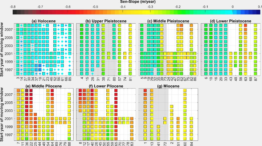
N.L. Duy et al. Journal of Hydrology: Regional Studies 33 (2021) 100746
rx (k) = αlog(k) + β (4)
where α (week− 1) and β (dimensionless) are slope and intercept of the logarithmic function, respectively. Typically, α describes the rate
at which the correlation decreases during the study period, and β corresponds to the loss of correlation for a unit lag k.
3.6. Cross-correlation
Cross-correlation, represented by a cross-correlogram, identifies the relationship between two signals. The cross-correlation be
tween two time series x and y with N observations is defined as (Box et al., 2015):
∑ k
N − 1 N−
i=1 (xi − x)(yi+k − y)
Rxy (k) = (5)
σx σy
Where Rxy (k) is the cross-correlation coefficient at lag time k, x and y are the arithmetic means of the two time series and σ x and σy are
the standard deviations.
The cross-correlation analysis was applied in a moving-window approach (1-year window with 1-week increment) to highlight the
inter-annual variability of the response time of groundwater levels to changes in discharge. For each window, the cross-correlogram
function between input and output was calculated, and the response time τ (the lag time k corresponding to the maximum correlation)
was identified, following Delbart et al. (2014) and Duvert et al. (2015). Only a cross-correlation coefficient higher than the standard
error of 2/N0.5 (corresponding to 95 % confidence level) was accepted. N is the number of observations in the moving window (Diggle,
1990). Readers are referred to Delbart et al. (2014) for a graphical example of the sliding cross-correlation method.
The response time evaluated by the cross-correlation analysis alone can be less accurate if the autocorrelation of the input signal is
high (e.g., close to 1) (Bailly-Comte et al., 2011). In order to reduce this effect, the autocorrelation of the input can be removed by
prefiltering the input signal (e.g., removing all serial dependencies such as trend, seasonal, and autoregressive components). By this
pre-whitening procedure, white noise residuals are obtained (Watts and Jenkins, 1968). The analyses of time-series decomposition
undertaken in this study (see section 3.2) can be considered as an appropriate approach to prefilter the input signal. Therefore, we used
the remainder component of river discharge (at Chau Doc) as an input signal in the cross-correlation analysis. We assumed that the
selected input signal represents random, un-correlated processes in surface water (e.g., unaffected by the trend, seasonal, and
autoregressive components). The output signal was the remainder component of the GWL time-series. It is noted that groundwater
recharge in the VMD is considered to stem mainly from surface water (Wagner et al., 2012). We assumed that the precipitation ponding
on the ground is mixed with preexisting surface water (e.g., river water and/or floodwater) before infiltrating to the groundwater. This
means that all types of recharge sources were summed up in the “surface water” component. In this context, the time-series of τ gives
information about the impulse response that transfers surface water into the aquifers of the VMD.
Fig. 2. STL decomposition of weekly discharge (at Chau Doc) and GWL time series (borehole No. 14). Trends Tt (top), seasonal components St
(middle) and remainder components Rt (bottom). Left and right axes denote for discharge (m3/s) and groundwater level (m), respectively.
5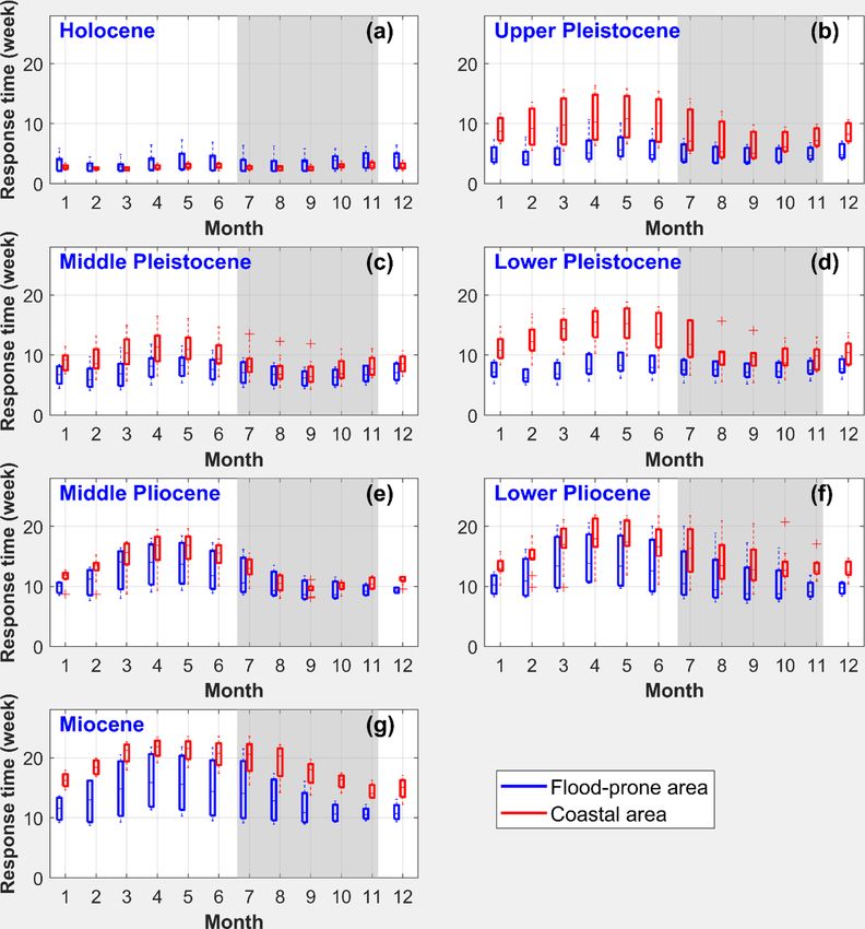
N.L. Duy et al. Journal of Hydrology: Regional Studies 33 (2021) 100746
4. Results
4.1. Variability of GWL time series
Fig. 2 shows an example of the decomposition of weekly discharge (at Chau Doc) and the GWL time series (at borehole No. 14)
using the STL algorithm. The plot highlights both seasonality and long-term trends in GWLs. The results of the time-series decom
position analysis showed that the relative magnitude of each component varies considerably across the delta. Therefore, the relative
variability of the GWL was assessed based on the variances of the trend, seasonal, and remainder components along with the variance
of the original time series. This relative variability (represented by the variance ratios defined by Eq. 2) is plotted in Fig. 3.
The decomposition of the time-series revealed a higher variability of the seasonal component in the shallow aquifers (e.g., Ho
locene), and the dominant variability of the trend component in the deep aquifers (e.g., Pliocene and Miocene). For example, the trend
component represented more than 90 % and less than 55 % of the variance of the original time series for deep and shallow aquifers,
respectively (Fig. 3). For the Pleistocene aquifer, the GWL time series were separated into two distinct clusters dominated by the
seasonal (cluster 1) and trend components (cluster 2) in Fig. 3. However, there was no apparent relationship between the borehole
depth and the variance of components in the Pleistocene aquifers, as indicated by the wide scatter without any grouping of the
“Pleistocene” symbols in Fig. 3.
To highlight the seasonal variation, each time-series was normalized to values between 0 and 1 by subtracting the minimum value
and dividing by the total range. Fig. 4 is a boxplot of the normalized time series of GWLs and river discharge. Higher GWLs were
observed in the flood season. The amplitude of the seasonal variation of GWLs decreased with increasing borehole depth, from sub
stantial seasonal variation in the Holocene aquifer to no seasonal variation in the Pliocene and Miocene aquifers. Comparing between
flood and coastal areas for shallow groundwater, a similar seasonal pattern was observed for the Holocene aquifer. In contrast, the
GWLs in flood-prone areas varied slightly more than those in coastal areas for the Pleistocene aquifers.
4.2. Trend of groundwater levels
Fig. 5 shows the results for recent (1996–2017) trends of GWLs across the VMD. The GWL in all aquifers showed various magnitudes
of decreasing trends from 0.01− 0.55 m/year (all significant at the 95 % level). The strongest negative trends were observed mainly in
areas around major cities and major industrial areas (e.g., Tan An, Cao Lanh, Long Xuyen, Can Tho, and Ca Mau). Moreover, stronger
declining trends were detected in deeper aquifers with the highest decrease (0.30− 0.55 m/year) in the Pliocene and Miocene aquifers.
The weakest declining trends (0.01− 0.11 m/year) were observed in the Holocene aquifer. The medium depth Pleistocene aquifers
showed decreasing trends in-between the trends of the deep and shallow aquifers, with values of 0.05− 0.28 m/year and 0.22− 0.41 m/
year for boreholes located at flood and coastal areas, respectively. An increasing trend was not found for any of the investigated
boreholes.
A comprehensive analysis of the time-variant trends (10-year periods with 1-year increments) is presented in Fig. 6. Similar to the
previous analysis, we observed declining trends in GWLs at all aquifers with higher magnitudes in deeper aquifers. However, no
significant trends were detected for some short-term periods for the Holocene aquifer. For other aquifers (e.g., Pleistocene, Pliocene,
and Miocene), all declining trend patterns are significant at the 95 % level. Except for the Holocene aquifer, the magnitude of the
declining trend for almost all boreholes was considerably higher in later periods (e.g., after 2007) than in early periods. For example,
Fig. 3. Variability ratios (defined by Eq. 2) associated with each time series component for the different aquifers. The color bar indicates the depth
of the borehole (m).
6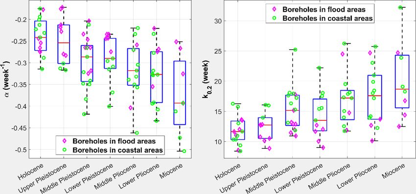
N.L. Duy et al.                                                                                 Journal of Hydrology: Regional Studies 33 (2021) 100746

Fig. 4. Seasonal variation of normalized GWL and discharge at Chau Doc station. The box-whisker plots show the interquartile ranges; the whiskers
show the minimum and maximum values associated with 1.5 times the interquartile range. The grey areas mark the monsoon/flood season.

the declining trend before 2006 was around 0.1− 0.35 m/year but increased up to 0.6− 0.75 m/year after 2007 (Fig. 6). Hence, the
decrease of GWL accelerated over the last two decades. The strongest declining time-variant trends were observed in the Pliocene
aquifer, particularly close to big cities such as Ca Mau (borehole No. 22), Can Tho (borehole No. 40), Dong Thap (borehole No. 36), and
Long An (borehole No. 65). In line with the overall trends (Fig. 5), the GWLs in coastal areas decreased more strongly than in flood-

                                                                       7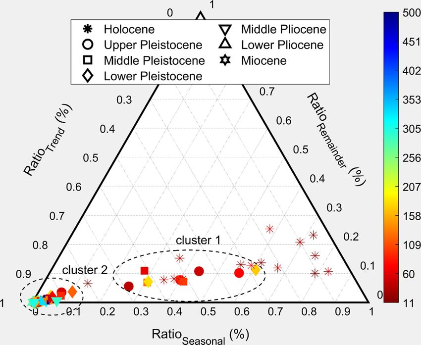
N.L. Duy et al.                                                                                     Journal of Hydrology: Regional Studies 33 (2021) 100746

                      Fig. 5. Spatially interpolated recent (1996–2017) trends of GWLs of the different aquifers in the VMD.

Fig. 6. Time-variant trends (reported as Sen’s slope) calculated for ten-year periods in different aquifers in the VMD. The y-axis shows the start year
of the moving window, while the x-axis shows the borehole number (Table S1). The values of Sen’s slope (m/year) correspond to the color bar. The
squares and circles indicate that the trends are significant or insignificant at the 95 % level, respectively. Grey (or white) backgrounds indicate that
the location of a borehole is at flood-prone (or coastal) areas. Blank areas indicate no available GWL data.

                                                                           8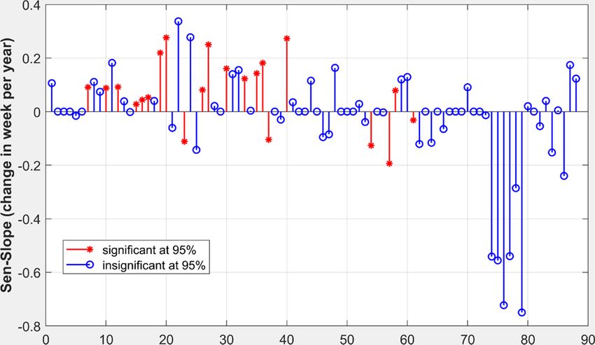
N.L. Duy et al.                                                                                     Journal of Hydrology: Regional Studies 33 (2021) 100746

prone areas for the Pleistocene aquifers. For the Holocene and Miocene aquifers, the magnitude of the declining GWL trends was not
significantly different between flood-prone and coastal areas.

4.3. Memory effect of alluvial aquifers

    From the remainder component of each GWL time series, an auto-correlation function was derived. Distinct behaviors were
observed among the 88 auto-correlograms, with various degrees of groundwater memory effect. Fig. 7 shows the rate of decrease of the
auto-correlation function (α), together with the de-correlation time lag (k0.2) when the auto-correlation coefficient (rx ) of 0.2 was
reached. Both methods (logarithmic fit and de-correlation time lag) highlighted similar results. Typically, a stronger memory effect
was detected for deeper aquifers, as depicted by more negative α and higher k0.2 (Fig. 7). Stronger memory effects were also identified
for boreholes located in coastal areas compared to those in flood-prone areas; this behavior was, however, not apparent for Holocene
aquifers. The de-correlation time lag of the Holocene aquifer was between 5 and 17 weeks. The time lag of the Pleistocene aquifer was
between 6 and 26 weeks, showing two distinct groups of flood-prone and coastal areas. The range of the time lag of Pliocene and
Miocene aquifers was 11–27 weeks and 13–33 weeks, respectively.

4.4. Response time analysis

    The moving-window cross-correlation analysis was performed between the remainder component of discharge at Chau Doc
gauging station and of GWLs at 88 boreholes. Depending on the length of each GWL time series, 523 to 1098 moving windows were
obtained applying a window length of one year and moving in one-week increments. For example, a borehole with 10-year monitoring
GWL will result in a sequence of 523 one-year moving windows. Consequently, we obtained 88 time-series of response time τ with
different time lengths (e.g., 523− 1,098 values per time series of τ depending on the number of moving windows detected for each
borehole). Each time series of τ was then averaged by calculating the arithmetic means of the τ values falling in the month of the year.
This analysis is meant to highlight seasonal differences in water level response. It is noted that the shape of the cross-correlogram
varied considerably between boreholes. Only cross-correlation coefficients higher than the standard error of 0.28 (corresponding to
the 95 % confidence level) were accepted. The variability of the response time was reported for every month in Fig. 8, showing the
seasonal variation of the time required for the pulse of surface water to reach the alluvial aquifers.
    Generally, we observed high variability in response time in the alluvial multi-aquifer system. Shorter response time was observed
for shallow groundwater compared to deep groundwater (Fig. 8). The response time range increased from the Holocene (1.9–7.3
weeks) to the Pleistocene (3.7–18.9 weeks), the Pliocene (7.5–22.5 weeks), and the Miocene aquifers (9.1–23.8 weeks). Except for the
Holocene aquifer, apparent seasonal variation of response time was observed for all aquifers, and the response times in the flood-prone
areas were shorter compared to those in the coastal areas. The variability of response time in both flood and dry seasons for the
Holocene aquifer was insignificant. For other aquifers, response time varied seasonally, with lower values during the flood season. The
shortest response time was detected mainly in the peak flood period (e.g., September or October), with the longest response time at the
end of the dry season (e.g., May). Most likely this was caused by the higher hydraulic head in the surface water during the flood season.
Notably, due to a low number of monitoring boreholes in the Pliocene and Miocene aquifers (3–4 boreholes in each aquifer, cf. Fig. 7),
the identification of response-time variations in these aquifers in the flood-prone areas might be impaired.
    Long-term changes of the response time within the individual boreholes were analysed by the Mann–Kendall nonparametric trend

Fig. 7. Memory effect of aquifers in the VMD, characterized by (α) the rate of decrease of the autocorrelation function (left), and (k0.2) the lag time
(week) to reach the autocorrelation coefficient of 0.2 (right).

                                                                          9
N.L. Duy et al.                                                                                 Journal of Hydrology: Regional Studies 33 (2021) 100746

Fig. 8. Response time, averaged for each month, between surface water and groundwater for different aquifers in both flood-prone and coastal areas
in the VMD. Grey areas indicate flood season.

test, applied on the moving time windows. Results of Sen’s slope (considering a significance level of 95 %) are reported for 88
boreholes in Fig. 9. Long-term changes in response time were found to be negligible. Only 20 boreholes showed minor significant
changes in Sen’s slope of less than 0.3 weeks per year. No significant long-term change was observed for all other wells.

5. Discussion

5.1. Potential of groundwater recharge and role of alluvial aquifers in the VMD

   The decreasing magnitude of seasonal variation from shallow to deep groundwater (Fig. 4) suggests that the alluvial aquifers act as
low-pass filters during the transformation of input signals (e.g., river discharge or water levels) into output signals (e.g., groundwater
water levels), resulting in increasing memory effects (Fig. 7) and response times (Fig. 8) with aquifer depth in the VMD. The role of
aquifers as a low-pass filter in the frequency domain has also been reported in other alluvial settings (e.g., Imagawa et al., 2013; Duvert

                                                                       10
N.L. Duy et al. Journal of Hydrology: Regional Studies 33 (2021) 100746
Fig. 9. Long-term changes of the response times (reported as Sen’s slope in the y-axis) relative to the monthly mean response time for the 88
boreholes (x-axis) in the VMD.
et al., 2015).
Regarding shallow aquifers, the dominance of the seasonal variability (Fig. 3) and similar patterns of seasonal fluctuations between
GWLs and surface water (Fig. 4) suggest a good hydraulic connection between river water and shallow aquifers (i.e. Holocene and
Pleistocene) across the delta. This result is in line with the findings of Wagner et al. (2012) that shallow groundwater is effectively
connected to surface water (e.g., rivers, irrigation channels, or floodplains) in the area. This connectivity, as expressed by higher
seasonal variabilities (Fig. 4b, c, d), is more pronounced in the flood-prone areas compared to the coastal areas. Such effective
connection suggests a high potential for groundwater recharge from surface water to shallow aquifers, particularly for locations in the
flood-prone areas, where long-lasting and widespread inundations occur regularly. The inundations create a strong hydraulic head
differences and provide sufficient water volume for shallow GW recharge, which is missing in the coastal region. Therefore the sea
sonal signal observed in the coastal shallow aquifers has to be attributed to different sources or causes. The most plausible source is
likely the lateral inflow of waters that originate from the upstream region, i.e. inundated areas, as suggested by Hoang and Bäumle
(2019). During the flood season, the hydraulic head in the shallow aquifers underneath the inundated areas rises and creates a head
difference for lateral downstream flow within the aquifers towards the coastal region. The seasonal signal is thus dampened because of
the flow time, distance and available volume. This seasonal component is additionally dampened in the coastal region by the relatively
constant head caused by the ocean.
For deep groundwater, low permeable aquicludes appear to limit the recharge to the deeper aquifers (Pliocene and Miocene
aquifers) both in flood-prone and coastal areas. The dominance of trend components (Fig. 3) and the low variation of GWLs in the
Pliocene and Miocene aquifers (Fig. 4e,f,g) corroborate these findings. Significant increasing memory effect and response time with
depth (Fig. 7 and Fig. 8) also indicate that the recent recharge to deep aquifers, if any, is very limited. Hence the deeper aquifers may be
hardly replenished by surface water sources including precipitation sources in the VMD. Hung Van et al. (2019) pointed out that the
freshwater from the upper system cannot infiltrate deeper than about 350 m. Considering our results and the literature, any potential
recharge of the deeper aquifers is very unlikely to originate from vertical infiltration through the aquiclude layers, but rather from the
lateral flow within the aquifers from upstream areas. The deeper aquifers are located closer to the surface in the highland areas of
southern Vietnam (e.g. Binh Phuoc) or Cambodia (Ha et al., 2019). The presented analysis implies that the vertical recharge pathway
via aquiclude layers and inter-aquifer connectivity in the multi-aquifer system is insignificant in the VMD. This, in turn, means that a
natural replenishment of the over-exploited deeper aquifers as the primary freshwater sources in the VMD cannot be achieved locally
by natural pathways. Instead, recharge could depend on the infiltration processes and management and exploitation of the deeper
aquifers in the neighboring regions, particularly Cambodia. This also means that recovery of GW levels in the deeper aquifers requires a
substantial amount of time.
Additionally, the operation of all planned dams in the Mekong basin will most likely reduce flood season flow. A potential
consequence of this is the reduction of recharge to the aquifers in the VMD, both the shallow aquifers (recharge within the VMD) and
deeper aquifers (recharge from the inundated areas in the Cambodian part of the delta). This finding is in line with Kazama et al.
(2007), who stated that a 44 % reduction in flooding areas could result in a 42 % decline of shallow groundwater storage in the Mekong
delta. Weighing the potential impacts of climate change and reservoir operation on the Mekong hydrology on groundwater recharge,
the negative impacts of reservoir operation will more likely overwrite the possible positive effects of increased flood season flow under
climate change projections (Lauri et al., 2012). Although a quantitative assessment of the effects of dam development on groundwater
recharge has not been carried yet, the presented results imply that any substantial negative changes in flood volume and floodplain
inundation could impair the recharge of groundwater in all aquifers in the VMD. This aspect should be considered in long term
strategic planning of the management of the groundwater resources, in addition to the urgently needed short-term limitation of current
GW exploitation.
11N.L. Duy et al. Journal of Hydrology: Regional Studies 33 (2021) 100746
5.2. Drivers of GWL declines
Extending the findings of previous studies (e.g., Wagner et al., 2012; Erban et al., 2014), this work uses more recent data to confirm
the previously observed decrease of GWLs in deeper aquifers in the VMD by time-variant trend analysis based on high-frequency
groundwater observations considering both shallow and deep aquifers. The overall variabilities of the declining trends of GWLs
confirm the decrease rate of 9− 78 cm/year reported in Erban et al. (2014), i.e. indicate that GW over-exploitation continued in the last
decade. Our results indicate that groundwater abstractions highly exceeded groundwater recharge, resulting in a considerable
decrease of GWLs and groundwater storage in the VMD over the last 22 years.
The lesser changes in GWL in the shallow aquifers, however, are a result of the interplay between the good connectivity to and
recharge from surface water, the compaction of the young sediment composing the aquifers (Wagner et al., 2012), and the compar
atively low abstraction from these shallow aquifers. These factors compensate each other, resulting in the observed overall low decline
in the shallow aquifers. On the contrary, the significant decrease of GWLs in the deeper aquifers can be linked to the lower recharge
rates (section 5.1) and to the high amount of groundwater abstraction. Groundwater in the Pliocene and Miocene aquifers has good
drinking water quality and is thus heavily used. The highest decreasing trends were identified mainly for urban areas with high
population densities (Fig. 5), and thus indicate that human activities are very likely the dominant driver of this GWL decline. Moreover,
in coastal regions saltwater intrusion in surface water impedes the use of shallow groundwater as a drinking water source or for
irrigation (cf. Fig. 2 Smajgl et al., 2015). Therefore groundwater is the key source of freshwater for domestic uses and agricultural
production in the coastal regions (Wagner et al., 2012). The pronounced decreasing trend of GWLs in the coastal areas compared to the
flood-prone areas in the Pleistocene aquifers (Fig. 5b, c, d) thus provides evidence for a significant and non-sustainable groundwater
abstraction in the coastal areas. For example, groundwater is highly exploited for domestic freshwater supply in Ca Mau peninsula. The
results presented in this study indicate that the high demands for groundwater resources cannot be compensated by the limited
recharge. According to Danh and Khai (2015), groundwater in the VMD is typically accessed via private tube-wells (more than one
million over the whole delta) at depths of 80− 120 m (corresponding to Pleistocene aquifers), and abstraction wells of freshwater
supply plants, reaching depths of 200− 450 m (corresponding to the Pliocene and Miocene aquifers). Therefore the decline of GWLs in
the Pleistocene aquifers can be attributed to household demand. In contrast, the decrease in the Pliocene or Miocene aquifers can be
linked to the demand of water supply plants, and thus the general water demand of the population and economy.
The acceleration of the decrease of GWLs (Fig. 6) can be linked to the increasing trend in groundwater exploitation, and the
consequent widespread land subsidence for the VMD (Erban et al., 2013, 2014; Minderhoud et al., 2017), similar to many deltas and
coastal areas around the world (see Gambolati and Teatini, 2015). Our study suggests that the current groundwater exploitation
already exceeds aquifer recharge capacities in the VMD. Due to the demand for socio-economic and industrial development,
groundwater exploitation is forecasted to further increase in the future (Danh and Khai, 2015). A further severe decline of GWLs would,
however, accelerate saltwater intrusion into the alluvial aquifers, groundwater contamination, land subsidence, and thus threaten
sustainable development in the entire delta (Minderhoud et al., 2017).
5.3. Groundwater memory effect in alluvial settings
The analysis of the auto-correlation with the logarithmic fits and the de-correlation time provides insights into the memory effects
in the different aquifers. For shallow groundwater, the short memory effect indicates a good hydraulic connection to surface water, and
thus a high potential for groundwater recharge. This was to be expected from the geological setting. Following the same logic, long
memory effects in the deeper aquifers, indicate a poor hydraulic connection to surface water and thus limited groundwater recharge.
Because groundwater storage can be attributed to structural factors that are difficult to assess (e.g., the change in grain size of the
aquifer material or its degree of compaction, which can change the hydraulic conductivities and groundwater outflow) (Duvert et al.,
2015), the presented analysis of the memory effects might serve as a proxy-information on potential groundwater storage. In the VMD,
the memory effect of alluvial aquifers varies according to the geographical location (Fig. 7). Groundwater memory increases in both
vertical and horizontal directions: (1) from shallow to deep aquifers, and (2) from upstream (i.e., flood-prone regions) to downstream
(i.e., coastal areas). The vertical increase of the memory effect from shallow to deep aquifers can be attributed to the existence of
low-permeable aquicludes between aquifers. The aquicludes between deep aquifers (Pliocene and Miocene) are thicker and charac
terized by lower hydraulic conductivities compared to the shallow aquifers (Holocene and Pleistocene) (Hung Van et al., 2019). These
aquicludes act thus as low-pass filters in the frequency domain weakening the variation of GWLs at the deep groundwater in the VMD.
This behavior was also reported for similar geological settings, e.g. for alluvial aquifers in the Shiga Prefecture, Japan (Imagawa et al.,
2013) and southeast Queensland, Australia (Duvert et al., 2015). Similarly, the horizontal spatial differences of the memory effect may
be caused by the spatial variation of physical properties (e.g., hydraulic conductivity and thickness) of the aquifers (Zhang and
Schilling, 2004). In this context, an explanation for the generally higher memory effect from upstream to downstream in the VMD
could be the higher thickness of the aquicludes in coastal areas compared to flood-prone areas, as per Fig. 2 in Hung Van et al. (2019).
Generally, longer memory effects indicate higher water storage capacities, particularly in the case of the deep alluvial aquifers in
the VMD. A similar explanation for longer memory effects and groundwater storage was given by Mangin (1984) and Imagawa et al.
(2013). This means that the potential for groundwater storage and restoration is higher in the deeper aquifers. This comes, however, at
the cost of longer natural recharge times, which has to be considered in any sustainable GW management plan.
12N.L. Duy et al. Journal of Hydrology: Regional Studies 33 (2021) 100746
5.4. Factors controlling the impulse response between surface water and alluvial aquifers
The moving window cross-correlation analysis shows that the interaction between surface water and groundwater is highly dy
namic and exhibiting strong seasonality. The differences in impulse response between the river and the different alluvial aquifers can
be attributed to (1) groundwater depth, (2) seasonal variability, (3) location (i.e., flood-prone or coastal areas), and (4) existence of
aquicludes. Shorter response times were detected for shallow groundwater, the flood season, and flood-prone regions (Fig. 8). Except
for the Holocene aquifer, the response time of boreholes in flood-prone areas in the dry season are still shorter than those in coastal are
in flood season, indicating that the response time is more controlled by location than seasonal variability. This result supports the
assumption that the deeper aquifers might be recharged from upstream areas of the VMD (see Section 5.1). During the flood season
(July-November), inundation is up to 4.0 m high and lasts for 3–6 months in flood-prone areas (Toan, 2014). River water levels,
inundation depths and soil saturation are higher during the flood period; thus the pressure pulse is transmitted more rapidly and
directly to aquifers compared to the dry period, and sufficient amounts of water (ponding water on inundated floodplains) are
available to recharge the GW. This means in return that a shortening of the flood season very likely reduces groundwater recharge,
because of the associated reduction of high water levels and pressure heads in the rivers, as well as because of the reduction of the
floodplain inundation extent and depths. A shortening of the flood season typically occurs during strong El Niño events (Ruiz-Barradas
and Nigam, 2018), and is also expected as a consequence of the operation of existing and construction of planned dams in the Mekong
basin (Lauri et al., 2012). Due to the long response times, it has to be expected, that this effect will be more pronounced in the deeper
aquifers (Lower Pliocene and Miocene), where the response times are in the range of the duration of the flood season. However, as
climate change scenarios predict an intensification of the Southeast Asian monsoon and an increase in flood season discharge (Hoang
et al., 2016), there are also chances of increasing average recharge of the deeper aquifers in the VMD in the future, provided that the
reservoir operation does not diminish this effect.
5.5. Limitations and wider implications
The time series analysis we are applying is in principle a black-box model, and can only determine mathematical relations (cor
relations) between time series, not causal relationships (Bakker and Schaars, 2019). The approach is thus only suitable to highlight and
visualize the behavior of a groundwater system without an explicit analysis of the underlying physics and/or drivers of system
behavior. Therefore, this study should be considered as the first step towards a characterization of the previously unstudied behaviors
of alluvial aquifers in the VMD. Future research should aim at a quantitative investigation of the drivers of the memory effect and
response time in the VMD. To understand the physical processes of a groundwater system, a physical-based or at least conceptual
groundwater model is required, which is out of the scope of this study.
In this study, time series analysis can provide valuable information about time-variant trends of GWLs, the memory effect, and the
response time for the whole VMD. The visualization of these groundwater dynamics provides an overview on how long an aquifer
stores water (memory effect), how fast an aquifer responds to variations in surface water (response time), and the recently accelerating
decline of GWLs in the VMD. These findings should be considered as initial contributions to the hydrogeological literature of a little-
known groundwater system in alluvial settings. Due to simplicity and ease of interpretation, the applied time series analysis can be an
additional tool, for example, to process data and quickly provide efficient alternatives to calibrate groundwater models (Bakker and
Schaars, 2019). Also, our approach has direct implications for the initial investigations of an understudied groundwater system where
data and/or resources (e.g., human or financial) are insufficient to develop a dynamic groundwater model.
6. Conclusions
This study provides hydrogeological storage characteristics of the alluvial aquifers in the VMD. We examined the groundwater
dynamics focusing on (1) the recent trend of groundwater levels in order to indicate GW over-exploitation, (2) the memory effect of
alluvial aquifers for an assessment of the GW storage, and (3) the response time between surface water and groundwater as a proxy for
GW recharge. GWL time series between 1996 and 2017 from 88 boreholes at 27 national stations were collected, selecting time series
with a sampling resolution higher than once per week and monitoring periods longer than ten years.
The time-series decomposition of GWLs highlights the large seasonal variability in the shallow aquifers and the dominance of the
trend component in the deep aquifers. This indicates an effective connection between the shallow Holocene aquifer and surface water,
and a high potential for shallow groundwater recharge. The low permeable aquicludes separating the aquifers behave as low-pass
filters that reduce the high-frequency signals in the GWL variations, and limit the recharge to the deeper aquifers.
The trend analysis indicates that both shallow and deep aquifers are currently over-exploited and not fully recharged, resulting in a
considerable decrease of GWLs (0.01− 0.55 m/year) and groundwater storage over the last 22 years. Significant downward trends were
detected in the deep aquifers, which is the primary source of GW used for drinking water purposes, compared to weak declining trends
in shallow aquifers, which has a higher potential for groundwater recharge and is much less exploited due to water quality issues. This
study leads to the conclusion that the groundwater abstraction has accelerated the GWL declines. These findings are evidenced by a
stronger declining time-variant trend observed for almost all boreholes in later periods (i.e., after 2007) compared to early periods (i.e.,
before 2006). While the slight decline of GWLs in the Holocene aquifer (0.01− 0.11 m/year) is likely caused by natural variations and
effects (e.g., the compaction of the delta), the significantly declining GWLs of the Pliocene and Miocene aquifers (0.25− 0.55 m/year)
can be attributed to the groundwater over-exploitation particularly around urban and industrial areas in the VMD.
The groundwater memory varies according to the geographical location, being shorter from shallow to deep aquifers, and from
13N.L. Duy et al. Journal of Hydrology: Regional Studies 33 (2021) 100746
flood to coastal areas. The memory effects of shallow and deep groundwater are in the range of 5–17 weeks and 10–33 weeks,
respectively. Interpreting longer memory as higher storage, it can be concluded that the deeper aquifers have a higher storage capacity
than the shallow aquifers.
The moving cross-correlation analysis highlights the highly dynamic interaction between surface water and groundwater. The
response time between the river and alluvial aquifers depends on groundwater depth, seasonal variability, and location. Shorter
response times were detected in the flood season compared to the dry season. The seasonal variability of response time was influenced
by the flood period and the flood timing. Higher water levels during the flood season likely transmit the pressure pulse more rapidly
and directly. Moreover, the response times of the deeper and heavily used aquifers are in the range of the duration of the flood season.
This finding is relevant for any estimation of the recharge to the most important aquifer (i.e., the Pliocene aquifer) of the VMD during
the flood season. It essentially means that this aquifer most likely receives hardly any recharge during shortened flood seasons (like, e.
g., during the frequently occurring El Niño events).
More generally, our study illustrates the usefulness of time-series techniques to understand the mechanisms of groundwater
recharge, discharge and storage in alluvial settings. The findings on the variabilities of GWL trends, the memory effect of alluvial
aquifers, and the response time between surface water and groundwater are primarily highlighted for the VMD. The information is
crucial for groundwater resource management in the VMD. Due to its simplicity, the applied time-series analysis can be easily
reproduced to provide insights on groundwater behavior in other alluvial settings.
Data availability statement
The hydrological data used in this paper are not publicly accessible; however, the authors can be contacted by email to acquire the
data.
CRediT authorship contribution statement
Nguyen Le Duy: Conceptualization, Methodology, Resources, Software, Visualization, Writing - original draft. Triet Van Khanh
Nguyen: Resources, Visualization. Dung Viet Nguyen: Conceptualization, Methodology, Software. Anh Tuan Tran: Visualization.
Ha Thi Nguyen: Resources. Ingo Heidbüchel: Writing - original draft. Bruno Merz: Writing - original draft. Heiko Apel: Writing -
original draft.
Declaration of Competing Interest
The authors declare no competing interests that could influence the work reported in this paper.
Acknowledgements
We want to thank the Southern Institute of Water Resources Research for providing the observed discharge at Tan Chau and Chau
Doc, and the National Center for Water Resources Planning and Investigation for sharing their groundwater database of the Mekong
Delta. N.L.D., N.V.K.T., and T.T.A. received funding from the German Academic Exchange Service (DAAD) and the Catch-Mekong
project (https://catchmekong.eoc.dlr.de/). N.T.H. is chief of the project No. ĐTĐL.CN-46/18 funded by MOST. This work is also
embedded in the Catch-Mekong project (Project No. 02WM1338C by BMBF and KHCN-TNB.DT/14-19/C11 by MOST) and Project No.
ĐTĐL.CN-46/18 by MOST.
Appendix A. Supplementary data
Supplementary material related to this article can be found, in the online version, at doi:https://doi.org/10.1016/j.ejrh.2020.
100746.
References
An, T.D., Tsujimura, M., Le Phu, V., Kawachi, A., Ha, D.T., 2014. Chemical characteristics of surface water and groundwater in coastal watershed, Mekong Delta,
Vietnam. Procedia Environ. Sci. 20, 712–721.
An, T.D., Tsujimura, M., Phu, V.L., Ha, D.T., Hai, N.V., 2018. Isotopic and Hydrogeochemical Signatures in Evaluating Groundwater Quality in the Coastal Area of the
Mekong Delta, Vietnam. Advances and Applications in Geospatial Technology and Earth Resources. Springer International Publishing, Cham, pp. 293–314.
Anderson, H.R., 1978. Hydrogeologic Reconnaissance of the Mekong Delta in South Vietnam and Cambodia, p. 1608R. https://doi.org/10.3133/wsp1608R.
Bailly-Comte, V., Martin, J.B., Screaton, E., 2011. Time variant cross correlation to assess residence time of water and implication for hydraulics of a sink-rise karst
system. Water Resour. Res. 47 (5).
Bakker, M., Schaars, F., 2019. Solving groundwater flow problems with time series analysis: you May not even need another model. Groundwater 57 (6), 826–833.
https://doi.org/10.1111/gwat.12927.
Box, G.E., Jenkins, G.M., Reinsel, G.C., 2011. Time Series Analysis: Forecasting and Control, 734. John Wiley & Sons.
Box, G.E., Jenkins, G.M., Reinsel, G.C., Ljung, G.M., 2015. Time Series Analysis: Forecasting and Control. John Wiley & Sons.
14N.L. Duy et al. Journal of Hydrology: Regional Studies 33 (2021) 100746
Buschmann, J., et al., 2008. Contamination of drinking water resources in the Mekong delta floodplains: arsenic and other trace metals pose serious health risks to
population. Environ. Int. 34 (6), 756–764. https://doi.org/10.1016/j.envint.2007.12.025.
Cleveland, R.B., Cleveland, W.S., McRae, J.E., Terpenning, I., 1990. STL: a seasonal-trend decomposition. J. off. statistics 6 (1), 3–73.
Dang, T.D., Cochrane, T.A., Arias, M.E., Van, P.D.T., de Vries, T.T., 2016. Hydrological alterations from water infrastructure development in the Mekong floodplains.
Hydrol. Processes 30 (21), 3824–3838. https://doi.org/10.1002/hyp.10894.
Danh, V.T., Khai, H.V., 2015. Household demand and supply for clean groundwater in the Mekong Delta, Vietnam. Renew. Wind, Water, Solar 2 (1), 4. https://doi.
org/10.1186/s40807-014-0004-7.
Delbart, C., et al., 2014. Temporal variability of karst aquifer response time established by the sliding-windows cross-correlation method. J. Hydrol. 511, 580–588.
https://doi.org/10.1016/j.jhydrol.2014.02.008.
Delbart, C., Valdes, D., Barbecot, F., Tognelli, A., Couchoux, L., 2016. Spatial organization of the impulse response in a karst aquifer. J. Hydrol. 537, 18–26.
Diggle, P.J., 1990. Time Series: A Biostatistical Introduction. Clarendon press., Oxford.
Dung, N.V., Merz, B., Bárdossy, A., Thang, T.D., Apel, H., 2011. Multi-objective automatic calibration of hydrodynamic models utilizing inundation maps and gauge
data. Hydrol. Earth Syst. Sc 15 (4), 1339–1354.
Duvert, C., Jourde, H., Raiber, M., Cox, M.E., 2015. Correlation and spectral analyses to assess the response of a shallow aquifer to low and high frequency rainfall
fluctuations. J. Hydrol. 527, 894–907. https://doi.org/10.1016/j.jhydrol.2015.05.054.
Duy, N.L., et al., 2019. Identification of groundwater mean transit times of precipitation and riverbank infiltration by two-component lumped parameter models.
Hydrol. Processes. https://doi.org/10.1002/hyp.13549, 0(ja).
Erban, L.E., Gorelick, S.M., Zebker, H.A., Fendorf, S., 2013. Release of arsenic to deep groundwater in the Mekong Delta, Vietnam, linked to pumping-induced land
subsidence. Proc. Nat. Acad. Sci. 110 (34), 13751–13756. https://doi.org/10.1073/pnas.1300503110.
Erban, L.E., Gorelick, S.M., Zebker, H.A., 2014. Groundwater extraction, land subsidence, and sea-level rise in the Mekong Delta, Vietnam. Environ. Res. Letters 9 (8),
084010.
Fujihara, Y., et al., 2016. Analysis and attribution of trends in water levels in the Vietnamese Mekong Delta. Hydrol. Processes 30 (6), 835–845.
Gambolati, G., Teatini, P., 2015. Geomechanics of subsurface water withdrawal and injection. Water Resour. Res. 51 (6), 3922–3955.
Hirabayashi, Y., et al., 2013. Global flood risk under climate change. Nat. Clim. Change 3 (9), 816–821. https://doi.org/10.1038/nclimate1911.
Ho, H.D., et al., 1991. Environmental isotope study related to the origin, salinization and movement of groundwater in the Mekong Delta (Viet Nam). Isot. Tech. Water
Resour. Dev. 415–428.
Hoang, L.P., et al., 2016. Mekong River flow and hydrological extremes under climate change. Hydrol. Earth Syst. Sci. 20 (7), 3027–3041. https://doi.org/10.5194/
hess-20-3027-2016.
Huang, Y., et al., 2016. Arsenic contamination of groundwater and agricultural soil irrigated with the groundwater in Mekong Delta, Vietnam. Environ. Earth Sci. 75
(9), 757. https://doi.org/10.1007/s12665-016-5535-3.
Hung, N.N., et al., 2014a. Sedimentation in the floodplains of the Mekong Delta, Vietnam part II: deposition and erosion. Hydrol. Processes 28 (7), 3145–3160.
https://doi.org/10.1002/hyp.9855.
Hung, N.N., et al., 2014b. Sedimentation in the floodplains of the Mekong Delta, Vietnam. Part I: suspended sediment dynamics. Hydrol. Processes 28 (7), 3132–3144.
Hung Van, P., Van Geer, F.C., Bui Tran, V., Dubelaar, W., Oude Essink, G.H.P., 2019. Paleo-hydrogeological reconstruction of the fresh-saline groundwater
distribution in the Vietnamese Mekong Delta since the late pleistocene. J. Hydrol.: Reg. Stud. 23, 100594 https://doi.org/10.1016/j.ejrh.2019.100594.
Imagawa, C., Takeuchi, J., Kawachi, T., Chono, S., Ishida, K., 2013. Statistical analyses and modeling approaches to hydrodynamic characteristics in alluvial aquifer.
Hydrol. Processes 27 (26), 4017–4027.
Johnston, R., Kummu, M., 2012. Water Resource models in the Mekong Basin: a review. Water Resour. Manage. 26 (2), 429–455. https://doi.org/10.1007/s11269-
011-9925-8.
Kazama, S., Hagiwara, T., Ranjan, P., Sawamoto, M., 2007. Evaluation of groundwater resources in wide inundation areas of the Mekong River basin. J. Hydrol. 340
(3), 233–243. https://doi.org/10.1016/j.jhydrol.2007.04.017.
Kendall, M.G., 1948. Rank Correlation Methods. Rank Correlation Methods. Griffin, Oxford, England.
Kocar, B.D., et al., 2008. Integrated biogeochemical and hydrologic processes driving arsenic release from shallow sediments to groundwaters of the Mekong delta.
Appl. Geochem. 23 (11), 3059–3071. https://doi.org/10.1016/j.apgeochem.2008.06.026.
Kummu, M., et al., 2012. Lost food, wasted resources: global food supply chain losses and their impacts on freshwater, cropland, and fertiliser use. Sci. Total Environ.
438, 477–489. https://doi.org/10.1016/j.scitotenv.2012.08.092.
Labat, D., Ababou, R., Mangin, A., 2000. Rainfall–runoff relations for karstic springs. Part I: convolution and spectral analyses. J. Hydrol. 238 (3), 123–148. https://
doi.org/10.1016/S0022-1694(00)00321-8.
Lafare, A.E.A., Peach, D.W., Hughes, A.G., 2016. Use of seasonal trend decomposition to understand groundwater behaviour in the permo-triassic sandstone aquifer,
eden Valley, UK. Hydrogeol. J. 24 (1), 141–158. https://doi.org/10.1007/s10040-015-1309-3.
Lap Nguyen, V., Ta, T.K.O., Tateishi, M., 2000. Late holocene depositional environments and coastal evolution of the Mekong River Delta, Southern Vietnam. J. Asian
Earth Sci. 18 (4), 427–439. https://doi.org/10.1016/S1367-9120(99)00076-0.
Larocque, M., Mangin, A., Razack, M., Banton, O., 1998. Contribution of correlation and spectral analyses to the regional study of a large karst aquifer (charente,
France). J. Hydrol. 205 (3), 217–231. https://doi.org/10.1016/S0022-1694(97)00155-8.
Lauri, H., et al., 2012. Future changes in Mekong River hydrology: impact of climate change and reservoir operation on discharge. Hydrol. Earth Syst. Sci. 16 (12),
4603–4619. https://doi.org/10.5194/hess-16-4603-2012.
Madsen, H., Lawrence, D., Lang, M., Martinkova, M., Kjeldsen, T.R., 2014. Review of trend analysis and climate change projections of extreme precipitation and floods
in Europe. J. Hydrol. 519, 3634–3650. https://doi.org/10.1016/j.jhydrol.2014.11.003.
Mangin, A., 1984. Pour une meilleure connaissance des systèmes hydrologiques à partir des analyses corrélatoire et spectrale. J. Hydrol. 67 (1), 25–43. https://doi.
org/10.1016/0022-1694(84)90230-0.
Manh, N.V., et al., 2015. Future sediment dynamics in the Mekong Delta floodplains: impacts of hydropower development, climate change and sea level rise. Global
Planet. Change 127, 22–33.
Mann, H.B., 1945. Nonparametric tests against trend. Econometrica: J. Econometric Soc. 245–259.
Massei, N., et al., 2006. Investigating transport properties and turbidity dynamics of a karst aquifer using correlation, spectral, and wavelet analyses. J. Hydrol. 329
(1), 244–257. https://doi.org/10.1016/j.jhydrol.2006.02.021.
Mayaud, C., Wagner, T., Benischke, R., Birk, S., 2014. Single event time series analysis in a binary karst catchment evaluated using a groundwater model (lurbach
system, Austria). J. Hydrol. 511, 628–639. https://doi.org/10.1016/j.jhydrol.2014.02.024.
Minderhoud, P., et al., 2017. Impacts of 25 years of groundwater extraction on subsidence in the Mekong delta, Vietnam. Environ. Res. Lett. 12 (6), 064006.
Minderhoud, P.S.J., Coumou, L., Erkens, G., Middelkoop, H., Stouthamer, E., 2019. Mekong delta much lower than previously assumed in sea-level rise impact
assessments. Nat. Commun. 10 (1), 3847. https://doi.org/10.1038/s41467-019-11602-1.
Renaud, F.G., Kuenzer, C., 2012. The Mekong Delta System: Interdisciplinary Analyses of a River Delta. Springer Science & Business Media.
Ruiz-Barradas, A., Nigam, S., 2018. Hydroclimate variability and change over the Mekong River Basin: modeling and predictability and policy implications.
J. Hydrometeorol. 19 (5), 849–869. https://doi.org/10.1175/jhm-d-17-0195.1.
Sen, P.K., 1968. Estimates of the regression coefficient based on kendall’s tau. J. Am. Stat. Assoc. 63 (324), 1379–1389.
Shamsudduha, M., Chandler, R.E., Taylor, R.G., Ahmed, K.M., 2009. Recent trends in groundwater levels in a highly seasonal hydrological system: the Ganges-
Brahmaputra-Meghna Delta. Hydrol. Earth Syst. Sci. 13 (12), 2373–2385. https://doi.org/10.5194/hess-13-2373-2009.
Shinkai, Y., Truc, D.V., Sumi, D., Canh, D., Kumagai, Y., 2007. Arsenic and other metal contamination of groundwater in the Mekong River Delta, Vietnam. J. Health
Sci. 53 (3), 344–346. https://doi.org/10.1248/jhs.53.344.
15You can also read