Estimating the number of infections and the impact of non-pharmaceutical interventions on COVID-19 in 11 European countries

30 March 2020 Imperial College COVID-19 Response Team

Estimating the number of infections and the impact of non-
pharmaceutical interventions on COVID-19 in 11 European countries
Seth Flaxman*, Swapnil Mishra*, Axel Gandy*, H Juliette T Unwin, Helen Coupland, Thomas A Mellan, Harrison
Zhu, Tresnia Berah, Jeffrey W Eaton, Pablo N P Guzman, Nora Schmit, Lucia Callizo, Kylie E C Ainslie, Marc
Baguelin, Isobel Blake, Adhiratha Boonyasiri, Olivia Boyd, Lorenzo Cattarino, Constanze Ciavarella, Laura Cooper,
Zulma Cucunubá, Gina Cuomo-Dannenburg, Amy Dighe, Bimandra Djaafara, Ilaria Dorigatti, Sabine van Elsland,
Rich FitzJohn, Han Fu, Katy Gaythorpe, Lily Geidelberg, Nicholas Grassly, Will Green, Timothy Hallett, Arran
Hamlet, Wes Hinsley, Ben Jeffrey, David Jorgensen, Edward Knock, Daniel Laydon, Gemma Nedjati-Gilani, Pierre
Nouvellet, Kris Parag, Igor Siveroni, Hayley Thompson, Robert Verity, Erik Volz, Patrick GT Walker, Caroline
Walters, Haowei Wang, Yuanrong Wang, Oliver Watson, Charles Whittaker, Peter Winskill, Xiaoyue Xi, Azra
Ghani, Christl A. Donnelly, Steven Riley, Lucy C Okell, Michaela A C Vollmer, Neil M. Ferguson 1 and Samir Bhatt*1
Department of Infectious Disease Epidemiology, Imperial College London
Department of Mathematics, Imperial College London
WHO Collaborating Centre for Infectious Disease Modelling
MRC Centre for Global Infectious Disease Analysis
Abdul Latif Jameel Institute for Disease and Emergency Analytics, Imperial College London
Department of Statistics, University of Oxford
*
 Contributed equally 1Correspondence: neil.ferguson@imperial.ac.uk, s.bhatt@imperial.ac.uk

Summary
Following the emergence of a novel coronavirus (SARS-CoV-2) and its spread outside of China, Europe
is now experiencing large epidemics. In response, many European countries have implemented
unprecedented non-pharmaceutical interventions including case isolation, the closure of schools and
universities, banning of mass gatherings and/or public events, and most recently, widescale social
distancing including local and national lockdowns.
In this report, we use a semi-mechanistic Bayesian hierarchical model to attempt to infer the impact
of these interventions across 11 European countries. Our methods assume that changes in the
reproductive number – a measure of transmission - are an immediate response to these interventions
being implemented rather than broader gradual changes in behaviour. Our model estimates these
changes by calculating backwards from the deaths observed over time to estimate transmission that
occurred several weeks prior, allowing for the time lag between infection and death.
One of the key assumptions of the model is that each intervention has the same effect on the
reproduction number across countries and over time. This allows us to leverage a greater amount of
data across Europe to estimate these effects. It also means that our results are driven strongly by the
data from countries with more advanced epidemics, and earlier interventions, such as Italy and Spain.
We find that the slowing growth in daily reported deaths in Italy is consistent with a significant impact
of interventions implemented several weeks earlier. In Italy, we estimate that the effective
reproduction number, Rt, dropped to close to 1 around the time of lockdown (11th March), although
with a high level of uncertainty.
Overall, we estimate that countries have managed to reduce their reproduction number. Our
estimates have wide credible intervals and contain 1 for countries that have implemented all
interventions considered in our analysis. This means that the reproduction number may be above or
below this value. With current interventions remaining in place to at least the end of March, we
estimate that interventions across all 11 countries will have averted 59,000 deaths up to 31 March
[95% credible interval 21,000-120,000]. Many more deaths will be averted through ensuring that
interventions remain in place until transmission drops to low levels. We estimate that, across all 11
countries between 7 and 43 million individuals have been infected with SARS-CoV-2 up to 28th March,
representing between 1.88% and 11.43% of the population. The proportion of the population infected

DOI: Page 1 of 35

30 March 2020 Imperial College COVID-19 Response Team

to date – the attack rate - is estimated to be highest in Spain followed by Italy and lowest in Germany
and Norway, reflecting the relative stages of the epidemics.
Given the lag of 2-3 weeks between when transmission changes occur and when their impact can be
observed in trends in mortality, for most of the countries considered here it remains too early to be
certain that recent interventions have been effective. If interventions in countries at earlier stages of
their epidemic, such as Germany or the UK, are more or less effective than they were in the countries
with advanced epidemics, on which our estimates are largely based, or if interventions have improved
or worsened over time, then our estimates of the reproduction number and deaths averted would
change accordingly. It is therefore critical that the current interventions remain in place and trends in
cases and deaths are closely monitored in the coming days and weeks to provide reassurance that
transmission of SARS-Cov-2 is slowing.

SUGGESTED CITATION
Seth Flaxman, Swapnil Mishra, Axel Gandy et al. Estimating the number of infections and the impact of non-
pharmaceutical interventions on COVID-19 in 11 European countries. Imperial College London (2020) doi:

DOI: Page 2 of 35

30 March 2020 Imperial College COVID-19 Response Team

1 Introduction
Following the emergence of a novel coronavirus (SARS-CoV-2) in Wuhan, China in December 2019 and
its global spread, large epidemics of the disease, caused by the virus designated COVID-19, have
emerged in Europe. In response to the rising numbers of cases and deaths, and to maintain the
capacity of health systems to treat as many severe cases as possible, European countries, like those in
other continents, have implemented or are in the process of implementing measures to control their
epidemics. These large-scale non-pharmaceutical interventions vary between countries but include
social distancing (such as banning large gatherings and advising individuals not to socialize outside
their households), border closures, school closures, measures to isolate symptomatic individuals and
their contacts, and large-scale lockdowns of populations with all but essential internal travel banned.
Understanding firstly, whether these interventions are having the desired impact of controlling the
epidemic and secondly, which interventions are necessary to maintain control, is critical given their
large economic and social costs.
The key aim of these interventions is to reduce the effective reproduction number, , of the infection,
a fundamental epidemiological quantity representing the average number of infections, at time t, per
infected case over the course of their infection. If is maintained at less than 1, the incidence of new
infections decreases, ultimately resulting in control of the epidemic. If is greater than 1, then
infections will increase (dependent on how much greater than 1 the reproduction number is) until the
epidemic peaks and eventually declines due to acquisition of herd immunity.
In China, strict movement restrictions and other measures including case isolation and quarantine
began to be introduced from 23rd January, which achieved a downward trend in the number of
confirmed new cases during February, resulting in zero new confirmed indigenous cases in Wuhan by
March 19th. Studies have estimated how changed during this time in different areas of China from
around 2-4 during the uncontrolled epidemic down to below 1, with an estimated 7-9 fold decrease
in the number of daily contacts per person.1,2 Control measures such as social distancing, intensive
testing, and contact tracing in other countries such as Singapore and South Korea have successfully
reduced case incidence in recent weeks, although there is a risk the virus will spread again once control
measures are relaxed.3,4
The epidemic began slightly later in Europe, from January or later in different regions.5 Countries have
implemented different combinations of control measures and the level of adherence to government
recommendations on social distancing is likely to vary between countries, in part due to different
levels of enforcement.
Estimating reproduction numbers for SARS-CoV-2 presents challenges due to the high proportion of
infections not detected by health systems1,6,7 and regular changes in testing policies, resulting in
different proportions of infections being detected over time and between countries. Most countries
so far only have the capacity to test a small proportion of suspected cases and tests are reserved for
severely ill patients or for high-risk groups (e.g. contacts of cases). Looking at case data, therefore,
gives a systematically biased view of trends.
An alternative way to estimate the course of the epidemic is to back-calculate infections from
observed deaths. Reported deaths are likely to be more reliable, although the early focus of most
surveillance systems on cases with reported travel histories to China may mean that some early deaths
will have been missed. Whilst the recent trends in deaths will therefore be informative, there is a time
lag in observing the effect of interventions on deaths since there is a 2-3-week period between
infection, onset of symptoms and outcome.

DOI: Page 3 of 35

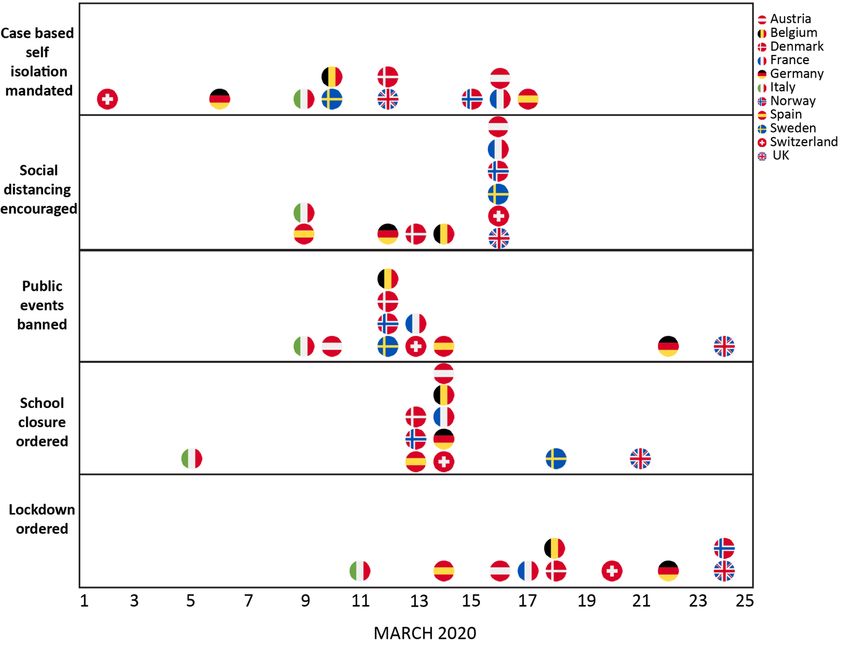
30 March 2020 Imperial College COVID-19 Response Team

In this report, we fit a novel Bayesian mechanistic model of the infection cycle to observed deaths in
11 European countries, inferring plausible upper and lower bounds (Bayesian credible intervals) of the
total populations infected (attack rates), case detection probabilities, and the reproduction number
over time (Rt). We fit the model jointly to COVID-19 data from all these countries to assess whether
there is evidence that interventions have so far been successful at reducing Rt below 1, with the strong
assumption that particular interventions are achieving a similar impact in different countries and that
the efficacy of those interventions remains constant over time. The model is informed more strongly
by countries with larger numbers of deaths and which implemented interventions earlier, therefore
estimates of recent Rt in countries with more recent interventions are contingent on similar
intervention impacts. Data in the coming weeks will enable estimation of country-specific Rt with
greater precision.
Model and data details are presented in the appendix, validation and sensitivity are also presented in
the appendix, and general limitations presented below in the conclusions.

2 Results
The timing of interventions should be taken in the context of when an individual country’s epidemic
started to grow along with the speed with which control measures were implemented. Italy was the
first to begin intervention measures, and other countries followed soon afterwards (Figure 1). Most
interventions began around 12th-14th March. We analyzed data on deaths up to 28th March, giving a
2-3-week window over which to estimate the effect of interventions. Currently, most countries in our
study have implemented all major non-pharmaceutical interventions.
For each country, we model the number of infections, the number of deaths, and , the effective
reproduction number over time, with changing only when an intervention is introduced (Figure 2-
12). is the average number of secondary infections per infected individual, assuming that the
interventions that are in place at time t stay in place throughout their entire infectious period. Every
country has its own individual starting reproduction number before interventions take place.
Specific interventions are assumed to have the same relative impact on in each country when they
were introduced there and are informed by mortality data across all countries.

DOI: Page 4 of 35

30 March 2020 Imperial College COVID-19 Response Team

Figure 1: Intervention timings for the 11 European countries included in the analysis. For further
details see Appendix 8.6.

2.1 Estimated true numbers of infections and current attack rates
In all countries, we estimate there are orders of magnitude fewer infections detected (Figure 2) than
true infections, mostly likely due to mild and asymptomatic infections as well as limited testing
capacity. In Italy, our results suggest that, cumulatively, 5.9 [1.9-15.2] million people have been
infected as of March 28th, giving an attack rate of 9.8% [3.2%-25%] of the population (Table 1). Spain
has recently seen a large increase in the number of deaths, and given its smaller population, our model
estimates that a higher proportion of the population, 15.0% (7.0 [1.8-19] million people) have been
infected to date. Germany is estimated to have one of the lowest attack rates at 0.7% with 600,000
[240,000-1,500,000] people infected.

DOI: Page 5 of 35

30 March 2020 Imperial College COVID-19 Response Team

Table 1: Posterior model estimates of percentage of total population infected as of 28th March 2020.

 Country % of total population infected (mean [95% credible interval])
 Austria 1.1% [0.36%-3.1%]
 Belgium 3.7% [1.3%-9.7%]
 Denmark 1.1% [0.40%-3.1%]
 France 3.0% [1.1%-7.4%]
 Germany 0.72% [0.28%-1.8%]
 Italy 9.8% [3.2%-26%]
 Norway 0.41% [0.09%-1.2%]
 Spain 15% [3.7%-41%]
 Sweden 3.1% [0.85%-8.4%]
 Switzerland 3.2% [1.3%-7.6%]
 United Kingdom 2.7% [1.2%-5.4%]

2.2 Reproduction numbers and impact of interventions
Averaged across all countries, we estimate initial reproduction numbers of around 3.87 [3.01-4.66],
which is in line with other estimates.1,8 These estimates are informed by our choice of serial interval
distribution and the initial growth rate of observed deaths. A shorter assumed serial interval results in
lower starting reproduction numbers (Appendix 8.4.2, Appendix 8.4.6). The initial reproduction
numbers are also uncertain due to (a) importation being the dominant source of new infections early
in the epidemic, rather than local transmission (b) possible under-ascertainment in deaths particularly
before testing became widespread.
We estimate large changes in in response to the combined non-pharmaceutical interventions. Our
results, which are driven largely by countries with advanced epidemics and larger numbers of deaths
(e.g. Italy, Spain), suggest that these interventions have together had a substantial impact on
transmission, as measured by changes in the estimated reproduction number Rt. Across all countries
we find current estimates of Rt to range from a posterior mean of 0.97 [0.14-2.14] for Norway to a
posterior mean of 2.64 [1.40-4.18] for Sweden, with an average of 1.43 across the 11 country posterior
means, a 64% reduction compared to the pre-intervention values. We note that these estimates are
contingent on intervention impact being the same in different countries and at different times. In all
countries but Sweden, under the same assumptions, we estimate that the current reproduction
number includes 1 in the uncertainty range. The estimated reproduction number for Sweden is higher,
not because the mortality trends are significantly different from any other country, but as an artefact
of our model, which assumes a smaller reduction in Rt because no full lockdown has been ordered so
far. Overall, we cannot yet conclude whether current interventions are sufficient to drive below 1
(posterior probability of being less than 1.0 is 44% on average across the countries). We are also
unable to conclude whether interventions may be different between countries or over time.
There remains a high level of uncertainty in these estimates. It is too early to detect substantial
intervention impact in many countries at earlier stages of their epidemic (e.g. Germany, UK, Norway).
Many interventions have occurred only recently, and their effects have not yet been fully observed
due to the time lag between infection and death. This uncertainty will reduce as more data become
available. For all countries, our model fits observed deaths data well (Bayesian goodness of fit tests).
We also found that our model can reliably forecast daily deaths 3 days into the future, by withholding
the latest 3 days of data and comparing model predictions to observed deaths (Appendix 8.3).
The close spacing of interventions in time made it statistically impossible to determine which had the
greatest effect (Figure 1, Figure 4). However, when doing a sensitivity analysis (Appendix 8.4.3) with
uninformative prior distributions (where interventions can increase deaths) we find similar impact of

DOI: Page 6 of 35

30 March 2020 Imperial College COVID-19 Response Team

interventions, which shows that our choice of prior distribution is not driving the effects we see in the
main analysis.

(A) Austria

(B) Belgium

(C) Denmark

(D) France

DOI: Page 7 of 35

30 March 2020 Imperial College COVID-19 Response Team

(E) Germany

(F) Italy

(G) Norway

(H) Spain

DOI: Page 8 of 35

30 March 2020 Imperial College COVID-19 Response Team

(I) Sweden

(J) Switzerland

(K) United Kingdom

Figure 2: Country-level estimates of infections, deaths and Rt. Left: daily number of infections, brown
bars are reported infections, blue bands are predicted infections, dark blue 50% credible interval (CI),
light blue 95% CI. The number of daily infections estimated by our model drops immediately after an
intervention, as we assume that all infected people become immediately less infectious through the
intervention. Afterwards, if the Rt is above 1, the number of infections will starts growing again.
Middle: daily number of deaths, brown bars are reported deaths, blue bands are predicted deaths, CI
as in left plot. Right: time-varying reproduction number , dark green 50% CI, light green 95% CI.
Icons are interventions shown at the time they occurred.

DOI: Page 9 of 35

30 March 2020 Imperial College COVID-19 Response Team

Table 2: Total forecasted deaths since the beginning of the epidemic up to 31 March in our model
and in a counterfactual model (assuming no intervention had taken place). Estimated averted deaths
over this time period as a result of the interventions. Numbers in brackets are 95% credible intervals.

 Model Model
 Observed Model estimated Model deaths
 estimated estimated
 Deaths to 28th deaths to 28th averted to 31
 deaths to 31 deaths to 31
 March March March
 March March

 Country
 (counterfactual
 (difference
 model
 between
 (observed) (our model) (our model) assuming no
 counterfactual
 interventions
 and actual)
 have occurred)

 68 88 [57 - 130] 140 [88 - 210] 280 [140 - 140 [34 -
 Austria
 560] 380]
 289 310 [230 - 420] 510 [370 - 1,100 [590 - 560 [160 -
 Belgium
 730] 2,100] 1,500]

 Denmark 52 61 [38 - 92] 93 [58 - 140] 160 [84 - 310] 69 [15 - 200]

 1,995 1,900 [1,500 - 3,100 [2,300 - 5,600 [3,600 - 2,500 [1,000
 France
 2,500] 4,200] 8,500] - 4,800]
 325 320 [240 - 410] 570 [400 - 1,100 [570 - 550 [91 -
 Germany
 810] 2,400] 1,800]
 9,136 10,000 [8,200 - 14,000 52,000 38,000
 Italy 13,000] [11,000 - [27,000 - [13,000 -
 19,000] 98,000] 84,000]
 16 17 [7 - 33] 26 [11 - 51] 36 [14 - 81] 9.9 [0.82 -
 Norway
 38]
 4,858 4,700 [3,700 - 7,700 [5,500 - 24,000 16,000
 Spain 6,100] 11,000] [13,000 - [5,400 -
 44,000] 35,000]
 92 89 [61 - 120] 160 [110 - 240 [140 - 82 [12 - 250]
 Sweden
 240] 440]
 197 190 [140 - 250] 310 [220 - 650 [330 - 340 [71 -
 Switzerland
 440] 1,500] 1,100]
 United 759 810 [610 - 1,500 [1,000 - 1,800 [1,200 - 370 [73 -
 Kingdom 1,100] 2,100] 2,900] 1,000]
 All 17,787 19,000 [16,000 - 28,000 87,000 59,000
 22,000] [23,000 - [53,000 - [21,000 -
 36,000] 140,000] 120,000]

DOI: Page 10 of 35

30 March 2020 Imperial College COVID-19 Response Team

2.3 Estimated impact of interventions on deaths
Table 2 shows total forecasted deaths since the beginning of the epidemic up to and including 31
March under our fitted model and under the counterfactual model, which predicts what would have
happened if no interventions were implemented (and = 0 i.e. the initial reproduction number
estimated before interventions). Again, the assumption in these predictions is that intervention
impact is the same across countries and time. The model without interventions was unable to capture
recent trends in deaths in several countries, where the rate of increase had clearly slowed (Figure 3).
Trends were confirmed statistically by Bayesian leave-one-out cross-validation and the widely
applicable information criterion assessments – WAIC).
By comparing the deaths predicted under the model with no interventions to the deaths predicted in
our intervention model, we calculated the total deaths averted up to the end of March. We find that,
across 11 countries, since the beginning of the epidemic, 59,000 [21,000-120,000] deaths have been
averted due to interventions. In Italy and Spain, where the epidemic is advanced, 38,000 [13,000-
84,000] and 16,000 [5,400-35,000] deaths have been averted, respectively. Even in the UK, which is
much earlier in its epidemic, we predict 370 [73-1,000] deaths have been averted.
These numbers give only the deaths averted that would have occurred up to 31 March. If we were to
include the deaths of currently infected individuals in both models, which might happen after 31
March, then the deaths averted would be substantially higher.

 (a) Italy (b) Spain
Figure 3: Daily number of confirmed deaths, predictions (up to 28 March) and forecasts (after) for (a)
Italy and (b) Spain from our model with interventions (blue) and from the no interventions
counterfactual model (pink); credible intervals are shown one week into the future. Other countries
are shown in Appendix 8.6.

DOI: Page 11 of 35

30 March 2020 Imperial College COVID-19 Response Team

Figure 4: Our model includes five covariates for governmental interventions, adjusting for whether
the intervention was the first one undertaken by the government in response to COVID-19 (red) or
was subsequent to other interventions (green). Mean relative percentage reduction in is shown
with 95% posterior credible intervals. If 100% reduction is achieved, = 0 and there is no more
transmission of COVID-19. No effects are significantly different from any others, probably due to the
fact that many interventions occurred on the same day or within days of each other as shown in
Figure 1.

3 Discussion
During this early phase of control measures against the novel coronavirus in Europe, we analyze trends
in numbers of deaths to assess the extent to which transmission is being reduced. Representing the
COVID-19 infection process using a semi-mechanistic, joint, Bayesian hierarchical model, we can
reproduce trends observed in the data on deaths and can forecast accurately over short time horizons.
We estimate that there have been many more infections than are currently reported. The high level
of under-ascertainment of infections that we estimate here is likely due to the focus on testing in
hospital settings rather than in the community. Despite this, only a small minority of individuals in
each country have been infected, with an attack rate on average of 4.9% [1.9%-11%] with considerable
variation between countries (Table 1). Our estimates imply that the populations in Europe are not
close to herd immunity (~50-75% if R0 is 2-4). Further, with Rt values dropping substantially, the rate
of acquisition of herd immunity will slow down rapidly. This implies that the virus will be able to spread
rapidly should interventions be lifted. Such estimates of the attack rate to date urgently need to be
validated by newly developed antibody tests in representative population surveys, once these become
available.
We estimate that major non-pharmaceutical interventions have had a substantial impact on the time-
varying reproduction numbers in countries where there has been time to observe intervention effects
on trends in deaths (Italy, Spain). If adherence in those countries has changed since that initial period,
then our forecast of future deaths will be affected accordingly: increasing adherence over time will
have resulted in fewer deaths and decreasing adherence in more deaths. Similarly, our estimates of
the impact of interventions in other countries should be viewed with caution if the same interventions
have achieved different levels of adherence than was initially the case in Italy and Spain.
Due to the implementation of interventions in rapid succession in many countries, there are not
enough data to estimate the individual effect size of each intervention, and we discourage attributing

DOI: Page 12 of 35

30 March 2020 Imperial College COVID-19 Response Team

associations to individual intervention. In some cases, such as Norway, where all interventions were
implemented at once, these individual effects are by definition unidentifiable. Despite this, while
individual impacts cannot be determined, their estimated joint impact is strongly empirically justified
(see Appendix 8.4 for sensitivity analysis). While the growth in daily deaths has decreased, due to the
lag between infections and deaths, continued rises in daily deaths are to be expected for some time.
To understand the impact of interventions, we fit a counterfactual model without the interventions
and compare this to the actual model. Consider Italy and the UK - two countries at very different stages
in their epidemics. For the UK, where interventions are very recent, much of the intervention strength
is borrowed from countries with older epidemics. The results suggest that interventions will have a
large impact on infections and deaths despite counts of both rising. For Italy, where far more time has
passed since the interventions have been implemented, it is clear that the model without
interventions does not fit well to the data, and cannot explain the sub-linear (on the logarithmic scale)
reduction in deaths (see Figure 10).
The counterfactual model for Italy suggests that despite mounting pressure on health systems,
interventions have averted a health care catastrophe where the number of new deaths would have
been 3.7 times higher (38,000 deaths averted) than currently observed. Even in the UK, much earlier
in its epidemic, the recent interventions are forecasted to avert 370 total deaths up to 31 of March.

4 Conclusion and Limitations
Modern understanding of infectious disease with a global publicized response has meant that
nationwide interventions could be implemented with widespread adherence and support. Given
observed infection fatality ratios and the epidemiology of COVID-19, major non-pharmaceutical
interventions have had a substantial impact in reducing transmission in countries with more advanced
epidemics. It is too early to be sure whether similar reductions will be seen in countries at earlier
stages of their epidemic. While we cannot determine which set of interventions have been most
successful, taken together, we can already see changes in the trends of new deaths. When forecasting
3 days and looking over the whole epidemic the number of deaths averted is substantial. We note that
substantial innovation is taking place, and new more effective interventions or refinements of current
interventions, alongside behavioral changes will further contribute to reductions in infections. We
cannot say for certain that the current measures have controlled the epidemic in Europe; however, if
current trends continue, there is reason for optimism.
Our approach is semi-mechanistic. We propose a plausible structure for the infection process and then
estimate parameters empirically. However, many parameters had to be given strong prior
distributions or had to be fixed. For these assumptions, we have provided relevant citations to
previous studies. As more data become available and better estimates arise, we will update these in
weekly reports. Our choice of serial interval distribution strongly influences the prior distribution for
starting 0 . Our infection fatality ratio, and infection-to-onset-to-death distributions strongly
influence the rate of death and hence the estimated number of true underlying cases.
We also assume that the effect of interventions is the same in all countries, which may not be fully
realistic. This assumption implies that countries with early interventions and more deaths since these
interventions (e.g. Italy, Spain) strongly influence estimates of intervention impact in countries at
earlier stages of their epidemic with fewer deaths (e.g. Germany, UK).
 We have tried to create consistent definitions of all interventions and document details of this in
Appendix 8.6. However, invariably there will be differences from country to country in the strength of
their intervention – for example, most countries have banned gatherings of more than 2 people when
implementing a lockdown, whereas in Sweden the government only banned gatherings of more than
10 people. These differences can skew impacts in countries with very little data. We believe that our
uncertainty to some degree can cover these differences, and as more data become available,
coefficients should become more reliable.

DOI: Page 13 of 35

30 March 2020 Imperial College COVID-19 Response Team

However, despite these strong assumptions, there is sufficient signal in the data to estimate changes
in (see the sensitivity analysis reported in Appendix 8.4.3) and this signal will stand to increase with
time. In our Bayesian hierarchical framework, we robustly quantify the uncertainty in our parameter
estimates and posterior predictions. This can be seen in the very wide credible intervals in more recent
days, where little or no death data are available to inform the estimates. Furthermore, we predict
intervention impact at country-level, but different trends may be in place in different parts of each
country. For example, the epidemic in northern Italy was subject to controls earlier than the rest of
the country.

5 Data
Our model utilizes daily real-time death data from the ECDC (European Centre of Disease Control),
where we catalogue case data for 11 European countries currently experiencing the epidemic: Austria,
Belgium, Denmark, France, Germany, Italy, Norway, Spain, Sweden, Switzerland and the United
Kingdom. The ECDC provides information on confirmed cases and deaths attributable to COVID-19.
However, the case data are highly unrepresentative of the incidence of infections due to
underreporting as well as systematic and country-specific changes in testing.
We, therefore, use only deaths attributable to COVID-19 in our model; we do not use the ECDC case
estimates at all. While the observed deaths still have some degree of unreliability, again due to
changes in reporting and testing, we believe the data are of sufficient fidelity to model. For population
counts, we use UNPOP age-stratified counts.10
We also catalogue data on the nature and type of major non-pharmaceutical interventions. We looked
at the government webpages from each country as well as their official public health
division/information webpages to identify the latest advice/laws being issued by the government and
public health authorities. We collected the following:
School closure ordered: This intervention refers to nationwide extraordinary school closures which in
most cases refer to both primary and secondary schools closing (for most countries this also includes
the closure of other forms of higher education or the advice to teach remotely). In the case of Denmark
and Sweden, we allowed partial school closures of only secondary schools. The date of the school
closure is taken to be the effective date when the schools started to be closed (if this was on a Monday,
the date used was the one of the previous Saturdays as pupils and students effectively stayed at home
from that date onwards).
Case-based measures: This intervention comprises strong recommendations or laws to the general
public and primary care about self-isolation when showing COVID-19-like symptoms. These also
include nationwide testing programs where individuals can be tested and subsequently self-isolated.
Our definition is restricted to nationwide government advice to all individuals (e.g. UK) or to all primary
care and excludes regional only advice. These do not include containment phase interventions such
as isolation if travelling back from an epidemic country such as China.
Public events banned: This refers to banning all public events of more than 100 participants such as
sports events.
Social distancing encouraged: As one of the first interventions against the spread of the COVID-19
pandemic, many governments have published advice on social distancing including the
recommendation to work from home wherever possible, reducing use of public transport and all other
non-essential contact. The dates used are those when social distancing has officially been
recommended by the government; the advice may include maintaining a recommended physical
distance from others.
Lockdown decreed: There are several different scenarios that the media refers to as lockdown. As an
overall definition, we consider regulations/legislations regarding strict face-to-face social interaction:
including the banning of any non-essential public gatherings, closure of educational and

DOI: Page 14 of 35

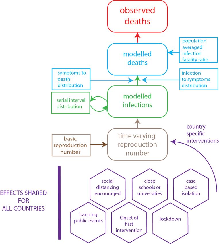
30 March 2020 Imperial College COVID-19 Response Team

public/cultural institutions, ordering people to stay home apart from exercise and essential tasks. We
include special cases where these are not explicitly mentioned on government websites but are
enforced by the police (e.g. France). The dates used are the effective dates when these legislations
have been implemented. We note that lockdown encompasses other interventions previously
implemented.
First intervention: As Figure 1 shows, European governments have escalated interventions rapidly,
and in some examples (Norway/Denmark) have implemented these interventions all on a single day.
Therefore, given the temporal autocorrelation inherent in government intervention, we include a
binary covariate for the first intervention, which can be interpreted as a government decision to take
major action to control COVID-19.
A full list of the timing of these interventions and the sources we have used can be found in Appendix
8.6.

6 Methods Summary
A visual summary of our model is presented in Figure 5 (details in Appendix 8.1 and 8.2). Replication
code is available at https://github.com/ImperialCollegeLondon/covid19model/releases/tag/v1.0
We fit our model to observed deaths according to ECDC data from 11 European countries. The
modelled deaths are informed by an infection-to-onset distribution (time from infection to the onset
of symptoms), an onset-to-death distribution (time from the onset of symptoms to death), and the
population-averaged infection fatality ratio (adjusted for the age structure and contact patterns of
each country, see Appendix). Given these distributions and ratios, modelled deaths are a function of
the number of infections. The modelled number of infections is informed by the serial interval
distribution (the average time from infection of one person to the time at which they infect another)
and the time-varying reproduction number. Finally, the time-varying reproduction number is a
function of the initial reproduction number before interventions and the effect sizes from
interventions.

DOI: Page 15 of 35

30 March 2020 Imperial College COVID-19 Response Team

Figure 5: Summary of model components.

Following the hierarchy from bottom to top gives us a full framework to see how interventions affect
infections, which can result in deaths. We use Bayesian inference to ensure our modelled deaths can
reproduce the observed deaths as closely as possible. From bottom to top in Figure 5, there is an
implicit lag in time that means the effect of very recent interventions manifest weakly in current
deaths (and get stronger as time progresses). To maximise the ability to observe intervention impact
on deaths, we fit our model jointly for all 11 European countries, which results in a large data set. Our
model jointly estimates the effect sizes of interventions. We have evaluated the effect of our Bayesian
prior distribution choices and evaluate our Bayesian posterior calibration to ensure our results are
statistically robust (Appendix 8.4).

7 Acknowledgements
Initial research on covariates in Appendix 8.6 was crowdsourced; we thank a number of people
across the world for help with this. This work was supported by Centre funding from the UK Medical
Research Council under a concordat with the UK Department for International Development, the
NIHR Health Protection Research Unit in Modelling Methodology and Community Jameel.

DOI: Page 16 of 35

30 March 2020 Imperial College COVID-19 Response Team

8 Appendix: Model Specifics, Validation and Sensitivity Analysis
8.1 Death model
We observe daily deaths , for days t ∈ 1, … , n and countries m ∈ 1, … , p. These daily deaths are
modelled using a positive real-valued function , = E( , ) that represents the expected number
of deaths attributed to COVID-19. , is assumed to follow a negative binomial distribution with
 , 2
mean , and variance , + ψ
 , where ψ follows a half normal distribution, i.e.

 , 2
 , ∼ Negative Binomial ( , , , + ),
 ψ
 ψ ∼ orma + (0,5).
The expected number of deaths d in a given country on a given day is a function of the number of
infections c occurring in previous days.
At the beginning of the epidemic, the observed deaths in a country can be dominated by deaths that
result from infection that are not locally acquired. To avoid biasing our model by this, we only include
observed deaths from the day after a country has cumulatively observed 10 deaths in our model.
To mechanistically link our function for deaths to infected cases, we use a previously estimated COVID-
19 infection-fatality-ratio ifr (probability of death given infection)9 together with a distribution of times
from infection to death π. The ifr is derived from estimates presented in Verity et al11 which assumed
homogeneous attack rates across age-groups. To better match estimates of attack rates by age
generated using more detailed information on country and age-specific mixing patterns, we scale
these estimates (the unadjusted ifr, referred to here as ifr’) in the following way as in previous work.4
Let be the number of infections generated in age-group a, the underlying size of the population
in that age group and A = / the age-group-specific attack rate. The adjusted ifr is then given
 50−59
by: if = if ′ , where A 50−59 is the predicted attack-rate in the 50-59 year age-group after
 
incorporating country-specific patterns of contact and mixing. This age-group was chosen as the
reference as it had the lowest predicted level of underreporting in previous analyses of data from the
Chinese epidemic11. We obtained country-specific estimates of attack rate by age, A , for the 11
European countries in our analysis from a previous study which incorporates information on contact
between individuals of different ages in countries across Europe.12 We then obtained overall ifr
estimates for each country adjusting for both demography and age-specific attack rates.
Using estimated epidemiological information from previous studies,4,11 we assume π to be the sum of
two independent random times: the incubation period (infection to onset of symptoms or infection-
to-onset) distribution and the time between onset of symptoms and death (onset-to-death). The
infection-to-onset distribution is Gamma distributed with mean 5.1 days and coefficient of variation
0.86. The onset-to-death distribution is also Gamma distributed with a mean of 18.8 days and a
coefficient of variation 0.45. if is population averaged over the age structure of a given country. The
infection-to-death distribution is therefore given by:
 π ∼ f ⋅ (Gamma(5.1,0.86) + Gamma(18.8,0.45))
Figure 6 shows the infection-to-death distribution and the resulting survival function that integrates
to the infection fatality ratio.

DOI: Page 17 of 35

30 March 2020 Imperial College COVID-19 Response Team

Figure 6: Left, infection-to-death distribution (mean 23.9 days). Right, survival probability of infected
individuals per day given the infection fatality ratio (1%) and the infection-to-death distribution on
the left.

Using the probability of death distribution, the expected number of deaths , , on a given day t, for
country, m, is given by the following discrete sum:
 , = ∑ −1
 τ=0 τ, π −τ, ,

where τ, is the number of new infections on day τ in country m (see next section) and where π is
 +0.5 1.5
discretized via π , = ∫τ= −0.5 π (τ)d for s = 2,3, … and π1, = ∫τ=0 π (τ)d.
The number of deaths today is the sum of the past infections weighted by their probability of death,
where the probability of death depends on the number of days since infection.

8.2 Infection model
The true number of infected individuals, c, is modelled using a discrete renewal process. This approach
has been used in numerous previous studies13–16 and has a strong theoretical basis in stochastic
individual-based counting processes such as Hawkes process and the Bellman-Harris process.17,18 The
renewal model is related to the Susceptible-Infected-Recovered model, except the renewal is not
expressed in differential form. To model the number of infections over time we need to specify a serial
interval distribution g with density g(τ), (the time between when a person gets infected and when
they subsequently infect another other people), which we choose to be Gamma distributed:
 g ∼ amma (6.5,0.62).
The serial interval distribution is shown below in Figure 7 and is assumed to be the same for all
countries.

DOI: Page 18 of 35

30 March 2020 Imperial College COVID-19 Response Team

Figure 7: Serial interval distribution with a mean of 6.5 days.

Given the serial interval distribution, the number of infections , on a given day t, and country, m,
is given by the following discrete convolution function:
 , = , ∑ −1
 τ=0 τ, −τ ,

where, similar to the probability of death function, the daily serial interval is discretized by
 +0.5 1.5
 = ∫τ= −0.5 (τ)dτ for s = 2,3, … and 1 = ∫τ=0 (τ)d .
Infections today depend on the number of infections in the previous days, weighted by the discretized
serial interval distribution. This weighting is then scaled by the country-specific time-varying
reproduction number, , , that models the average number of secondary infections at a given time.
The functional form for the time-varying reproduction number was chosen to be as simple as possible
to minimize the impact of strong prior assumptions: we use a piecewise constant function that scales
 , from a baseline prior 0, and is driven by known major non-pharmaceutical interventions
occurring in different countries and times. We included 6 interventions, one of which is constructed
from the other 5 interventions, which are timings of school and university closures (k=1), self-isolating
if ill (k=2), banning of public events (k=3), any government intervention in place (k=4), implementing
a partial or complete lockdown (k=5) and encouraging social distancing and isolation (k=6). We denote
the indicator variable for intervention k ∈ 1,2,3,4,5,6 by , , , which is 1 if intervention k is in place
in country m at time t and 0 otherwise. The covariate “any government intervention” (k=4) indicates
if any of the other 5 interventions are in effect, i.e. 4, , equals 1 at time t if any of the interventions
k ∈ 1,2,3,4,5 are in effect in country m at time t and equals 0 otherwise. Covariate 4 has the
interpretation of indicating the onset of major government intervention. The effect of each
intervention is assumed to be multiplicative. , is therefore a function of the intervention indicators
 , , in place at time t in country m:
 , = 0, exp(− ∑6 =1 α , , ).
The exponential form was used to ensure positivity of the reproduction number, with 0, 
constrained to be positive as it appears outside the exponential. The impact of each intervention on
 , is characterised by a set of parameters α1 , … , α6 , with independent prior distributions chosen
to be

DOI: Page 19 of 35

30 March 2020 Imperial College COVID-19 Response Team

 α ∼ amma(. 5,1).
The impacts α are shared between all m countries and therefore they are informed by all available
data. The prior distribution for 0 was chosen to be
 0, ∼ ormal(2.4, |κ|) with κ ∼ ormal(0,0.5),
Once again, κ is the same among all countries to share information.
We assume that seeding of new infections begins 30 days before the day after a country has
cumulatively observed 10 deaths. From this date, we seed our model with 6 sequential days of
infections drawn from c1, , … , 6, ~Exponential(τ), where τ~Exponential(0.03). These seed
infections are inferred in our Bayesian posterior distribution.
We estimated parameters jointly for all 11 countries in a single hierarchical model. Fitting was done
in the probabilistic programming language Stan,19 using an adaptive Hamiltonian Monte Carlo (HMC)
sampler. We ran 8 chains for 4000 iterations with 2000 iterations of warmup and a thinning factor 4
to obtain 2000 posterior samples. Posterior convergence was assessed using the Rhat statistic and by
diagnosing divergent transitions of the HMC sampler. Prior-posterior calibrations were also performed
(see below).

8.3 Validation
We validate accuracy of point estimates of our model using cross-validation. In our cross-validation
scheme, we leave out 3 days of known death data (non-cumulative) and fit our model. We forecast
what the model predicts for these three days. We present the individual forecasts for each day, as
well as the average forecast for those three days. The cross-validation results are shown in the Figure
8.

Figure 8: Cross-validation results for 3-day and 3-day aggregated forecasts

Figure 8 provides strong empirical justification for our model specification and mechanism. Our
accurate forecast over a three-day time horizon suggests that our fitted estimates for are
appropriate and plausible.
Along with from point estimates we all evaluate our posterior credible intervals using the Rhat
statistic. The Rhat statistic measures whether our Markov Chain Monte Carlo (MCMC) chains have

DOI: Page 20 of 35

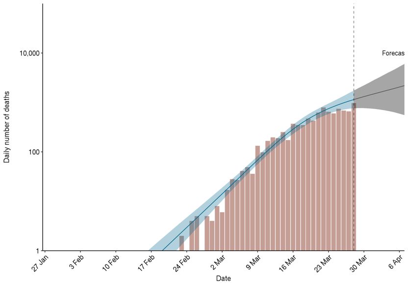
30 March 2020 Imperial College COVID-19 Response Team

converged to the equilibrium distribution (the correct posterior distribution). Figure 9 shows the Rhat
statistics for all of our parameters

Figure 9: Rhat statistics - values close to 1 indicate MCMC convergence.

Figure 9 indicates that our MCMC have converged. In fitting we also ensured that the MCMC sampler
experienced no divergent transitions - suggesting non pathological posterior topologies.

8.4 Sensitivity Analysis
8.4.1 Forecasting on log-linear scale to assess signal in the data
As we have highlighted throughout in this report, the lag between deaths and infections means that
it takes time for information to propagate backwards from deaths to infections, and ultimately to .
A conclusion of this report is the prediction of a slowing of in response to major interventions. To
gain intuition that this is data driven and not simply a consequence of highly constrained model
assumptions, we show death forecasts on a log-linear scale. On this scale a line which curves below a
linear trend is indicative of slowing in the growth of the epidemic. Figure 10 to Figure 12 show these
forecasts for Italy, Spain and the UK. They show this slowing down in the daily number of deaths. Our
model suggests that Italy, a country that has the highest death toll of COVID-19, will see a slowing in
the increase in daily deaths over the coming week compared to the early stages of the epidemic.

DOI: Page 21 of 35

30 March 2020 Imperial College COVID-19 Response Team

Figure 10: 7-day-ahead forecast for Italy.

Figure 11: 7-day-ahead forecast for Spain.

Figure 12: 7-day-ahead forecast for the UK.

DOI: Page 22 of 35

30 March 2020 Imperial College COVID-19 Response Team

8.4.2 Serial interval distribution
We investigated the sensitivity of our estimates of starting and final to our assumed serial interval
distribution. For this we considered several scenarios, in which we changed the serial interval
distribution mean, from a value of 6.5 days, to have values of 5, 6, 7 and 8 days.
In Figure 13, we show our estimates of 0 , the starting reproduction number before interventions, for
each of these scenarios. The relative ordering of the =0 in the countries is consistent in all settings.
However, as expected, the scale of =0 is considerably affected by this change – a longer serial
interval results in a higher estimated =0 . This is because to reach the currently observed size of the
epidemics, a longer assumed serial interval is compensated by a higher estimated 0 .
Additionally, in Figure 14, we show our estimates of at the most recent model time point, again for
each of these scenarios. The serial interval mean can influence substantially, however, the posterior
credible intervals of are broadly overlapping.

Figure 13: Initial reproduction number for different serial interval (SI) distributions (means
between 5 and 8 days). We use 6.5 days in our main analysis.

DOI: Page 23 of 35

30 March 2020 Imperial College COVID-19 Response Team

Figure 14: Rt on 28 March 2020 estimated for all countries, with serial interval (SI) distribution means
between 5 and 8 days. We use 6.5 days in our main analysis.

8.4.3 Uninformative prior sensitivity on α
We ran our model using implausible uninformative prior distributions on the intervention effects,
allowing the effect of an intervention to increase or decrease . To avoid collinearity, we ran 6
separate models, with effects summarized below (compare with the main analysis in Figure 4). In this
series of univariate analyses, we find (Figure 15) that all effects on their own serve to decrease .
This gives us confidence that our choice of prior distribution is not driving the effects we see in the
main analysis. Lockdown has a very large effect, most likely due to the fact that it occurs after other
interventions in our dataset. The relatively large effect sizes for the other interventions are most likely
due to the coincidence of the interventions in time, such that one intervention is a proxy for a few
others.

Figure 15: Effects of different interventions when used as the only covariate in the model.

DOI: Page 24 of 35

30 March 2020 Imperial College COVID-19 Response Team

8.4.4 Nonparametric fitting of using a Gaussian process:
To assess prior assumptions on our piecewise constant functional form for we test using a
nonparametric function with a Gaussian process prior distribution. We fit a model with a Gaussian
process prior distribution to data from Italy where there is the largest signal in death data. We find
that the Gaussian process has a very similar trend to the piecewise constant model and reverts to the
mean in regions of no data. The correspondence of a completely nonparametric function and our
piecewise constant function suggests a suitable parametric specification of .

8.4.5 Leave country out analysis
Due to the different lengths of each European countries’ epidemic, some countries, such as Italy have
much more data than others (such as the UK). To ensure that we are not leveraging too much
information from any one country we perform a “leave one country out” sensitivity analysis, where
we rerun the model without a different country each time. Figure 16 and Figure 17 are examples for
results for the UK, leaving out Italy and Spain. In general, for all countries, we observed no significant
dependence on any one country.

Figure 16: Model results for the UK, when not using data from Italy for fitting the model. See the
caption of Figure 2 for an explanation of the plots.

Figure 17: Model results for the UK, when not using data from Spain for fitting the model. See caption
of Figure 2 for an explanation of the plots.

8.4.6 Starting reproduction numbers vs theoretical predictions
To validate our starting reproduction numbers, we compare our fitted values to those theoretically
expected from a simpler model assuming exponential growth rate, and a serial interval distribution
mean. We fit a linear model with a Poisson likelihood and log link function and extracting the daily
growth rate . For well-known theoretical results from the renewal equation, given a serial interval
distribution ( ) with mean and standard deviation , given = 2 / 2 and = / 2 , and

DOI: Page 25 of 35

30 March 2020 Imperial College COVID-19 Response Team

subsequently 0 = (1 + ) . Figure 18 shows theoretically derived 0 along with our fitted
estimates of =0 from our Bayesian hierarchical model. As shown in Figure 18 there is large
correspondence between our estimated starting reproduction number and the basic reproduction
number implied by the growth rate .

Figure 18: Our estimated ( ) versus theoretically derived ( ) from a log-linear
regression fit.

DOI: Page 26 of 35

30 March 2020 Imperial College COVID-19 Response Team

8.5 Counterfactual analysis – interventions vs no interventions
Figures in this section are all country-specific plots equivalent to Figure 3 which only shows Italy and
Spain.

DOI: Page 27 of 35

30 March 2020 Imperial College COVID-19 Response Team

Figure 19: Daily number of confirmed deaths, predictions (up to 28 March) and forecasts (after) for
all countries except Italy and Spain from our model with interventions (blue) and from the no
interventions counterfactual model (pink); credible intervals are shown one week into the future.

DOI: Page 28 of 35

30 March 2020 Imperial College COVID-19 Response Team

8.6 Data sources and Timeline of Interventions
Figure 1 and Table 3 display the interventions by the 11 countries in our study and the dates these
interventions became effective.
Table 3: Timeline of Interventions.

Country Type Event Date effective
 School closure
 ordered Nationwide school closures. 20 14/3/2020
 Public events
 banned Banning of gatherings of more than 5 people.21 10/3/2020
 Banning all access to public spaces and gatherings
 Lockdown of more than 5 people. Advice to maintain 1m
 ordered distance.22 16/3/2020
 Social distancing
 encouraged Recommendation to maintain a distance of 1m.22 16/3/2020
 Case-based
Austria measures Implemented at lockdown.22 16/3/2020
 School closure
 ordered Nationwide school closures.23 14/3/2020
 Public events All recreational activities cancelled regardless of
 banned size.23 12/3/2020
 Citizens are required to stay at home except for
 Lockdown work and essential journeys. Going outdoors only
 ordered with household members or 1 friend.24 18/3/2020
 Public transport recommended only for essential
 Social distancing journeys, work from home encouraged, all public
 encouraged places e.g. restaurants closed.23 14/3/2020
 Case-based Everyone should stay at home if experiencing a
Belgium measures cough or fever.25 10/3/2020
 School closure Secondary schools shut and universities (primary
 ordered schools also shut on 16th).26 13/3/2020
 Public events Bans of events >100 people, closed cultural
 banned institutions, leisure facilities etc.27 12/3/2020
 Lockdown Bans of gatherings of >10 people in public and all
 ordered public places were shut.27 18/3/2020
 Limited use of public transport. All cultural
 Social distancing institutions shut and recommend keeping
 encouraged appropriate distance.28 13/3/2020
 Case-based Everyone should stay at home if experiencing a
Denmark measures cough or fever.29 12/3/2020

DOI: Page 29 of 35

30 March 2020 Imperial College COVID-19 Response Team

 School closure
 ordered Nationwide school closures.30 14/3/2020
 Public events
 banned Bans of events >100 people.31 13/3/2020
 Lockdown Everybody has to stay at home. Need a self-
 ordered authorisation form to leave home.32 17/3/2020
 Social distancing
 encouraged Advice at the time of lockdown.32 16/3/2020
 Case-based
France measures Advice at the time of lockdown.32 16/03/2020
 School closure
 ordered Nationwide school closures.33 14/3/2020
 Public events No gatherings of >1000 people. Otherwise
 banned regional restrictions only until lockdown.34 22/3/2020
 Lockdown Gatherings of > 2 people banned, 1.5 m
 ordered distance.35 22/3/2020
 Social distancing Avoid social interaction wherever possible
 encouraged recommended by Merkel.36 12/3/2020
 Advice for everyone experiencing symptoms to
 Case-based contact a health care agency to get tested and
Germany measures then self-isolate.37 6/3/2020
 School closure
 ordered Nationwide school closures.38 5/3/2020
 Public events
 banned The government bans all public events.39 9/3/2020
 Lockdown The government closes all public places. People
 ordered have to stay at home except for essential travel.40 11/3/2020
 A distance of more than 1m has to be kept and
 Social distancing any other form of alternative aggregation is to be
 encouraged excluded.40 9/3/2020
 Case-based Advice to self-isolate if experiencing symptoms
Italy measures and quarantine if tested positive.41 9/3/2020
 Norwegian Directorate of Health closes all
 School closure educational institutions. Including childcare
 ordered facilities and all schools.42 13/3/2020
 Public events The Directorate of Health bans all non-necessary
 banned social contact.42 12/3/2020
 Lockdown Only people living together are allowed outside
 ordered together. Everyone has to keep a 2m distance.43 24/3/2020
 Social distancing The Directorate of Health advises against all
 encouraged travelling and non-necessary social contacts.42 16/3/2020
 Case-based Advice to self-isolate for 7 days if experiencing a
Norway measures cough or fever symptoms.44 15/3/2020

DOI: Page 30 of 35