PUBLICATIONS Global Biogeochemical Cycles
←
→
Page content transcription
If your browser does not render page correctly, please read the page content below
PUBLICATIONS
Global Biogeochemical Cycles
RESEARCH ARTICLE                             Changing Amazon biomass and the role
10.1002/2015GB005135
                                             of atmospheric CO2 concentration,
Special Section:                             climate, and land use
Trends and Determinants of
the Amazon Rainforests in a                  Andrea D. de Almeida Castanho1,2, David Galbraith3, Ke Zhang4,5, Michael T. Coe2,
Changing World, A Carbon                     Marcos H. Costa6, and Paul Moorcroft5
Cycle Perspective
                                             1
                                              Department of Agricultural Engineering, Universidade Federal do Ceará, Ceará, Brazil, 2Woods Hole Research Center,
Key Points:                                  Falmouth, Massachusetts, USA, 3School of Geography, University of Leeds, Leeds, UK, 4Cooperative Institute for Mesoscale
• CO2 fertilization is a major contributor   Meteorological Studies, University of Oklahoma, Norman, Oklahoma, USA, 5Department of Organismic and Evolutionary
  to the increase in simulated biomass       Biology, Harvard University, Cambridge, Massachusetts, USA, 6Department of Agricultural Engineering, Universidade
  of old growth forests in the last
                                             Federal de Viçosa, Viçosa, Brazil
  40 years
• Land use change reduces the simulated
  Amazon biomass comparable in
  magnitude to the biomass increase          Abstract The Amazon tropical evergreen forest is an important component of the global carbon budget. Its
  from CO2 fertilization                     forest floristic composition, structure, and function are sensitive to changes in climate, atmospheric composition,
• Better representation of mortality         and land use. In this study biomass and productivity simulated by three dynamic global vegetation models
  from extreme climate events is
  required in DGVMs                          (Integrated Biosphere Simulator, Ecosystem Demography Biosphere Model, and Joint UK Land Environment
                                             Simulator) for the period 1970–2008 are compared with observations from forest plots (Rede Amazónica de
                                             Inventarios Forestales). The spatial variability in biomass and productivity simulated by the DGVMs is low in
                                             comparison to the field observations in part because of poor representation of the heterogeneity of vegetation
Correspondence to:
A. D. A. Castanho,                           traits within the models. We find that over the last four decades the CO2 fertilization effect dominates a long-term
adacastanho@gmail.com                        increase in simulated biomass in undisturbed Amazonian forests, while land use change in the south and
                                             southeastern Amazonia dominates a reduction in Amazon aboveground biomass, of similar magnitude to the
Citation:                                    CO2 biomass gain. Climate extremes exert a strong effect on the observed biomass on short time scales, but the
Castanho, A. D. A., D. Galbraith,            models are incapable of reproducing the observed impacts of extreme drought on forest biomass. We find that
K. Zhang, M. T. Coe, M. H. Costa, and
                                             future improvements in the accuracy of DGVM predictions will require improved representation of four key
P. Moorcroft (2016), Changing Amazon
biomass and the role of atmospheric CO2      elements: (1) spatially variable plant traits, (2) soil and nutrients mediated processes, (3) extreme event mortality,
concentration, climate, and land use,        and (4) sensitivity to climatic variability. Finally, continued long-term observations and ecosystem-scale
Global Biogeochem. Cycles, 30, 18–39,
                                             experiments (e.g. Free-Air CO2 Enrichment experiments) are essential for a better understanding of the
doi:10.1002/2015GB005135.
                                             changing dynamics of tropical forests.
Received 6 MAR 2015
Accepted 29 OCT 2015
Accepted article online 6 NOV 2015
Published online 19 JAN 2016                 1. Introduction
                                             Increasing atmospheric CO2, changing climate and land cover/land use change are three important factors acting
                                             on the world’s forests, potentially altering their carbon balance in both positive and negative ways. Increasing
                                             CO2 is expected to boost plant photosynthetic rates directly and also to improve water use efficiency resulting
                                             in an enhancement of terrestrial carbon sinks assuming there are no changes in the allocation of photosynthates
                                             and turnover time of carbon [Lloyd and Farquhar, 1996]. Changing climate can further enhance or diminish ter-
                                             restrial C sinks, depending on water availability and temperature constraints [Reichstein et al., 2013; Zscheischler
                                             et al., 2014]. Furthermore, at larger spatial scales land use change exerts a strong control on the regional C bal-
                                             ance as large swathes of the world’s major biomes have been converted for agricultural use [Foley et al., 2011].
                                             Spanning an area of ~7 × 10⁶km2, the Amazon forest is thought to be a significant atmospheric carbon sink
                                             [Phillips et al., 2008]. Given their size, any widespread changes in the C balance of Amazonian forests could
                                             directly affect global climate and have important implications for mitigation policies designed to stabilize
                                             greenhouse gases levels [Aragão et al., 2014; Houghton, 2014; Pan et al., 2011]. Thus, accurate understanding
                                             and representations of the response of tropical forests to changing environmental resources (atmospheric
                                             CO2 concentrations, temperature, water availabilitys, nutrients, and light) and land use change are essential
                                             for robust future predictions of the global carbon cycle.

©2015. American Geophysical Union.           Long-term forest inventory studies of old-growth forests across Amazonia have documented an increase
All Rights Reserved.                         in aboveground biomass in recent decades [Baker et al., 2004; Lewis et al., 2004c; Phillips et al., 2008;

CASTANHO ET AL.                                                         CHANGING AMAZON BIOMASS                                                                   18
Global Biogeochemical Cycles                                                          10.1002/2015GB005135

                      Phillips et al., 1998]. The authors of these studies have pointed to increasing atmospheric CO2 as the most likely
                      driver of the observed Amazonian forest carbon sink. Other possible drivers that have been highlighted include
                      climate variations, increasing nutrient mineralization rates, and increases in diffuse radiation due to increasing
                      atmospheric aerosol loads resulting from biomass burning; each of these possibilities are discussed in detail in
                      [Lewis et al., 2004b, 2009]. Another hypothesis suggests that the increase in biomass could be a recovery from
                      large-scale past disturbances, such as drought [Clark et al., 2010; Muller-Landau, 2009; Wright, 2013]. Although
                      this may be true for specific monitoring sites across the study area (as for example in Tapajos in Brazilian
                      Amazonia), [Lewis et al., 2004c], the very long return times of such disturbance events across the study area
                      makes their large-scale impact less clear [Espirito-Santo et al., 2014].
                      In this study dynamic global vegetation models (DGVMs) are used to explore the contributions of CO2,
                      climate, and land use to changes in the Amazonian C balance between 1970 and 2008. While DGVMs have
                      frequently been used in assessments of the impacts of future climate change on Amazonian forests
                      [Galbraith et al., 2010; Huntingford et al., 2013; Rammig et al., 2010; Zhang et al., 2015], there has been little
                      evaluation of their ability to simulate biomass dynamics as observed by field measurements. Forest plot data
                      on biomass dynamics reflect the contributions of several external forces, including short and long-term
                      climate variability and disturbances (e.g., fire and blowdown events) as well as long-term increases in
                      atmospheric CO2 concentration. DGVMs can help to separate the individual effects of climate, increasing
                      atmospheric CO2 concentrations, land use change or fire, on carbon stocks, and fluxes. In undisturbed forests,
                      where long-term measurement plots are located, DGVMs provide a test for the hypothesis that CO2
                      fertilization is the major mechanism driving the observed increase in biomass of undisturbed forest plots.
                      In this study, a suite of simulations is conducted using three DGVMs to isolate the individual and combined
                      effects of CO2, climate, and land use change on the long-term Amazonian C balance (1970–2008). The ability
                      of the DGVMs to reproduce biomass responses to long-term (e.g., decadal climatic variation) and short-term
                      (e.g., single-year drought events) forcings is evaluated.

                      2. Material and Methods
                      2.1. Dynamic Global Vegetation Models Description
                      We use three Dynamic Global Vegetation Models (DGVM): the Integrated Biosphere Simulator (IBIS) [Foley
                      et al., 1996; Kucharik et al., 2000], the Ecosystem Demography Biosphere Model (ED2) [Medvigy et al., 2009;
                      Moorcroft et al., 2001], and the Joint UK Land Environment Simulator Model (JULES, v2.1) [Best et al., 2011;
                      Clark et al., 2011]. IBIS, and JULES simulate community dynamics and competition between plant functional
                      types (PFTs) using an aggregated “big-leaf” representation of the plant canopy within each climatological
                      grid cell. ED2 represents tree population, size and age structure explicitly, simulating individual plant-scale
                      dynamics and competition. A summary of the exclusive processes and parameterizations that the models
                      use is described below and is summarized in Table 1; detailed additional information on the C3 plant physio-
                      logical processes are described in Tables A1 and A2 in Appendix A. The basic functions are the same between
                      the models; however, parameterization and specific factors that modulate photosynthesis and stomatal
                      conductance, such as water stress factors and phenology differ between the models, causing differences
                      in simulated vegetation sensitivity to CO2 fertilization and water stress. A detailed description of the models
                      can be found in the original model description papers.
                      2.2. Numerical Models Simulations Protocol
                      The application of all DGVMs followed a common protocol, being forced with the same climate and soil con-
                      ditions [Zhang et al., 2015]. The region of study was delimited by the Amazon watershed and the Guiana
                      Shield region to the north, with a total area of 8 × 10⁶ km2 (Figure 1). The simulations were made at 1 × 1° hor-
                      izontal spatial resolution with an hourly time step for the 39 year period from 1970 to 2008. During this period
                      the models were forced with prescribed hourly climate based on the Sheffield et al. [2006] database, which is a
                      combination of global observation-based data sets and reanalysis data from the National Center for
                      Environmental Prediction-National Center for Atmospheric Research. The year 1970 was chosen as a start
                      date of our analysis because it is the point at which the weather station network over Amazonia was suffi-
                      ciently dense to provide reliable climate records [Costa et al., 2009]. Atmospheric CO2 concentrations were
                      generated by fitting an exponential function to the ice core data (1700–1959) concatenated with the
                      observed CO2 concentrations for the historical period (1959–2008) [Zhang et al., 2015]. All DGVMs followed

CASTANHO ET AL.                                CHANGING AMAZON BIOMASS                                                               19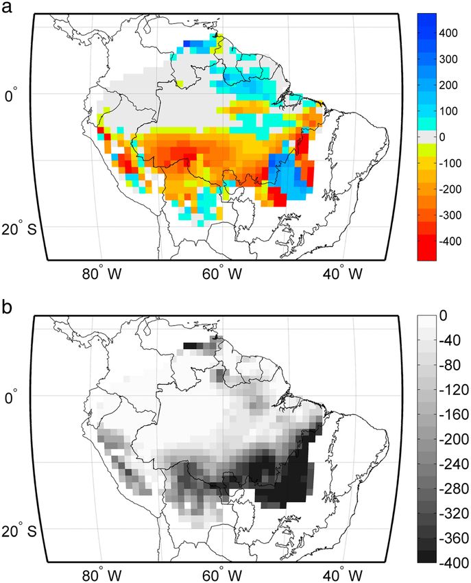
Global Biogeochemical Cycles                                                                        10.1002/2015GB005135

Table 1. Summary of Relevant Properties and Processes of the DGVMs Used in This Study
                                                         IBIS                                            ED2                                          JULES

                                                                                  Processes
Representation of plant canopy                      Big-leaf                           Size and age-structured individual scale                    Big-leaf
Plant functional types                 Tropical broadleaf evergreen trees;           Tropical plant functional type: fast-growing         Broadleaf evergreen trees;
                                       Tropical broadleaf deciduous trees;              pioneer tropical trees; midsuccessional           shrubs; C3 and C4 grasses
                                             shrubs; C3, C4 grasses                  tropical trees; slow-growing, shade-tolerant
                                                                                        late successional trees; C3 grasses and
                                                                                            forbs; and C4 grasses and forbs
Nitrogen and phosphorous cycle                Nitrogen cycle not in use                         Nitrogen cycle not in use                             None
                                              Phosphorous cycle none                            Phosphorous cycle none
Plant carbon pools                               Leaf; wood; fine root                    Leaf; sapwood; heartwood; fine root;                 Leaf; stem; (fine) root
                                                                                                       storage; seeds
Fractional NPP allocation                 30% Leaf; 50% wood; 20% root                   Dynamical allocation constrained by            Allocation following allometric
                                                                                           PFT-specific allometric equations                       relationships
Canopy photosynthesis and              Ball et al. [1986], Collatz et al. [1992],        Ball et al. [1986], Collatz et al. [1992],    Collatz et al. [1992], Collatz et al.
stomatal conductance                             Collatz et al. [1991],               Collatz et al. [1991], Farquhar et al. [1980],       [1991], and Jacobs [1994]
(Tables A1 and A2)                              Farquhar et al. [1980],                             and Leuning [1995]
                                                  and Leuning [1995]
Nutrient limitation of CO2                                 No                                                No                                         No
fertilization
Mortality                                    Biomass turnover rates of               Density independent (tree-fall and aging)             Biomass turnover rates of
                                           carbon pools function of PFT             and density dependent (carbon starvation)                carbon pools function
                                                                                                                                                    of PFT
Drought Mortality                                        No                         Drought mortality is an empirical function                        No
                                                                                               of carbon balance
Mortality due to disturbances           Fixed background disturbance rate              Fixed background disturbance rate                       Fixed background
                                                                                                                                                disturbance rate
Fire                                         Function of total litter                    Function of aboveground biomass                               No
                                           and available water content                          and available water
Forest succession                                      No                                               Yes                                             No
Physiological acclimation                              No                                               No                                              No
to temperature
Soil water distribution                      Green-Ampt infiltration          The dynamics of soil water, is governed by                        The vertical fluxes
                                           parameterization [Green and        a simple one-layer hydrology model and a                         follow Darcy’s law
                                                  Ampt, 1911]                     modification of the Century model                              [Best et al., 2011]
                                                                                         [Moorcroft et al., 2001]
Root water uptake                          Asymptotic root distribution         The dynamics of soil water is governed                      Root density, assumed to
                                             function [Li et al., 2005]         by a simple one-layer hydrology model                  follow an exponential distribution
                                                                               and a modification of the Century model                     with depth. [Coe et al., 2013]
                                                                                         [Moorcroft et al., 2001]
                                                                        Parameterization
Spatial variation of plant traits              IBIS_HP version yes                                No                                                    No
                                                  Regular IBIS no
Temporal variation of plant traits                      No                                        No                                                    No

                                         a spin-up protocol starting from bare ground until soil carbon, vegetation structure, and biomass achieved an
                                         equilibrium state. Detailed maps of land use change in the Brazilian Amazon are only available since 1988, via
                                         the PRODES product. The historical land use transition rates used in the study were calculated from the Global
                                         Land-Use data set (GLU), from 1700 up to 2009 [Hurtt et al., 2006]. The model simulations start from near bare
                                         ground and the models were run for a 400 year period with preindustrial CO2 and recycling the 39 year
                                         meteorological forcing data (1970–2008) to bring the carbon pools to equilibrium state at 1700. From 1700
                                         onward, land use and CO2 concentrations were applied following observational data sets, described above,
                                         and the meteorological data set was recycled as per the spin-up period. From 1970 to 2008, we conducted
                                         factorial simulations to isolate the effects of climate, land use, and CO2 concentrations, as described in
                                         Table 2a. Land use change (deforestation) was represented in all models by replacing native vegetation with
                                         grass. All models used standardized maps of soil texture, the same pedotransfer functions for determining
                                         soil physics, and a soil depth of 10 m throughout the study area. In all models the plant rooting depth extends
                                         to the full depth of the soil column.

CASTANHO ET AL.                                                         CHANGING AMAZON BIOMASS                                                                            20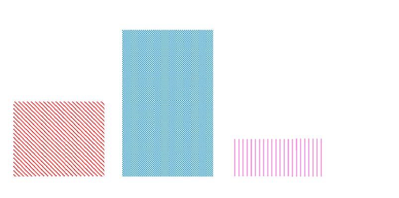
Global Biogeochemical Cycles                                                                        10.1002/2015GB005135

                                         Figure 1. Map showing the Amazon forest study area in gray and the forest monitoring site locations for each property. The
                                         shaded area includes the Amazon River study area and tropical forest areas in the north (Guiana) [Eva et al., 2005]. Each
                                         triangle in the diamond symbol represents one property. Starting with the aboveground biomass in the top right [Malhi
                                         et al., 2006]; woody net primary productivity, in the botton right [Malhi et al., 2004]; change in aboveground biomass, top
                                         left [Baker et al., 2004; Lewis et al., 2004c]; analyzed 2005 drought and pre drought, bottom left [Phillips et al., 2009].

                                         A suite of simulations was performed in order to reproduce the individual and combined effects of climate,
                                         CO2 fertilization, land use, and fire changes on the vegetation (Table 2b). The factorial design of the simula-
                                         tions took into account the following: constant atmospheric CO2 concentration from 1970 (325.7 ppm) and
                                         increasing historical atmospheric CO2 concentration since 1970, simulations with potential vegetation, with
                                         land use change, and with and without fire. We use 1970 as the reference year for switching CO2 on/off for
                                         consistency with the available climate data and because our oldest field observations start in the 1970s, more
                                         specifically in 1971 [Lewis et al., 2004c]. With this set of simulations it was possible to derive the effect of all
                                         factors combined on the vegetation properties (all combined, HistD: current climate, increasing CO2, land use
                                         change, and fire). The individual effect of CO2 fertilization was taken as the difference between two simula-
                                         tions, one applying constant CO2 at 1970 values through the period of analyses (HistE) and another allowing
                                         for increasing CO2 concentrations during our study period (HistB). The individual effect of land use change
                                         was also taken as the difference between two simulations, one with constant land cover (HistA) and another
                                         with historical changes in land cover included (HistD). HistE simulates the effect of climate variability on the

                                                                                   a
Table 2a. Description of Factorial Simulations Performed From 1970 up to 2008
                                                                                                                                                                      b
Simulation           Historical Climate Sheffield 1970–2008                   Atmospheric CO2                        Vegetation                 Natural Disturb Fire

Hist A                              Historical                                  Increasing                     Potential Vegetation                     Fire
Hist B                              Historical                                  Increasing                     Potential Vegetation                     No
Hist C                              Historical                          Constant (1970, 325.7 ppm)             Potential Vegetation                     Fire
Hist D                              Historical                                  Increasing                          Land Use                            Fire
Hist E                              Historical                          Constant (1970, 325.7 ppm)             Potential Vegetation                     No
       c
IBIS_HP                             Historical                                  Increasing                     Potential Vegetation                     No
  a
     All the simulations (HistA to Hist E) starts from the same initial state resulting from a spin up to preindustrial equilibrium up to 1700 and runs forward until
1970 by accounting for historical gradually rising atmospheric CO2 (1700–1970), land use change, natural disturbance (fire), and the recycling 1970–2008
climatology.
   b
     Fire was simulated in all models except for JULES.
   c
     Simulation with modified version of IBIS that includes heterogeneous parameterization across Amazon Basin [Castanho et al., 2013].

CASTANHO ET AL.                                                      CHANGING AMAZON BIOMASS                                                                       21
Global Biogeochemical Cycles 10.1002/2015GB005135
Table 2b. Description of the Individual and Combined vegetation. Because CO2 concentrations in HistE
Effect Studied
were frozen at the 1970 level, this climate analy-
Combined Simulations Analyses sis includes not only the effect of climate but
Hist A Climate and CO2 Fertilization also any lag effect on the biomass of the increas-
Hist B-Hist E CO2 Fertilization ing CO2 prior to 1970. Although this is different
Hist D-Hist A Land Use from the standard in the literature (freezing at
Hist D All Combined
Hist E Climate
preindustrial level, or 280 ppm), we believe this
IBIS_HP Heterogeneous Parameterization experiment setup is best suited to the problem
analyzed here. If we used 280 ppmv as the base-
line, we would simulate the response of the vegetation to climate under a nonrepresentative CO2 concentra-
tion for the period covered by the data (1970–2008).
In order to clarify the role of spatial variation in plant traits a sixth simulation with potential vegetation and
increasing CO2 concentration was included using a newer version of IBIS (called IBIS_HP), which included spa-
tially varying plant traits parameterization [Castanho et al., 2013]. The spatial varying parameterizations
include residence time of carbon in woody biomass, maximum carboxylation capacity of Rubisco (Vmax),
and specific leaf area index. All parameters were derived from RAINFOR network data and were extrapolated
to the entire basin. A detailed description of the methods used is in Castanho et al. [2013].
Natural fire estimates were included in the simulations but the results are not explored in this work because
the contribution to biomass change was very small compared to any other factor.
The analysis focused mainly on the spatial and temporal patterns of aboveground biomass (AGB) and woody
net primary productivity (NPPw) (Table 3). These were explored in two ways: (a) evaluation of model simu-
lated average and spatial gradients of AGB and NPPw across the Amazon study area and (b) examination
of the simulated temporal dynamics of biomass and productivity, here referred to as AGB change (ΔAGB;
or fractional change fΔAGB) and growth rate change (fΔNPPw). In all plot-level data-model comparisons,
an evaluation time period of the models was selected that was identical to the census interval periods from
the field data.
Climatic water stress was quantified using two measures: dry season length (DSL), which is the duration of the
dry season, and maximum cumulative water deficit (MCWD), which is the intensity of the water stress [Malhi
et al., 2009]. DSL is defined based on the number of months with less than 100 mm month1 rainfall in a given
year. The calculation of MCWD involves calculating a water deficit for a given grid cell for a particular month
based on the assumption that evapotranspiration is 100 mm month1. These deficits are then accumulated
over all consecutive months in which precipitation is less than 100 mm to calculate MCWD [Malhi et al., 2009].
2.3. Field Data for Model Comparison
We assembled a wide range of published data from field observations at several sites across the Amazon
study area for evaluation of model results (Figure 1 and Table 3). The sites are all in undisturbed old-growth
forest, with most of them being part of the RAINFOR network (Rede Amazónica de Inventarios Forestales,
Amazon Forest Inventory Network; www.rainfor.org). The RAINFOR project is an international effort to moni-
tor structure, composition, and dynamics of the Amazonian forest in order to better understand their rela-
tionship to soil and climate [Malhi et al., 2002; Peacock et al., 2007]. The RAINFOR field data are plot-level
Table 3. Description of Field Data Used in This Study and the Corresponding References
Property Symbol Computation Units Number of Sites RAINFOR Reference
2
Aboveground biomass AGB kg C m 69 Malhi et al. [2006]
2 1
Net primary woody productivity NPPw kg C m yr 25 Malhi et al. [2004]
2 1
Aboveground biomass change ΔAGB =ΔAGB/Δt kg C m yr 17 Baker et al. [2004]
1
Fractional aboveground biomass change fΔAGB =ΔAGB/AGBo*100 % yr 17 Baker et al. [2004]
1
Growth rate fNPP =NPPw/AGBo*100 % yr 23 Lewis et al. [2004c]
1
Growth rate change ΔfNPP =fNPP2 fNPP1 % yr 23 Lewis et al. [2004c]
2 1
Change in Biomass ΔAGB pre-2005 and 2005 kg C m yr 30 pre-2005 Phillips et al. [2009]
13 2005
CASTANHO ET AL. CHANGING AMAZON BIOMASS 22Global Biogeochemical Cycles 10.1002/2015GB005135
Figure 2. (a) Maximum cumulative water deficit (MCWD) anomaly (mm) for 2005, negative values of MCWD anomaly
represent enhanced water stress and positive values represent reduced water stress; (b) mean MCWD (mm) pre-2005.
Figure 3. Yearly accumulated changes in temperature (temp), dry season length (DSL), and maximum cumulative water
deficit (MCWD) for the time period 1970 to 2008.
CASTANHO ET AL. CHANGING AMAZON BIOMASS 23Global Biogeochemical Cycles 10.1002/2015GB005135
Figure 4. Simulated average (1970–2008) yearly change in aboveground biomass (ΔAGB) for each DGVM (IBIS is in red; ED2 is
in blue; JULES is in magenta) and for each forcing combined (a–c) and individually (d–f). The left axis presents the average
2 1
ΔAGB over the entire study area and time period (kg C m yr ). The right axis presents the time-average ΔAGB integrated
1
over the study area (Pg C yr ). The numbers shown above the bars represent the corresponding values from the right axis.
census data with a general spatial area of one hectare (see references for more detailed information) and
consist of diameter measurements of all individual trees > 10 cm diameter breast high (DBH) within the
inventory plots. Repeated censuses allow diameter growth rates of individual trees to be computed. Tree
mortality and recruitment are also recorded from census to census. Biomass of individual trees is calculated
using the allometric equation of Chave et al. [2005] and summed to give total plot-level biomass of
trees > 10 cm DBH.
Forest plot data were aggregated to 1° spatial resolution (Figure 1 and Table 3) varying from one to six mea-
surement plots in a grid cell, when available. We compiled published values of aboveground live biomass
from 69 grid cells [Malhi et al., 2006]; aboveground woody productivity, 25 gridcells [Malhi et al., 2004];
CASTANHO ET AL. CHANGING AMAZON BIOMASS 24Global Biogeochemical Cycles 10.1002/2015GB005135
Figure 5. Time series of study area-averaged yearly ΔAGB due to climate effect plus lagged effects of the transient pre 1970
CO2 increase, (IBIS is in red, ED2 is in blue, and JULES is in magenta), compared to the maximum cumulative water deficit
(MCWD) anomaly in gray. Shaded areas in red indicate negative anomalies in MCWD (higher water deficit period), while
shaded areas in blue indicate positive anomalies in MCWD (lower water deficit).
changes in aboveground biomass, 17 gridcells [Baker et al., 2004]; and stem growth and mortality rates, 23
sites [Lewis et al., 2004c].
Phillips et al. [2009] analyzed records from long-term plots across Amazonia to assess forest response to the
intense 2005 drought relative to pre-2005 conditions. The authors identified increasing biomass before 2005
and a significant reduction in aboveground biomass due to the 2005 drought. We compared this result to the
model simulations to assess model sensitivity to extreme drought. The precipitation data used in the model
simulations was compared to that used in Phillips et al. [2009] and was found to be similar in spatial distribu-
tion and magnitude. The 2005 drought year showed a clear increase in water stress (MCWD) in the south and
western region of Amazonia (Figure 2a) compared to the average regional water stress, which is concentrated
in the southeastern Amazon (Figure 2b).
2.4. Climate Trends in the Studied Period
Here we briefly analyze the main climate trends from the meteorological data used in this study from
[Sheffield et al., 2006]. There is a decrease in the temperature from 1970 to the mid-70s followed by an
increase until 2008 of about 1°C (Figure 3). This temperature behavior has been identified in other studies
as part of a long-term atmospheric oscillation [Botta et al., 2002; Malhi and Wright, 2004]. Dry season length
(DSL) and maximum cumulative water deficit (MCWD) follow the temperature pattern in the early 70s, with a
decrease in the dry season length and water stress followed by an increase in DSL and water stress to the end
of the record. The interannual variability of the DSL and MCWD is greater than any net trend along the
39 years of this study, as also observed in previous studies [Marengo et al., 2008]. The climatological data ana-
lyses show that except for the first decade (1970–1980), the climate is dominated by interannual variability
and not a strong long-term change.
3. Results
3.1. Amazonian Simulation Results 1970–2008
3.1.1. Carbon Balance (1970–2008)
All models simulate an increase in biomass due to increasing atmospheric CO2 concentrations and climate
variations, and a decrease in biomass due to land use change (Figure 4). However, they differ in magnitude
depending on their sensitivity to each driver of change. ED2 is clearly the most sensitive to climate and the
CO2 fertilization effect, followed by IBIS, then JULES (Figures 4 and 6).
The combined effects of all factors (climate, CO2 fertilization, and land use change) from 1970 to 2008 result
in a simulated AGB gain with IBIS (0.04 PgC yr1) and ED2 (0.17 PgC yr1) and a net loss with JULES (-0.07 PgC
yr-1). This represents an annual increase of about 0.08 and 0.25% (in IBIS and ED2, respectively) and a decrease
of about 0.05% in JULES, in the integrated AGB across the Amazon basin (Figure 4a). In all models land cover
changes impart a decrease in AGB. In IBIS and ED2 the increase in biomass due to climate and CO2 fertilization
CASTANHO ET AL. CHANGING AMAZON BIOMASS 25Global Biogeochemical Cycles 10.1002/2015GB005135
(Figure 4b) more than compensates for the loss of
biomass due to land use change, while the change
simulated by Jules is too small to overcome the
AGB loss from land cover (0.18 in IBIS, 0.17 in
ED2, and 0.21 in JULES PgC yr1, Figure 4f).
Although the land use fraction is prescribed for
all models, the magnitude of the land use effect
differs across models due to differences in
background biomass stocks. The CO2 fertilization
effect is the largest contributor to the simulated
aboveground biomass increase: 0.16 PgC yr1 for
IBIS (77% of change), 0.23 PgC yr1 for ED2 (63%
of change), and 0.10 PgC yr1 for JULES (77% of
change), respectively (Figure 4e) in the last
39 years (1970–2008). Without the CO2
fertilization effect all models would have simu-
lated a net forest biomass loss during the simu-
lation period (Figure 4c). Climate combined to
the lagging effect after freezing CO2 to constant
levels contributed to a small increase in AGB
of 0.05 (IBIS), 0.13 (ED2), and 0.04 (JULES)
PgC yr1 (Figure 4d).
The relative importance of different drivers of
change varies in time and space (Figures 5 and 6).
Although CO2 fertilization exerted the strongest
influence on the C balance in the long term, much
of the interannual variability in C balance was
governed by variability in climate. There was little
evidence of a trend in climate during the simulation
period (Figure 3), but interannual variations were
large and important where changes in biomass
ranged from plus or minus 0.04 kgC m2 yr1
(Figure 5) 3 times larger than the mean annual
climate effect (Figure 4d).
Figure 6. Time series of the fractional aboveground biomass Temporal patterns of ΔAGB were found to be
change accumulated from 1970 to 2008 and averaged over
closely related to patterns of background MCWD
the Amazon study area (a) IBIS, (b) ED2, (c) JULES. Each colored
line represents the individual effect of climate and lagged CO2 (Figure 5). Extreme climate events such as
fertilization effect (blue); CO2 fertilization (green); land use El Niño in 1983 and 1998 and the warm north
change (red); and climate and CO2 fertilization combined tropical Atlantic in 2005 are distinguishable in
(in violet); shaded area represents the maximum net effect the MCWD, and result in simulated biomass
considering CO2 minus the minimum effect not considering
the CO2 fertilization effect. Maps of the fractional accumu- decrease (Figure 5, red shaded areas). More favor-
lated biomass change in 2008 relative to 1970, accounting for able climate periods, particularly during the
(d–f) all forcing, (g–i) climate effect and lagged CO2 fertiliza- 1970s, result in an increase in biomass (Figure 5,
tion effect, (j–l) CO2 fertilization effect only, (m–o) and for land blue areas). Simulated biomass change was
use effect only, for each model, respectively, IBIS, ED2, and
shown to be sensitive to climatic interannual
JULES. Hot colors indicate increase in biomass and cold colors
indicate a decrease in biomass. variability by all models, with higher sensitivity in
ED2 model.
In the first decade (1970–1980) climate changes plus the CO2 lagging effect resulted in a simulated increase
in biomass by all models. ED2 was most sensitive (0.5% yr1 biomass increase), while IBIS and JULES were
about half as sensitive (0.25% yr1 biomass increase) (Figure 6a). After 1980 the climate effect contributed
to a null up to a slight decrease in change in simulated cumulative AGB at the end of the period, in all
models (Figure 6a).
CASTANHO ET AL. CHANGING AMAZON BIOMASS 26Global Biogeochemical Cycles 10.1002/2015GB005135
Figure 6. (continued)
The analysis also revealed interesting temporal (Figures 6a–6c) and spatial patterns (Figures 6d–6o) in biomass
gains/losses. While the CO2 fertilization effect is more apparent in the long term analyses, the climate effect tends
to zero in the long term. The opposite effect is noticed in the short term. This happens because the CO2 fertiliza-
tion effect is a positive and cumulative effect while the climatic effect varies considerably on an inter-annual basis.
Land use change is clearly the most important single-factor driving spatial variability in AGB change in the
studied period of time (Figures 6m–6o), being most pronounced in the southern, southeastern part of the
Amazonian study area. Climate and CO2 effects made modest contributions to the spatial variability
(Figures 6g–6i). There was evidence in our simulations that the strength of the climate and CO2 effects also
varied in different parts of the Amazon. In all models, climate-driven gains in biomass were strongest in the
Table 4. Mean (and Standard Deviation) AGB Stocks and NPPw Across Field Measurement Sites and Corresponding Time Period [Malhi et al., 2006, 2004] and as
Simulated by Each Numerical Model
Field Observation IBIS ED2 JULES IBIS-HP
2
AGB [kg C m ] 14.8(2.7) 11.3(2.3) 11.0(4.2) 14.6(2.0) 13.7(2.3)
2 1
NPPw [kg C m yr ] 0.29(0.07) 0.66(0.06) 0.46(0.22) 0.42(0.20) 0.34(0.04)
CASTANHO ET AL. CHANGING AMAZON BIOMASS 27Global Biogeochemical Cycles 10.1002/2015GB005135
Figure 7. (a) Simulated AGB compared to field estimates from Malhi et al. [2006]; (b) Simulated NPPw compared to field
estimates from Malhi et al. [2004]. The model simulations are IBIS (red), ED2 (blue), JULES (magenta), and IBIS HP (black),
for periods of time and location corresponding to the field measurements.
southwestern edge of the Amazon. ED2 simulated climate-driven declines in biomass in southeastern
Amazon that were not simulated by IBIS or JULES. ED2 and JULES also simulated strong positive CO2 effects
in the southwestern Amazon, in contrast to IBIS, which simulated a weaker response of biomass to CO2 in the
southwestern Amazon than in the remainder of the study area. These results are consistent with a stronger
water use efficiency response under high CO2 over drier regions of the Amazon in JULES and ED2 than in IBIS.
3.2. Forest Plot Data-Model Comparison
3.2.1. Evaluation of Spatial Patterns of AGB and NPPw
Mean simulated aboveground biomass (AGB) values across the study area are within the range of the obser-
vations, while NPPw is systematically overestimated (Table 4). All DGVMs simulated a spatially homogeneous
distribution of biomass and productivity, in contrast to the field observations that show a strong variability
CASTANHO ET AL. CHANGING AMAZON BIOMASS 28Global Biogeochemical Cycles 10.1002/2015GB005135
Figure 8. Fractional AGB change (fΔAGB) simulated by each model compared to fΔAGB from field observations, for periods
of time and location corresponding to the field measurements: IBIS (red), ED2 (blue), JULES (magenta), IBIS_HP (black).
(a) Bar plot representing the average over the corresponding field sites locations; error bars represent the standard
deviation between the sites. (b) Scatter plot comparing simulated to observed estimates by field site.
across the study area (Figure 7). Field data suggest a gradient of lower AGB stock and higher productivity in
western and southern Amazonia and a higher biomass stock and lower productivity in central Amazonia
(AGB ranging from 9 to 20 kg C m2 and productivity ranging from 0.15 to 0.55 kg C m2 yr1) [Malhi et al.,
2006, 2004]. The spatial variability of estimates of AGB and NPPw has been shown by Castanho et al. [2013]
to be strongly related to the spatial heterogeneity of woody residence time and soil fertility, which are
included in IBIS_HP but not in the other models.
The IBIS-HP results, which explicitly include spatially heterogeneous parameterization, are presented for com-
parison (Figure 7, black dots). The IBIS-HP results indicate that consideration of the spatial heterogeneity of
the key model parameters is crucial for capturing the spatial variability of AGB and NPPw observed from field
CASTANHO ET AL. CHANGING AMAZON BIOMASS 29Global Biogeochemical Cycles 10.1002/2015GB005135
Figure 9. Growth rate change (ΔfNPPw) simulated by each model compared to field observations, for periods of time and loca-
tion corresponding to the field measurements: IBIS (red), ED2 (blue), JULES (magenta), IBIS_HP (in black). (a) Bar plot representing
the average over the corresponding field sites, and (b) scatter plot comparing simulated to observed estimates by field site.
data [Castanho et al., 2013]. The average of simulated AGB across the measurement sites is close to that of the
field observations of AGB (13.7(2.3) and 14.8(2.7), IBIS-HP and field observations, respectively) (Table 4). The
NPPw simulated by all models is systematically overestimated compared to the observations. This overesti-
mation is related to the way the models allocate the NPP between the plant compartments, overestimating
the allocation to wood [Castanho et al., 2013]. Correcting for this bias in the IBIS-HP simulation results in a bet-
ter representation of NPPw compared to field estimates (0.34(0.04) versus 0.29(0.07) respectively).
3.2.2. Evaluation of Simulated AGB Change (ΔAGB) and NPPw Change (ΔNPPw) With Forest
Plot-Based Estimates
Estimates based on field data plots show an average ΔAGB of 0.062(0.083) kgC m2 yr1[Baker et al., 2004; Lewis
et al., 2004a, 2004c; Phillips et al., 1998]. The plots in these analyses are located in old growth forests and are not
CASTANHO ET AL. CHANGING AMAZON BIOMASS 30Global Biogeochemical Cycles 10.1002/2015GB005135
Figure 10. Simulated and observed ΔAGB averaged over the sites of analyses. Gray bars represent the pre-2005 period and
black bars represent the 2005 drought period. Gray and black dots show individual site-level data for pre-2005 and 2005 peri-
ods, respectively. (a) Simulated results with the combined effect of Climate and CO2 fertilization effects; (b) Simulated results of
climate effect and lagged pre1970 CO2 increase effects only. Field data observations were adapted from Phillips et al. [2009].
affected by land use change. We compared ΔAGB from field data sites to the simulated values of corresponding
grid cells, accounting for climate and CO2 forcing only (excluding land use change). The mean simulated ΔAGB
was net positive for all models (+0.03 ± 0.01 kg C m2 yr1 for IBIS, +0.017 ± 0.005 kg C m2 yr1 for JULES to +0.04
± 0.01 kg C m2 yr1 for ED2). ED2 simulated the highest mean fΔAGB and was the closest to the mean fΔAGB
across the forest inventory plots (Figure 8a). All three models have very low spatial variability in fΔAGB com-
pared to the field observations (Figure 8b).
Simulated ΔfNPPw varies considerably among the DGVMs and none compare well with the observations
[Lewis et al., 2004a] (Figure 9). Although IBIS_HP simulates AGB and NPPw values that are in better agreement
with the observations than the other models, the simulated fΔAGB and ΔfNPPw is poor (Figure 8, Figure 9).
Thus, none of the models, whether big-leaf or stand-level architecture, capture plot-specific biomass
dynamics. The hypotheses for this response are explored in the discussion section.
3.2.3. Evaluation of Simulated AGB Response to the 2005 Drought
In a manner analogous to the study of Phillips et al. [2009], we compare average annual ΔAGB for observa-
tions (specific field plots) and models before the 2005 drought event to ΔAGB during the 2005 drought year.
Output from simulations considering only CO2 and climate are used for this analysis. Mean-simulated ΔAGB
(Figure 10a, gray bars) pre-2005 is similar to that presented in Figure 4a, for the entire study area. All models
simulate pre-2005 ΔAGB lower or close to observations, despite failing to capture the observed spatial varia-
bility (Figure 10a, gray dots). The field data indicates a decrease in biomass (negative ΔAGB) in most of the
sites in 2005 drought compared to an increase in biomass pre-2005.
CASTANHO ET AL. CHANGING AMAZON BIOMASS 31Global Biogeochemical Cycles 10.1002/2015GB005135
2 1
Figure 11. Aboveground biomass change (kg Cm yr ) pre-2005: of (a) field observations, from model simulation with
2 1
climate only effect (e, b, and f) for IBIS, ED2, and JULES, respectively. Aboveground biomass change (kg Cm yr ) 2005
drought of (c) field observations, form model simulation with climate only effect (g, d, and h) for IBIS, ED2, and JULES,
respectively. (Figures 11a–11d) An overall sink of C (blue) with a positive AGB change in the decadal pre-2005 period.
(Figures 11e–11h) The 2005 drought year with a negative AGB and most of the study area being a source of carbon (red).
Analysis of simulations without increasing CO2 (climate only) shows that despite underestimating ΔAGB
compared to field results, models are able to distinguish between pre-2005 increases in biomass and
decreases in biomass in 2005 due to the drought stress in many sites (Figure 10b). However, the modeled
reduction in ΔAGB due to climate is insufficient to reverse the sign of the change due to CO2 fertilization
and all models suggest that the Amazon continues to be a carbon sink during the 2005 drought
(Figure 10a, black bars).
The spatial distribution of simulated ΔAGB, with climate effect only, in the pre-2005 period in most regions is
a positive (Figures 11a–11d, blue/sink) for all models in qualitative agreement with the observations, but the
models underestimate the magnitude. During the 2005 drought period (Figures 11e–11h, red/source) model
and field data show an overall decrease in biomass with isolated areas of increasing in biomass.
CASTANHO ET AL. CHANGING AMAZON BIOMASS 32Global Biogeochemical Cycles 10.1002/2015GB005135
4. Discussion and Conclusions
4.1. Drivers of Amazon Carbon Balance
This study quantified the importance of the major drivers of variability of the Amazonian carbon balance from
1970 to 2008. Whereas attribution of change is difficult from analysis of the field data alone, models allow for
clear separation of the importance of individual factors. The main factors analyzed were CO2 fertilization,
climate, and land use change.
In undisturbed forest areas, the DGVMs analyzed here agree with forest inventory observations that above ground
biomass has increased across Amazonia over the last years [Baker et al., 2004; Lewis et al., 2004b, 2004c; Phillips
et al., 1998]. Our factorial analysis suggests that the CO2 fertilization effect is the major factor responsible for
the simulated historical increase in AGB (Figure 4e). The climate in the period showed no specific trend resulting
in a close to null contribution in the integrated time; however, it does affect biomass at the interannual scale.
Land use change was shown to be of great importance for the regional carbon budget, being similar in magni-
tude to the CO2 fertilization effect (Figure 4f). In IBIS and ED2, biomass losses due to land use change, although
significant, were insufficient to negate CO2 gains, resulting in an overall gain of biomass over Amazonia over the
simulation period. In the JULES simulations, biomass losses resulting from land use change outweighed biomass
gains due to climate and CO2 fertilization, resulting in a net loss of biomass over Amazonia over the simulation
period. The regional patterns of biomass change closely follow those of deforestation, with biomass decreases
concentrated in the eastern and southern margins of the regions (Figure 6). Areas subject to less deforestation
in central and western Amazonia generally gained biomass. The source of carbon due to deforestation found in
this study (0.18 in IBIS, 0.17 in ED2, 0.21 in JULES PgC yr1, Figure 4f) is well within the estimates in other
works. Aragão et al. [2014] estimate a carbon source due to gross deforestation ranging from 0.12 to
0.23 PgC yr1, simulations with LPJmL resulted in 0.17 to 0.22 PgC yr1 [Poulter et al., 2010].
The magnitude of the biomass changes simulated by the models is broadly in agreement with bottom up stu-
dies, usually based on book-keeping methods. IBIS and ED reported a mean regional sink of 0.04 and
0.17 PgC yr1 (Amazonia-South America Tropical Forest 8 · 106 km2 1970–2008) when all factors were
considered while JULES simulated a net biomass source of 0.07 PgC yr1 over the simulation period
(Figure 4a). Bottom up analyses from Pan et al. [2011], using forest inventory data and long-term ecosystem
C studies, suggested a C sink of 0.07 PgC yr1 (Tropical America, 2000–2007). Malhi [2010] estimated a net sink
of C of 0.03 ± 0.15 PgC yr1 which they concluded was not significantly different from zero (Tropical Americas
8.02 · 106 km2, 2000–2005). Aragão et al. [2014] estimated a current net carbon sink in 2010 for Brazilian
Amazonia on the order of 0.16 PgC yr1 (ranging from sink 0.11 to sink 0.21 PgC yr1); however, the authors
state that this value can be a source in drought years of 0.06 PgC yr1 (ranging from source 0.01 to source
0.31 PgC yr1). The net balance simulated by the models in this study as well as the estimates in literature sug-
gest a null to an average sink of carbon in the Amazon in the last decades. The models also indicate that there is
a significant interannual variability whereby the carbon balance can fluctuate between a sink and a source of
carbon, as well as observed in [Gatti et al., 2014] driven primarily by extreme climate events and the processes
that occur with them. Therefore, future climate, atmospheric CO2 concentration, frequency of extreme climatic
events, as well as the intensity of fires [Balch et al., 2015; Brando et al., 2014], and the rates of deforestation will all
be key factors in determining the contribution of the Amazonian forest to the global C balance.
Our results have clear implications for studies focusing on the future carbon balance of Amazonia. Recent stu-
dies involving simulations of DGVMs with ensembles of climate model forcings have suggested an overall
resilience of Amazonian forests to climate change [e.g., Huntingford et al., 2013; Rammig et al., 2010].
However, such studies generally do not take into account land use change or accurate estimates due to fire.
Persistent future deforestation may effectively cancel or reverse the significant land sink predicted by many
models in the future [Zhang et al., 2015].
Despite the advances made in this study, it is important to acknowledge that the current structure of the
DGVMs used in this study has prevented assessment of some potential mechanisms that may contribute
to Amazonian biomass dynamics [Coe et al., 2013]. In addition to climatic factors (e.g., changing rainfall, tem-
perature, and radiation patterns) and increasing CO2, increasing nutrient deposition, especially nitrogen and
phosphorus, from biomass burning and also long-range transport of Saharan dust, have been considered as
potential agents of dynamic change in Amazonian forests [Lewis et al., 2009]. However, the lack of fully
CASTANHO ET AL. CHANGING AMAZON BIOMASS 33Global Biogeochemical Cycles 10.1002/2015GB005135
interactive nitrogen and phosphorus cycles in the models used in this study precludes assessment of the role
of nutrient deposition on the Amazonian C balance. It has also been proposed that the increasing biomass
storage in Amazonian rainforests reflects recovery from large-scale disturbance events [e.g., Wright, 2005].
However, large disturbances such as blow down events are not really considered in the current simulations.
Finally, an increase in liana abundance over time has been reported in Amazonia [Phillips et al., 2002]. Lianas
are thought to be favored by increasing atmospheric CO2 and can alter forest structure by increasing tree
mortality [Van Der Heijden et al., 2013].
4.2. Sensitivity to Extreme Events
Extreme climatic events play an important role in the global carbon cycle [Reichstein et al., 2013]. Although
the latest evidence suggests that the global land carbon sink continues to increase [Le Quere et al., 2009],
its interannual variability is linked to extreme climatic events. For example, Zscheischler et al. [2014] recently
showed that extreme events, mainly linked to drought, dominate the global interannual variability in gross
primary productivity (GPP). Thus, accurate modeling of the impacts of extreme events is essential for reliable
predictions of climate impacts on global ecosystems.
The Amazon region has experienced a number of extreme drought events in recent decades. These include the
El-Nino–Southern Oscillation (ENSO) events of 1982/1983, 1986/1987, and 1997/1998 as well as the recent
droughts of 2005 and 2010, which were associated with large, positive north Atlantic sea surface temperature
anomalies, with a different spatial fingerprint to ENSO droughts. We found that the three DGVMs evaluated in this
study were unable to reproduce the biomass losses observed in forest inventory data across Amazonia following
the 2005 drought event in Amazonia. This was not an artifact of the forcing climate data, which adequately cap-
tured patterns of rainfall anomalies, but a result of the insensitivity of simulated biomass to drought conditions.
This result is consistent with previous studies that show that models are not able to capture the response of for-
ests to imposed experimental drought, greatly underestimating biomass loss [Galbraith et al., 2010; Powell et al.,
2013; Sakaguchi et al., 2011]. These studies have shown that while simulated carbon fluxes such as gross primary
productivity (GPP) and net primary productivity (NPP) may have large reductions during drought, the effect on
simulated carbon stocks is minimal. The lack of biomass response to drought is likely related to the inadequate
representation of forest carbon turnover and mortality in these models [Galbraith et al., 2013], emphasizing the
need for a revised treatment of drought-induced mortality in DGVMs. As shown by Powell et al. [2013], our ana-
lysis also finds that ED2 is the most sensitive model to drought in terms of its biomass response. Field experiments
of rain exclusion and observations of interannual variability have helped provide a better understanding of the
tropical forest behavior to drought stress. Empirical and mechanistic formulations have been developed to char-
acterize tropical forest tree mortality in response to water stress [Brando et al., 2012; Phillips et al., 2009; Powell
et al., 2013] but have not been incorporated in numerical models yet.
The insensitivity of DGVMs to extreme natural drought events such as the 2005 Amazonian drought event
has significant implications. The study area average simulated carbon fluxes responded to interannual varia-
bility of climate reasonably well (Figure 5). However, the mechanisms involved in the response of vegetation
to interannual variations in temperature and rainfall are fundamentally different to those involved in the
response to extreme events. Responses of vegetation to interannual variation in climate are dominated by
the response of photosynthetic and respiratory fluxes, which DGVMs include. On the other hand, responses
to extreme events, as shown by Phillips et al. [2009] for the 2005 Amazonian drought, are dominated by tree
mortality processes, which these DGVMs do not yet incorporate.
4.3. Spatial Patterns of Stock and Biomass Change
In agreement with previous studies [Delbart et al., 2010], we found that none of models in this study, except
for IBIS_HP as highlighted by Castanho et al. [2013], are able to reproduce observed spatial gradients in bio-
mass and productivity across Amazonia. This stems from a number of model structural deficiencies, including
the lack of interactive cycling of phosphorus, an important determinant of forest structure and productivity in
Amazonia [Quesada et al., 2012] as well as the lack of mechanistic treatment of carbon turnover processes
[Galbraith et al., 2013] and simplistic descriptions of carbon allocation [Malhi et al., 2011].
Increasing CO2 led to increased biomass gains across the entire Amazon region, with relative increases appearing
to be greater in the drier southern region of the Amazon, especially in ED2 and JULES. This may be linked to
increased water use efficiency under higher CO2, an effect that would have greater benefit in drier environments.
Observational data on water use efficiency is rare for tropical forests, but some evidence of increasing water use
CASTANHO ET AL. CHANGING AMAZON BIOMASS 34Table A1. The Canopy Physiological Processes Governing Plant Photosynthesis and How They Control Water and CO2 Fluxes in the Vegetation Canopy for Each of the Numerical Models are
Described in Detail
IBIS ED2 JULES
[Foley et al., 1996; [Medvigy et al., 2009; [Best et al., 2011; Clark et al.,
Kucharik et al., 2000] Moorcroft et al., 2001] 2011; Cox et al., 1998]
CASTANHO ET AL.
[Collatz et al., 1991; C3 photosynthesis is expressed as the minimum of three potential capacities to fix carbon similarly in all models as follows
Farquhar et al., 1980]
2 1
Ag (mol CO2 m s ), Ag ≅ min(Je, Jc, Js)
gross Photosynthesis
rate per unit leaf area
2 1
An (mol CO2 m s ), net An = Ag Rleaf Ao = Ag Rleaf An = (Ag Rleaf)stressf
leaf assimilation rate open stomata
Ac = Rleaf
closed stomata
An = stressfAo + (1 stressf)Ac
2 1
Rleaf (mol CO2 m s ) Rleaf = γVmax
where γ is the leaf respiration cost of Rubisco activity [Collatz et al., 1991]
2 1 C Γ
Je (mol CO2 m s ),
i
Je ¼ αPARl C iþ2Γ
light-limited rate of where a is quantum efficiency, PARl is the photosynthetically active radiation absorbed by the vegetation layer (l ), Ci is the leaf intracellular CO2 concentration and Γ is
photosynthesis the compensation point for gross photosynthesis
2 1 C i Γ
Jc (mol CO2 m s ),
i c 2 o
J c ¼ V max C þK ð1þ ½O =K Þ
Rubisco limited rate of 2 1 1
photosynthesis where Vmax is the maximum capacity of Rubisco (mol CO2 m s ), Kc and Ko (mol mol ) are the Michaelis-Menten parameters for CO2 and oxygen, respectively
p
J Γ
2 1 Vm V max
Global Biogeochemical Cycles
Γ
Js (mol CO2 m s ), Js ¼ 3 8:2 1C þ C -x- Js ¼ 2
i i
photosynthesis is limited V max
by the inadequate rate of Js ¼ 2:2
utilization of triose
phosphate, “sucrose
synthesis limited,”
CHANGING AMAZON BIOMASS
Js = Vmax/2.2
2 1
Ag (mol CO2 m s ), θJ2p Jp ðJe þ J c Þ þ Je Jc ¼ 0 θJ 2p Jp ðJ e þ Jc Þ þ Je Jc ¼ 0
gross Photosynthesis
βA2g Ag Jp þ J s þ J p Js ¼ 0 βA2g Ag Jp þ Js þ Jp Js ¼ 0
rate per unit leaf area
where θ = 0.9 and β = 0.9 are where θ = 0.83 and β = 0.93 are
empirical constants governing empirical constants governing
the sharpness of the transition the sharpness of the transition
between the three potential between the three potential
photosynthesis photosynthesis
1 ½O2 ½O2
Γ (mol mol ) Γ ¼ 2τ Γ ¼ 2τ
compensation point for h i h i
1 1 1 1
gross photosynthesis Γ ¼ 2:3 105 exp 4500 288:15 T Γ ¼ ð21:2 ppmvÞ exp 5000 288:15 T where
0:1ðT 25Þ
τ ¼ 2600 Q10_rs c
where O2 is the atmospheric oxygen concentration where T is ambient temperature
and t is the ratio of kinetic parameter describing with Q10_rs ¼ 0:57:
the partitioning of enzyme activity to carboxylase
or oxygenase function
10.1002/2015GB005135
35Table A1. (continued)
IBIS ED2 JULES
[Foley et al., 1996; [Medvigy et al., 2009; [Best et al., 2011; Clark et al.,
Kucharik et al., 2000] Moorcroft et al., 2001] 2011; Cox et al., 1998]
2 1
Vmax (mol CO2 m s ), The Vmax is an exponential function of temperature The Vmax is an exponential function of temperature The Vmax is an exponential function of temperature
CASTANHO ET AL.
maximum capacity of and it applies a phenomenological cut off for very and it applies a phenomenological cut off for very and it applies a phenomenological cut off for very
Rubisco enzyme low or very high temperatures (278.16 K and low or very high temperatures (To and 318.15 K, low or very high temperatures (Tlow and Tup,
323.16 K, respectively ) (f(Tleaf)). It is also modulated respectively) (f(Tleaf)). It is also ramps down respectively) (f(Tleaf))
by a water stress factor based on plant available photosynthesis in the fall (e(t))
soil moisture (stressf)
Vmax = Vm * f(Tleaf) * stressf
where Vm is prescribed as a function of the PFT Vmax = Vm * f(Tleaf) * e(t) Vmax = Vm * f(Tleaf)
f ðT leaf Þ f ðT leaf Þ f ðT leaf Þ
f(Tleaf), modulate
1 1 1 1 1 1
photosynthesis through exp3500* exp3000 * exp3500*
288:18 T leaf 288:15 T leaf 288:18 T leaf
modifying Vmax by ¼ ¼ ¼
ð1 þ exp 0:4ð278:16 T leaf ÞÞð1 þ expð0:4ðT leaf 323:16ÞÞ ð1 þ exp 0:4ðT o T leaf ÞÞð1 þ expð0:4ðT leaf 318:15ÞÞ 1 þ exp 0:3ðT low T leaf ÞÞð1 þ exp 0:3 T leaf T up Þ
phenomenological as a
function of temperature
ðθθwilt Þ 1
Stressf, modulate 1 expð5Þ stressf ¼
ð1θwilt Þ Demand
photosynthesis by stress stressf ¼ 1 expð5Þ
1þ Supply
factor based on soil
moisture
where θ is the soil moisture content and θ wilt is the where
soil wilting point; the stress factor ranges from 1 Demand ¼ ETmax SLA Bleaf
Global Biogeochemical Cycles
(θ = 1.0) and 0.0 (θ = θ wilt), applied over the Vmax Supply ¼ K w θBroot
1
Modulate photosynthesis eðtÞ ¼ ,
1þðt=t0 Þb
CHANGING AMAZON BIOMASS
through modifying Vmax
in fall where t is the Julian day [Wilson et al., 2000];
parameters t0 and b were obtained from fits to four
key dates derived from MODIS phenology
observations [Zhang et al., 2003]
h i h i
1 1 1 1 1
Kc and Ko (mol mol ), K 1 ¼ 1:5 104 exp 6000 288:15 T K 1 ¼ 1:5 104 exp 6000 288:15 T
Michaelis-Menten h i h i
1 1 1 1
parameters for CO2 and K 2 ¼ 0:25 exp 1500 288:15 T K 2 ¼ 0:836 exp 1400 288:15 T
oxygen, respectively
10.1002/2015GB005135
36You can also read