Asian Development Bank Institute - ADBI Working Paper Series MACROECONOMIC POLICY ADJUSTMENTS DUE TO COVID-19: SCENARIOS TO 2025 WITH A FOCUS ON ASIA
←
→
Page content transcription
If your browser does not render page correctly, please read the page content below
ADBI Working Paper Series

MACROECONOMIC POLICY
ADJUSTMENTS DUE TO COVID-19:
SCENARIOS TO 2025 WITH
A FOCUS ON ASIA

Roshen Fernando and
Warwick J. McKibbin

No. 1219
March 2021

Asian Development Bank Institute
Roshen Fernando is a PhD candidate at the Centre for Applied Macroeconomic Analysis,
 Crawford School of Public Policy, Australian National University, and a research student at
 the ARC Centre of Excellence in Population Ageing Research (CEPAR). Warwick J.
 McKibbin is a professor of public policy and director at the Centre for Applied Macroeconomic
 Analysis, Crawford School of Public Policy, Australian National University; a nonresident
 senior fellow of the Brookings Institution; and director of policy engagement at ARC CEPAR.
 The views expressed in this paper are the views of the author and do not necessarily reflect
 the views or policies of ADBI, ADB, its Board of Directors, or the governments they represent.
 ADBI does not guarantee the accuracy of the data included in this paper and accepts no
 responsibility for any consequences of their use. Terminology used may not necessarily be
 consistent with ADB official terms.
 Working papers are subject to formal revision and correction before they are finalized and
 considered published.

The Working Paper series is a continuation of the formerly named Discussion Paper series; the
numbering of the papers continued without interruption or change. ADBI’s working papers reflect
initial ideas on a topic and are posted online for discussion. Some working papers may develop
into other forms of publication.

The Asian Development Bank refers to “China” as the People’s Republic of China.

Suggested citation:

Fernando, R. and W. J. McKibbin. 2021. Macroeconomic Policy Adjustments due to COVID-19:
Scenarios to 2025 with a Focus on Asia. ADBI Working Paper 1219. Tokyo: Asian Development
Bank Institute. Available: https://www.adb.org/publications/macroeconomic-policy-adjustments-
due-covid-19
Please contact the authors for information about this paper.

Email: Roshen.Fernando@anu.edu.au, Warwick.McKibbin@anu.edu.au

 We thank Shin-ichi Fukuda, John Beirne, and the participants in the Asian Development
 Bank (ADB) meeting for their helpful comments on a draft of this paper. We gratefully
 acknowledge the financial support from the Australian Research Council Centre of
 Excellence in Population Ageing Research (CE170100005). We thank Ausgrid for providing
 electricity use data, which assisted in the calibration of shocks, and Peter Wilcoxen and Larry
 Weifeng Liu for their research collaboration on the G-Cubed model. We also acknowledge
 Jong-Wha Lee’s and Alexandra Sidorenko’s contributions to earlier research on the modeling
 of pandemics.

Asian Development Bank Institute
Kasumigaseki Building, 8th Floor
3-2-5 Kasumigaseki, Chiyoda-ku
Tokyo 100-6008, Japan

Tel:      +81-3-3593-5500
Fax:      +81-3-3593-5571
URL:      www.adbi.org
E-mail:   info@adbi.org

© 2021 Asian Development Bank Institute
ADBI Working Paper 1219                                                 Fernando and McKibbin

Abstract

This paper updates the analysis of the global macroeconomic consequences of the
COVID-19 pandemic in earlier papers by the authors with data as of late October 2020. It
also extends the focus to Asian economies and explores four alternative policy interventions
that are coordinated across all economies. The first three policies relate to fiscal policy: an
increase in transfers to households of an additional 2% of the GDP in 2020; an increase in
government spending on goods and services in all economies of 2% of their GDP in 2020;
and an increase in government infrastructure spending in all economies in 2020. The fourth
policy is a public health intervention similar to the approach of Australia that successfully
manages the virus (flattens the curve) through testing, contact tracing, and isolating infected
people coupled with the rapid deployment of an effective vaccine by mid-2021.

The policy that is most supportive of a global economic recovery is the successfully
implemented public health policy. Each of the fiscal policies assists in the economic recovery
with public sector infrastructure having the most short-term stimulus and longer-term growth
benefits.

Keywords: COVID-19, pandemics, infectious diseases, risk, macroeconomics, DSGE, CGE,
G-Cubed

JEL Classification: C54, C68, F41
ADBI Working Paper 1219                                                                           Fernando and McKibbin

Contents

1.        INTRODUCTION ....................................................................................................... 1

2.        STUDIES ON THE MACROECONOMICS OF COVID-19.......................................... 2

3.        METHODOLOGY ...................................................................................................... 5

          3.1       The G-Cubed Model ...................................................................................... 5
          3.2       Epidemiological Modeling .............................................................................. 7
          3.3       Base Case Scenario and Shocks ................................................................... 9
          3.4       Policy Packages and Additional Shocks....................................................... 21

4.        RESULTS AND DISCUSSION................................................................................. 24

          4.1       Baseline Scenario ........................................................................................ 24
          4.2       Base Case Scenario and Policy Packages................................................... 24
          4.3       Dynamic Results .......................................................................................... 31

5.        CONCLUSION......................................................................................................... 39

REFERENCES ................................................................................................................... 40

APPENDIXES

          1         Infections from the Index Date until 20 October 2020 ................................... 46
          2         Cumulative Infections until 31 December 2020 ............................................ 51
          3         Formulation of Shocks ................................................................................. 56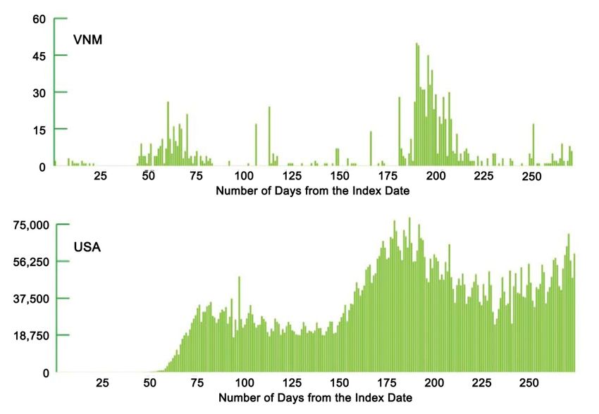
ADBI Working Paper 1219                                                     Fernando and McKibbin

1. INTRODUCTION
The novel coronavirus called SARS-CoV-2 emerged in the People’s Republic of China
(PRC) in late 2019. Amidst increased global interconnectedness, SARS-CoV-2 soon
spread worldwide, leading the World Health Organization (WHO) to recognize the
epidemic as a public health emergency on 30 January 2020 and, subsequently, as the
COVID-19 pandemic on 11 March 2020.
By mid-November 2020, the COVID-19 pandemic had infected over 48 million
individuals and claimed 1.22 million lives. The significant social and economic impacts
have been widespread. Substantial changes have taken place in the behavior of
households and firms in response to the pandemic. Given the highly infectious nature
of the virus, countries worldwide have employed various public health responses,
including lockdowns, isolation of suspected, exposed, and infected individuals, and
contact tracing to track potentially exposed individuals. In addition to the mortality
and morbidity arising from infections, the lockdowns and uncertainty coupled with
diminished confidence have significantly reduced the economic activity in many
economies. The prolonged duration of the pandemic and the scale of policy responses
are likely to have caused the worst economic recession since World War II.
Governments worldwide have implemented a range of economic policy measures in
addition to the health policy responses to curtail the potential economic impacts of
COVID-19. Nevertheless, amidst the uncertainties surrounding the further evolution
of the virus and the timeline for producing and distributing a vaccine globally,
governments have found it challenging to return economic activity to the pre-2020
levels.
McKibbin and Fernando (2020a) circulated a paper on global pandemic scenarios to
policy makers in a range of countries in February 2020 before publicly releasing the
research in March 2020. 1 They used historical experience from other major global
epidemics to explore seven different scenarios for the world economy. They estimated
the epidemiological transmission across countries based on various indicators and
then used the epidemiological outcomes to design a set of economic shocks. They
then applied these shocks to the widely used G-Cubed global economic model. 2 The
analysis gave a range of estimates of the likely macroeconomic consequences of
COVID-19 without public health interventions. McKibbin and Fernando (2020c) updated
the research in June 2020. The second major paper used actual data for the COVID-19
pandemic and then applied these together with assumptions about different durations
of pandemic waves and the health and economic policies that governments had
already announced.
Based on the earlier research, the current paper extends the analysis to a new version
of the G-Cubed model, focusing on Asian economies within a global framework. It also
evaluates plausible policy options to support the economic recovery. We first update
our estimates of the global macroeconomic impact of the pandemic given data up to
November 2020 before considering how the potential policy options could reduce
the adverse macroeconomic consequences of the pandemic. The rest of the paper
proceeds as follows. Section 2 summarizes the estimates of macroeconomic effects
that our previous studies presented and international financial institutions’ forecasts.
Section 3 summarizes the global macroeconomic model and the version used for this
study, the epidemiological modeling approach, the base case scenario and policy

1
    The CEPR also summarized and quickly published this in McKibbin and Fernando (2020b).
2
    See McKibbin and Wilcoxen (1999, 2013) and the discussion below.

                                                  1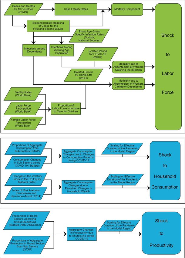
ADBI Working Paper 1219                                          Fernando and McKibbin

packages that we simulate, and the formulation of economic shocks. We then discuss
the pandemic’s macroeconomic consequences and reflect on how the considered
policy options could reduce their severity in Section 4 and present the key conclusions
from our modeling exercise in Section 5.

2. STUDIES ON THE MACROECONOMICS OF COVID-19
In late 2019, when the PRC started reporting infections from a virus similar to SARS-
CoV, the global community expected the outbreaks to confine themselves to the
PRC. This assumption was plausible because the PRC was already experienced in
managing similar outbreaks of coronaviruses and influenza viruses. However, due to
the delay in local officials’ reporting and the strong global connectedness, SARS-CoV-2
soon started spreading into other East Asian countries, the United States, South
Asia, and Europe. By mid-March 2020, countries all around the world had detected
infections.
In early February 2020, the rapid spread of the outbreak caused infectious disease
experts to express concerns about its potential to develop into a pandemic. Policy
makers around the world were still uncertain about the transmissibility or the
contagious nature of the virus and whether its potential health consequences justified
restricting international travel and imposing strict lockdowns at a considerable
economic cost. Requests from policy makers who were familiar with our earlier work
on SARS (Lee and McKibbin 2004a) and Avian influenza (McKibbin and Sidorenko
2006) prompted us to apply and extend the techniques from those studies to explore
the macroeconomic consequences of a potential pandemic resulting from COVID-19.
McKibbin and Fernando’s (2020a, b) research, released in early March 2020,
evaluated seven possible scenarios.
The first three scenarios assumed that the outbreak would predominantly affect the
PRC, with different attack rates, but would remain in the PRC with some spillover due
to global risk assessment changes. The next three scenarios evaluated a pandemic—a
virus transmitted to all countries—with varying attack rates. The seventh scenario
focused on a mild yet recurring pandemic. Since the epidemiological and virological
information about the virus was minimal in February 2020, we utilized the past global
experiences of global influenza outbreaks to derive the potential attack rates.
Table 1 summarizes the assumptions underlying the scenarios in McKibbin and
Fernando (2020a, b). We introduced shocks to mortality, morbidity, productivity by
sector, consumption, government expenditure, and equity risk premia. The last four
scenarios used the experience in the PRC as a benchmark for the shocks. We
adjusted these with an index of vulnerability that we developed to scale the shocks
across the other countries. The simulations provided a range of estimates about the
potential economic consequences of pandemics with varying degrees of severity. The
results clearly showed the economic and financial costs of not containing the public
health emergency.

                                          2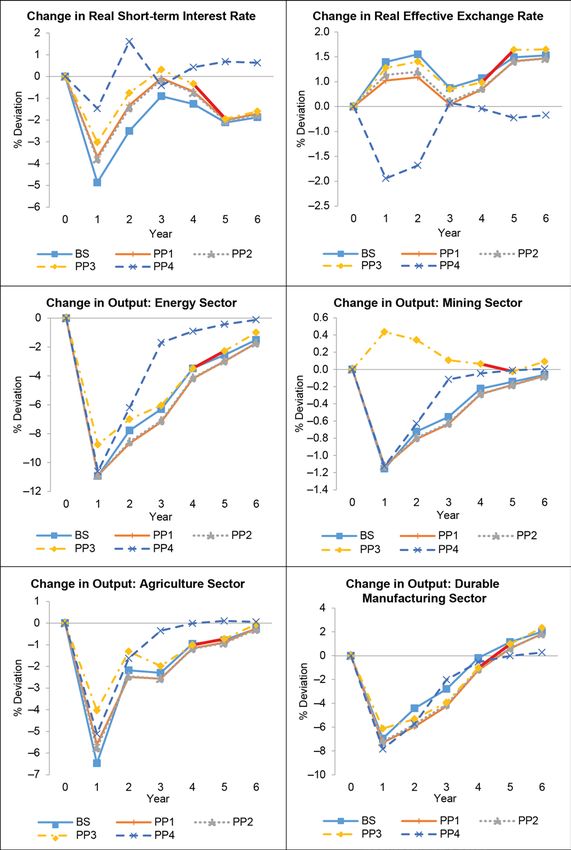
ADBI Working Paper 1219                                                         Fernando and McKibbin

       Table 1: Scenario Assumptions in The Global Macroeconomic Impacts
                          of COVID-19: Seven Scenarios
                                                                                  Shocks      Shocks
                                          Attack        Case                     Activated   Activated
             Countries                    Rate in   Fatality Rate   Nature of                 Other
Scenario     Affected      Severity      the PRC     in the PRC      Shocks         PRC      Countries
1               PRC         Low           1.0%           2.0%       Temporary        All       Risk
2               PRC        Medium        10.0%           2.5%       Temporary        All       Risk
3               PRC         High         30.0%           3.0%       Temporary        All       Risk
4              Global       Low          10.0%           2.0%       Temporary        All        All
5              Global      Medium        20.0%           2.5%       Temporary        All        All
6              Global       High         30.0%           3.0%       Temporary        All        All
7              Global       Low          10.0%           2.0%       Permanent        All        All
Source: McKibbin and Fernando (2020a).

With the gradual evolution of the COVID-19 pandemic, more information has become
available, especially regarding the cases, deaths, and government policy responses.
The health policy responses mainly focused on raising awareness, encouraging
behavioral changes and respiratory hygiene, and elevating health systems’ capacity for
testing, contact tracing, isolating, quarantining, and treating infected individuals amidst
the absence of a vaccine. Many countries imposed movement restrictions and enforced
lockdowns until a vaccine would become available. However, as the movement
restrictions and lockdowns came at a high economic cost, many countries were
reluctant to implement or to sustain these policies for an extended period. In the
absence of significant movement restrictions and lockdowns, the infections and deaths
surged. While countries experimented with the trade-offs of various strategies in real
time, people lost their lives and the economic costs continued to soar. By June 2020,
we had enough information to simulate the pandemic’s six plausible scenarios to inform
policy makers about the macroeconomic consequences of a prolonged pandemic.
By July 2020, in addition to the global economic forecasts that international financial
institutions had produced, only a few studies were attempting to model the global
macroeconomic consequences of COVID-19. The studies by Maliszewska, Mattoo,
and van der Mensbrugghe (2020), the World Bank (2020a), and the World Trade
Organization (2020) utilized computable general equilibrium (CGE) models and mainly
focused on the impact of mortality, morbidity, and increased production costs on the
economies. A study by the IMF (2020a), which utilized a semi-structural dynamic
stochastic general equilibrium (DSGE) model, also included disruptions to financial
markets.
In June 2020, we had data on the pandemic that could inform our scenarios’ design, so
we updated our original study (McKibbin and Fernando 2020c). Table 2 summarizes
these scenarios. These differed in the intervals of surges and whether economies
responded with or without lockdowns. One of the alternative scenarios consisted of
24 simulations in which we assumed that a given country responded well to the
pandemic. In contrast, all the other countries were unsuccessful and experienced high
economic costs.
We imposed a range of shocks to the labor supply due to changes in mortality and
morbidity, shocks to productivity (capturing changes in the cost of doing business,
shocks to consumption, shocks to equity risk premia for sectors, which affected
investment), and shocks to country risk premia. We also imposed shocks to
government expenditure from stimulus packages, distinguishing between government

                                                     3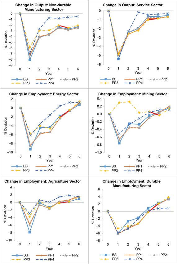
ADBI Working Paper 1219                                                   Fernando and McKibbin

spending, household transfers, and wage subsidies. We simulated these shocks in
the G-Cubed modeling framework (as Section 3.1 describes), which combines the
strengths of the CGE and DSGE modeling approaches. The study produced a
comprehensive set of results for various macroeconomic variables, including real GDP,
private investment, consumption, trade balance, employment, interest rates, inflation,
and exchange rates. The results reinforced the argument that the key to alleviating the
adverse economic consequences was to restore the confidence among economic
agents. As rational households would avoid catching the infection, regardless of
lockdowns, controlling the pandemic when there is a surge in cases and the risk
of transmission is high is central to maintaining economic activities. The approaches
to formulating the shocks and the results of the paper are available from
https://cama.crawford.anu.edu.au/covid-19-macroeconomic-modelling-results-
dashboard.

        Table 2: Scenario Assumptions in Global Macroeconomic Scenarios
                            of the COVID-19 Pandemic
                     Number of Waves and                  Number of Waves and
                      Lockdowns in 2020                    Lockdowns in 2021
                  Number of         Existence of       Number of      Existence of   Recurrence
Scenario           Waves            Lockdowns           Waves         Lockdowns       after 2021
1                      1                 Yes               1              Yes           No
2                      1                 Yes               1              Yes           Yes
3                      2                 Yes               1              Yes           No
4                      2                 Yes               2              Yes           No
5                      1                 Yes               1              No            Yes
                       1                 No
6                 Country of             Yes           Country of          -             No
                  Interest—1                           Interest—0
                  Rest of the            Yes           Rest of the        Yes            No
                   World—2                              World—2
Source: McKibbin and Fernando (2020c).

Some of the economic forecasts that the international financial institutions released,
contemporary to McKibbin and Fernando (2020c), have recently undergone revision.
Table 3 summarizes the economic forecasts relevant to the countries and regions on
which the current paper focuses. We obtained the estimates from the Global Economic
Prospects Report (World Bank Group 2020), World Economic Outlook (IMF 2020a),
Asian Development Outlook (Asian Development Bank [ADB] 2020), and Global
Economic Outlook (Organisation for Economic Co-operation and Development [OECD]
2020). If forecasts for a particular country were not explicitly available, we used the
country’s economic forecast for the region to which it belongs.
All of the global studies show that COVID-19 is likely to have created a global
recession that could be as severe as the one that occurred after World War II. While a
critical determinant of the scale of the global economic consequences of COVID-19 will
be the timing and availability of an effective vaccine, a vaccine alone is unlikely to
generate a rapid path to recovery. Thus, the economic debates now focus more on
policies to support this recovery. Even though a range of policy options is apparent in
the literature, studies have not yet evaluated the potential economic trade-offs of
various policy options widely at the global level. McKibbin and Vines (2020) assessed
the importance of international cooperation in driving the recovery and how it could
improve the global economic outcomes. We extend this contribution, in this paper, by

                                                   4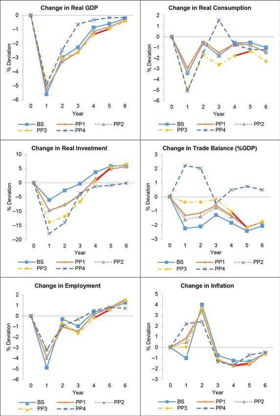
ADBI Working Paper 1219                                              Fernando and McKibbin

evaluating the potential of a range of fiscal policy options that governments across the
world could adopt to support the recovery.

Table 3: Summary of Economic Forecasts by International Financial Institutions
              World Bank Group
Source             (2020)           IMF (2020a)         ADB (2020)          OECD (2020)
              % Change in Real   % Change in Real
               GDP from the       GDP from the       GDP Growth Rate      Projected Change
Description    Previous Year      Previous Year       (% per annum)            in GDP
                                                                           2020       2020
                                                                          (Single   (Double
Year           2020       2021    2020      2021      2020      2021        Hit)      Hit)
AFR           –2.80       3.10    –3.00     3.10      NA         NA        NA         NA
AUS           –7.00       3.90    –5.80     3.90      NA         NA       –5.00      –6.30
CHN            1.00       6.90     1.90     8.20      1.80      7.70      –2.60      –3.70
EUW           –9.10       4.50    –8.30     5.20      NA         NA       –9.10     –11.50
IND           –3.20       3.10   –10.30     8.80     –9.00      8.00      –3.70      –7.30
INO            0.00       4.80    –3.40     6.20     –1.00      5.30      –2.80      –3.90
JPN           –6.10       2.50    –5.30     2.30      NA         NA       –6.00      –7.30
KOR           –7.00       3.90    –5.80     3.90     –1.00      3.30      –1.20      –2.00
LAM           –7.20       2.80    –8.10     3.60      NA         NA        NA         NA
MEN           –4.20       2.30    –4.10     3.00      NA         NA        NA         NA
MYS           –3.10       6.90    –3.40     6.20     –5.00      6.50       NA         NA
OAS           –2.70       2.80    –1.70     8.00     –6.80      7.10       NA         NA
OEC           –7.00       3.90    –7.10     5.20      NA         NA       –8.45      –9.7
PHL           –1.90       6.20    –3.40     6.20     –7.30      6.50       NA         NA
ROW           –2.40       4.70    –4.10     3.00     –2.10      3.90       NA         NA
THA           –5.00       4.10    –3.40     6.20     –8.00      4.50       NA         NA
US            –6.10       4.00    –4.30     3.10      NA         NA       –7.30      –8.50
VNM            2.80       6.80    –3.40     6.20      1.80      6.30       NA         NA

3. METHODOLOGY
3.1 The G-Cubed Model
This paper applies a global intertemporal general equilibrium model with
heterogeneous agents called the G-Cubed multi-country model. This model is a hybrid
of the dynamic stochastic general equilibrium (DSGE) models and computable general
equilibrium (CGE) models that McKibbin and Sachs (1991) and McKibbin and Wilcoxen
(1999, 2013) developed.
The version of the G-Cubed (M) model that we use in this paper is from the study by
Liu and McKibbin (2020), who extended the original model that McKibbin and Wilcoxen
(1999, 2013) documented. Version 6M of the model consists of six sectors, eleven
countries, and seven regions. Table 4 presents all the regions and sectors in the
model. Some of the data inputs include the I/O tables from the Global Trade Analysis
Project (GTAP) database (Aguiar et al. 2019), enabling us to differentiate sectors by
country of production within a DSGE framework. Firms in each sector in each country
produce output using the primary factor inputs of capital (K) and labor (L) as well as the

                                            5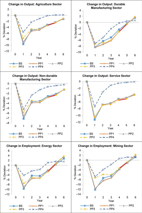
ADBI Working Paper 1219                                                       Fernando and McKibbin

intermediate or production chains of inputs in energy (E) and materials (M). These
linkages apply both within a country and across countries.
McKibbin and Wilcoxen (1999, 2013) documented the approach that the G-Cubed
model embodies. Several key features of the standard G-Cubed model are worth
highlighting here.
First, the model accounts for stocks and flows of physical and financial assets. For
example, budget deficits accumulate into government debt, and current account deficits
accumulate into foreign debt. The model imposes an intertemporal budget constraint
on all households, firms, governments, and countries. Thus, long-run stock equilibrium
arises through the adjustment of asset prices, such as the interest rate for government
fiscal positions or real exchange rates for the balance of payments. However, the
adjustment toward each economy’s long-run equilibrium can be slow, occurring over
much of a century.
Second, in G-Cubed, firms and households must use money that central banks issue
for all transactions. Thus, central banks in the model set short-term nominal interest
rates to target macroeconomic outcomes (such as inflation, unemployment, exchange
rates, etc.) based on the Henderson–McKibbin–Taylor monetary rules (Henderson and
McKibbin 1993; Taylor 1993). These rules aim to approximate the actual monetary
regimes in each country or region in the model. They tie down the long-run inflation
rates in each country and allow short-term policy adjustments to smooth fluctuations in
the real economy.

                      Table 4: Overview of the G-Cubed (M) Model
Countries (11)                        Sectors (6)
Australia (AUS)                       Energy
PRC (CHI)                             Mining
India (IND)                           Agriculture (including fishing and hunting)
Indonesia (INO)                       Durable manufacturing
Japan (JPN)                           Non-durable manufacturing
Republic of Korea (KOR)               Services
Malaysia (MYS)
Philippines (PHL)                     Economic Agents in each Country (3)
Thailand (THA)                        A representative household
United States (US)                    A representative firm (in each of the six production sectors)
Viet Nam (VNM)                        The government
Regions (7)
Latin America (LAM)
Middle East and North Africa (MENA)
Other Asia (mainly South Asia excluding India) (OAS)
Rest of the Advanced Economies (Canada and New Zealand) (OEC)
Rest of the World (mainly Eastern Europe and Central Asia) (ROW)
Sub-Saharan Africa (AFR)
Western Europe (EUW)

Third, nominal wages are sticky and adjust over time based on country-specific labor
contracting assumptions. Firms hire labor in each sector up to the point at which the
marginal product of labor equals the real wage, which we define in terms of that
sector’s output price level. Any excess labor enters the unemployed pool of workers.
Unemployment or the presence of an excess demand for labor causes the nominal

                                                 6
ADBI Working Paper 1219 Fernando and McKibbin
wage to adjust to clear the labor market in the long run. In the short run, unemployment
can arise due to structural supply shocks or aggregate demand changes in the
economy.
Fourth, rigidities prevent the economy from moving quickly from one equilibrium to
another. These rigidities include the nominal stickiness that wage rigidities cause and
firms’ costs of adjustment in investment, with physical capital being sector specific in
the short run. A lack of complete foresight in the formation of expectations and among
monetary and fiscal authorities following particular monetary and fiscal rules also
affects the adjustment path. Short-term adjustments to economic shocks can be very
different from long-run equilibrium outcomes. A focus on short-run rigidities is essential
for assessing the impact over the first decades of a major shock.
Fifth, we incorporate heterogeneous households and firms. We model firms separately
within each sector. We assume two types of consumers in each economy and two
types of firms within each sector within each country. One group of consumers and
firms bases its decisions on forward-looking expectations. The other group follows
simple rules of thumb that are optimal in the long run.
3.2 Epidemiological Modeling
Although the virus outbreak started in late 2019 in the PRC, it reached other parts
of the world at different times. Some countries experienced the pandemic early and
appeared to have controlled the first waves. Some other countries have also
experienced second waves. Overall, the pandemic is continuing in a majority of
countries. For each country, we model the likely number of infections and deaths due
to COVID-19 for 2020 by using actual data up to late October 2020 and then project
the remainder of 2020 and subsequent years.
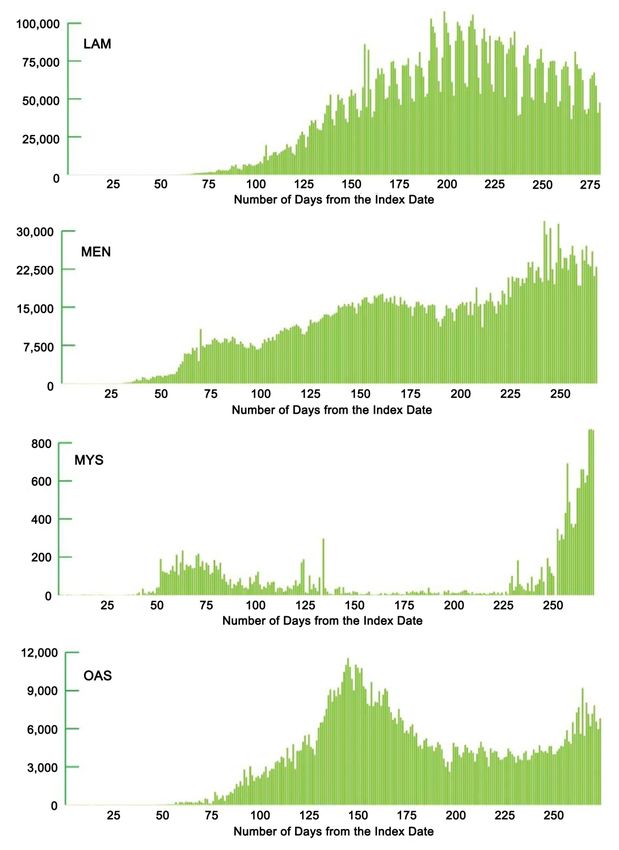
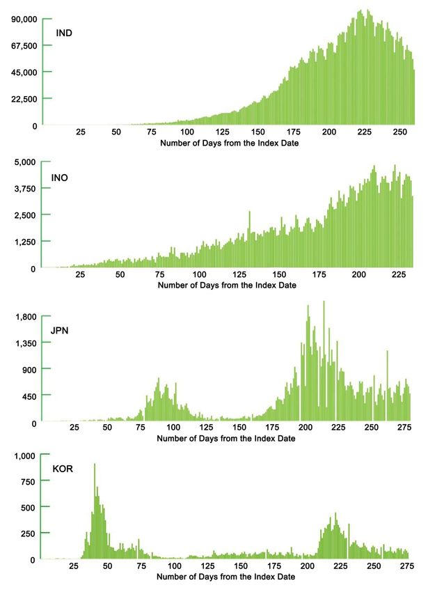
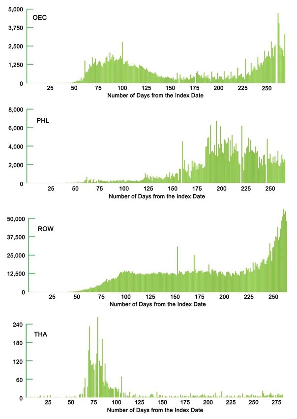
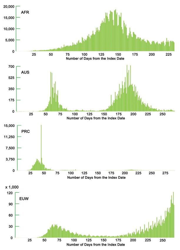
To determine whether the first wave is continuing or has ended for a particular country
or region, we analyze the daily cases via Our World in Data (2020) from late 2019 to
20 October 2020. We aggregate the infection numbers by the countries and regions in
the model and visually approximate whether the first wave is continuing or has ended.
If there is more than one significantly observable wave, which is clearly distinguishable
from surges or spikes, we estimate the likely day on which the first wave could have
ended. Here, we check for a considerable interval between the waves with zero or
very few new cases for countries. For regions, we check for the global minimum among
the inflection points. Appendix 1 presents the infections in each model region up to 20
October 2020. Table 5 summarizes the index date for the model regions, the status of
the first wave as of 20 October 2020, and the duration of the first and second waves (in
the case that a second wave has emerged).
Based on the pandemic status, whether the first or the second wave is continuing, we
estimate the cumulative curve for cases using a non-linear logistic approximation from
20 October 2020 to 31 December 2020. The logistic approximation assumes that the
momentum that the pandemic demonstrated up to 20 October 2020 would continue.
Due to this assumption, the total number of cases does not reflect the later emergence
of new clusters of cases. Table 6 summarizes the infections during the first and second
(if applicable) waves for the model regions until 31 December 2020. Appendix 2
presents the cumulative curves for cases for the current wave for the model regions.
7ADBI Working Paper 1219 Fernando and McKibbin
Table 5: Status of the Pandemic Waves in the Model Regions
Duration of the First Wave Duration of the
Status of the (if the First Wave has Second Wave
Model Index Date for the First Wave as of Ended or as of as of
Region First Wave 20 October 2020 31 December 2020) (Days) 31 December 2020
AFR 28 February 2020 Continuing 307
AUS 25 January 2020 Ended 119 222
CHN 31 December 2019 Continuing 366
EUW 25 January 2020 Ended 163 178
IND 30 January 2020 Continuing 336
INO 2 March 2020 Continuing 304
JPN 15 January 2020 Ended 135 216
KOR 20 January 2020 Ended 108 238
LAM 14 January 2020 Continuing 352
MEN 27 January 2020 Continuing 339
MYS 25 January 2020 Ended 160 181
OAS 21 January 2020 Continuing 345
OEC 26 January 2020 Ended 159 181
PHL 30 January 2020 Continuing 336
ROW 1 February 2020 Continuing 334
THA 13 January 2020 Continuing 353
US 21 January 2020 Continuing 345
VNM 24 January 2020 Ended 101 241
Table 6: Total Infections in the Model Regions
Infections during the Infections during the
Model Region First Wave Second Wave Total Infections
AFR 1,241,929 - 1,241,929
AUS 7,081 20,328 27,409
CHN 91,006 - 91,006
EUW 1,490,568 9,420,611 10,911,179
IND 9,335,908 - 9,335,908
INO 603,454 - 603,454
JPN 16,651 78,015 94,666
KOR 10,806 16,436 27,242
LAM 11,558,520 - 11,558,520
MEN 3,702,391 - 3,702,391
MYS 8,640 194,491 203,131
OAS 1,024,012 - 1,024,012
OEC 105,373 374,124 479,497
PHL 401,533 - 401,533
ROW 3,559,084 - 3,559,084
THA 3,700 - 3,700
US 9,332,319 - 9,332,319
VNM 270 870 1,140
8ADBI Working Paper 1219 Fernando and McKibbin
3.3 Base Case Scenario and Shocks
We first solve the model without a pandemic occurring in 2020. We then create a base
case scenario that is our best guess about the pandemic’s current state. In the base
case scenario, we introduce the pandemic shocks to estimate the macroeconomic
consequences in 2020 due to disruptions to economic activities emanating from
COVID-19-related health effects, behavioral changes of households and firms, and
government policy responses. In this base case, we assume that there is no available
vaccine yet and that complete elimination of SARS-nCoV-2 might be ambitious
(Heywood and Macintyre 2020). We assume that the pandemic will then recur at a
declining rate over future years, causing all the shocks to decline at the same rate.
Below, we discuss the shocks that we developed in the base case scenario.
Appendix 3 contains flowcharts that present a schematic view of the construction of the
shocks. Further details are also available on the results dashboard accessible via:
https://cama.crawford.anu.edu.au/cama-publications/asian-development-bank-institute-
modelling-results-dashboard.
3.3.1 Shock to the Labor Supply
The shock to the labor supply originates from the mortality and morbidity related to the
infection. When formulating the mortality shock, we first obtain the COVID-19 case
fatality rates for the model regions as of 20 October 2020 and apply those rates to the
total infections that we find from the epidemiological modeling, as Section 3.2 explains.
We then compute the deaths as a percentage of the total population to estimate the
epidemiological shock’s magnitude. As deaths would mean a loss of the existing and
potential labor force for an economy, the shock applies permanently in the simulations.
Table 7 presents the case fatality rates, the estimated number of deaths in 2020, and
the magnitude of the mortality shock in 2020.
The morbidity shock has two elements. Firstly, members of the labor force cannot work
if they catch or are exposed to the infection. Therefore, we assume that a proportion of
the labor force would not work for the standard isolation or quarantine period, following
the recommendation of the WHO, of 14 days. To estimate the proportion of the labor
force, within the age group of 20–59 years, infected or exposed to the infection, we use
the reports from the medical authorities of the countries (see Australian Government
Department of Health 2020; California Department of Public Health 2020; Cam 2020)
and the age breakdown of infections from Statista (2020a–j). For the model regions for
which this information is not available, we approximate it using a country or region that
closely reflects its epidemiological characteristics. Using the proportion of the labor
force affected and the World Bank (2020b) data on the labor force participation in the
model regions, we calculate the number of productive days lost and obtain the
proportion of days lost in a 251-day working year.
Secondly, we assume that a proportion of the labor force, equal to 70% of its female
labor force participation, would lose productive time due to caregiving for dependent
children in the 0–19 years age group who catch the infection. Assuming the same
isolation or quarantine period of 14 days and using the World Bank (2020c) data on
female labor force participation rates, we estimate the proportion of days lost due to
caregiving in a 251-day working year. As children have been less vulnerable to the
infection, the second component of the morbidity shock is smaller than the first. Table 8
presents the magnitudes of the morbidity shocks.
9ADBI Working Paper 1219 Fernando and McKibbin
Table 7: Case Fatality Rates, Deaths in 2020, and Mortality Shock in 2020
Model Region Case Fatality Rate Deaths in 2020 Mortality Shock in 2020
AFR 2.13% 26,444 0.0023%
AUS 3.30% 905 0.0036%
CHN 5.21% 4,739 0.0003%
EUW 2.57% 280,301 0.0645%
IND 1.52% 141,564 0.0103%
INO 3.45% 20,846 0.0076%
JPN 1.79% 1,697 0.0013%
KOR 1.76% 481 0.0009%
LAM 2.31% 266,843 0.0408%
MEN 3.16% 117,009 0.0214%
MYS 0.89% 1,807 0.0056%
OAS 0.95% 9,687 0.0016%
OEC 3.24% 15,553 0.0365%
PHL 1.86% 7,462 0.0068%
ROW 2.08% 73,889 0.0177%
THA 1.59% 59 0.0001%
US 2.68% 250,081 0.0756%
VNM 3.07% 35 0.0000%
Table 8: Components of the Morbidity Shock in 2020
(Lost Days as a Proportion of Total Working Days)
Model Region Absenteeism due to Infection Absenteeism due to Caregiving
AFR 0.0070% 0.0003%
AUS 0.0073% 0.0073%
CHN 0.0004% 0.0001%
EUW 0.1540% 0.0816%
IND 0.0339% 0.0050%
INO 0.0109% 0.0006%
JPN 0.0061% 0.0035%
KOR 0.0034% 0.0019%
LAM 0.0880% 0.0048%
MEN 0.0342% 0.0042%
MYS 0.0428% 0.0222%
OAS 0.0129% 0.0062%
OEC 0.0754% 0.0713%
PHL 0.0234% 0.0023%
ROW 0.0430% 0.0025%
THA 0.0004% 0.0001%
US 0.2213% 0.1617%
VNM 0.0001% 0.0000%
3.3.2 Shock to Total Factor Productivity
The productivity shock results from the lockdowns that governments have imposed to
reduce the transmission of the virus. We estimate the shock to productivity for each
sector in each country using the durations of the lockdowns and the proportion of broad
production sectors that the lockdowns disrupted.
10ADBI Working Paper 1219 Fernando and McKibbin
When calculating the duration of the lockdowns, we use the data on workplace closure
across the world from the Coronavirus Government Response Tracker (Blavatnik
School of Government 2020). The database reports the workplace closures at three
levels of stringency; at the third level, only essential workplaces, such as grocery stores
and pharmacies, operate. Thus, different days have different stringency levels. To
calculate the overall stringency level, we allocate a weight of 33.33% to days with
stringency of level 1, 66.66% to days with stringency of level 2; and 100% to days with
stringency of level 3. Weighting different stringency levels enables us to calculate an
effective number of days when stringency of level 3 would have prevailed. We further
split the number of days of workplace closures into two waves for 187 countries and
calculate the number of days with effective workplace closures as a proportion of the
total duration of the pandemic. By using the pandemic’s duration, which we derive from
the epidemiological modeling, we calculate the effective number of months with
workplace closures except for essential production sectors.
When determining the proportions of sectors that do not operate during lockdowns, we
utilize the estimates from the Australian Bureau of Statistics (Australian Broadcasting
Cooperation [ABC] 2020) and AUSGRID for Australia and from Statista (2020k–m) for
Australia, the UK, and India. We then multiply the sub-sectors’ output shares in the
broad sectors by the proportions of sectors not operating to obtain the ratios of broad
sectors not operating. This calculation allows us to differentiate the proportions of
broad sectors not operating across the model regions even though we assume similar
behavior in sub-sectors across the world in this regard. Finally, we scale the
proportions depending on the lockdown duration (as a proportion of a year) to obtain
the productivity shocks for broad sectors.
Table 9 summarizes the effective durations of lockdowns in months in 2020 for the
model regions. Figure 1 presents the proportions of broad sectors not operating in the
model regions.
Table 9: Effective Lockdown Duration
(Months)
Model Region Lockdown Duration (Months)
AFR 6
AUS 4
CHN 5
EUW 5
IND 5
INO 6
JPN 4
KOR 6
LAM 5
MEN 6
MYS 6
OAS 6
OEC 4
PHL 6
ROW 4
THA 4
US 4
VNM 5
11ADBI Working Paper 1219 Fernando and McKibbin
Figure 1: Proportions of Sectors Not Operating during the Pandemic in 2020
3.3.3 Shock to Consumption
As Section 3.1 describes, households maximize their lifelong utility from consumption.
In achieving this objective, changes in household consumption during the pandemic
would arise due to a variety of factors, including changes in income from employment,
changes in the value of future wealth due to the long-term implications of the current
impacts from the pandemic, changes in the relative prices in different sectors, changes
in interest rates, changes in the ability to consume certain goods and services, as well
as changes in consumer preferences. While some of these effects are endogenous to
the model, the consumer preferences in each broad sector and the risk premium on the
discount rate that households use to discount their future income to calculate human
wealth are exogenous to the model.
Using the data from consumer surveys that Statista (2020n) conducted in Australia,
we map the changes in consumer preferences in various activities onto production
sub-sectors. We then aggregate the changes in consumer preferences to the broad
sectors across the model regions using the consumption shares that sub-sectors
claim within aggregated sectors. Similar to the productivity shock that Section 3.3.2
discussed, the aggregation of consumer preference changes in the sub-sectors to the
broad sectors allows us to vary the overall consumption in the aggregate sectors
despite assuming similar consumption changes for sub-sectors. Then, we adjust the
changes in consumer preferences in broad sectors by the duration of the pandemic.
We estimate the exogenous shock to the aggregate consumption in the model regions
by aggregating the sector consumption changes using the overall sector consumption
shares in the overall consumption. Figure 2 presents the changes in consumer
preferences in the model regions by broad sectors. Table 10 shows the changes
in overall consumption in the model regions that we aggregate from the sectoral
preference shifts.
12ADBI Working Paper 1219 Fernando and McKibbin
Figure 2: Changes in Consumption Preferences during the Pandemic
Table 10: Exogenous Shocks to Aggregate Consumption
from Preference Shifts in 2020
Changes in Overall Consumption
Model Region Changes in Overall Consumption as a Proportion of the GDP
AFR –8.33% –2.04%
AUS –11.90% –2.19%
CHN –15.18% –1.50%
EUW –11.39% –2.18%
IND –9.29% –1.79%
INO –11.30% –2.17%
JPN –4.67% –0.90%
KOR –14.53% –2.10%
LAM –11.00% –2.52%
MEN –12.38% –2.39%
MYS –12.19% –1.61%
OAS –13.22% –2.26%
OEC –9.12% –1.82%
PHL –11.74% –3.12%
ROW –8.17% –1.53%
THA –8.53% –1.31%
US –12.03% –2.94%
VNM –7.67% –1.70%
We model the second impact on consumption as a change in the risk premia that
households use to discount their future labor income to calculate their human wealth.
We approximate the changes in risk premia by using the movement of the US VIX
(volatility) Index (Wall Street Journal (WSJ) 2020a), which gives a measure of the
change in market sentiment. We approximate the volatility in the US VIX from March to
October 2020 and take its deviation from the volatility during the same period in 2019.
We then approximate the changes in risk premia in other model regions using the Risk
Aversion Index that Gandelman and Hernández-Murillo (2014) developed. For model
13ADBI Working Paper 1219 Fernando and McKibbin
regions for which the index is not available, we approximate it using their closest peers
in respect of their economic characteristics. We then obtain the shock to risk premia by
scaling the changes in risk premia by the effective durations of lockdowns. Figure 3
presents the values of the Index of Risk Aversion for the model regions in comparison
with the US. Figure 4 shows the magnitude of the shock to risk premia in the model
regions in 2020.
Figure 3: Index of Risk Aversion (US = 100)
Figure 4: Shock to Risk Premia in the Discount Rate for Human Wealth in 2020
3.3.4 Shocks to Country and Sector Risk Premia
While all countries have responded to the pandemic, the actual policy responses have
differed across countries. Financial markets have reflected these differences when
investors have rebalanced their portfolios to diversify the risks. We map these changes
14ADBI Working Paper 1219 Fernando and McKibbin
in relative risks in different countries and sectors to shocks for the model using country
and sector risk premium shocks.
When constructing the shock to country risk premia, we follow the approach that Lee
and McKibbin (2004a, b) and McKibbin and Sidorenko (2006, 2009) introduced and
McKibbin and Fernando (2020a, b, c) improved. The approach involves constructing
three indices for health, governance, and financial risks.
The Index of Health Risk is the average of the Index of Health Expenditure per capita,
which we construct using the health expenditure per capita data from the World Health
Organization (WHO) (2019). We create the Index of Health Security using the Global
Health Security Index of the Nuclear Threat Initiative, Johns Hopkins University, and
the Economist Intelligence Unit (2020). The Global Health Security Index covers six
categories, which include the ability to prevent, detect, and respond to outbreaks and
diseases. It also assesses the health and political systems in a given country and
evaluates its compliance with international health standards. Figure 5 presents the
Index of Health Risk for the regions in the model. A higher value indicates a higher
health risk.
We calculate the Index of Governance Risk using the International Country Risk
Guide (ICRG) (PRS Group 2012). The ICRG Index scores countries based on their
performance in 22 variables, which it categorizes into political, economic, and financial
dimensions. The political dimension accounts for government stability, the rule of law,
and the prevalence of conflicts. The economic aspect consists of the GDP per capita,
real GDP growth, and inflation, among others. Exchange rate stability and international
liquidity are the two main variables constituting the financial dimension. Figure 6
presents the Index of Governance relative to the US. A higher value indicates higher
governance risk.
The Index of Financial Risk utilizes the IMF (2019) data on countries’ current account
balance as a proportion of their GDP to calculate their financial risk. Figure 7 presents
the value of the index relative to the US.
Figure 5: Index of Health Risk
15ADBI Working Paper 1219 Fernando and McKibbin
Figure 6: Index of Governance Risk
Figure 7: Index of Financial Risk
Although somewhat arbitrary, we calculate the Index of Country Risk as the arithmetic
average of the three indices. Figure 8 shows the index’s value relative to the US
(= 100) due to the prevalence of well-developed financial markets there (Fisman and
Love 2004).
We then estimate the average volatility of the Nasdaq’s daily returns and the Dow
Jones and S&P 500 stock market indices in the US financial markets (WSJ 2020b)
during the eight months from March to October 2020. Using the US financial markets’
volatility as a benchmark, we then obtain estimates for other countries by scaling for
the lengths of lockdowns and the Index of Country Risk. Figure 9 shows the magnitude
of the country risk premium shock in the base case scenario in 2020 for the model
regions.
16ADBI Working Paper 1219 Fernando and McKibbin
Figure 8: Net Country Risk Index (US = 100)
Figure 9: Country Risk Premium Shock in 2020 Relative to the US
When calculating the equity risk changes in different sectors, we use the daily returns
for the S&P 500 sector indices for the US (WSJ 2020c–m). We calculate the average
volatility of the sector indices’ daily returns during the eight months from March to
October 2020. We map the changes in the sector equity beta to the sub-sectors and
then, using the sub-sector shares in the broad sectors, to the broad sectors. We then
scale the equity risk premium changes in the US sectors by the effective length of
lockdowns and the sector productivity changes relative to the US. Figure 10 presents
the magnitude of the sector equity risk premia in the base case scenario in 2020 for the
model regions.
17ADBI Working Paper 1219 Fernando and McKibbin
3.3.5 Shocks to Government Expenditure, Transfers, Wage Subsidies,
and Tax Concessions
In the model, there are endogenous changes in fiscal variables and exogenous
changes that we impose in the form of shocks. Each country follows the same overall
fiscal rule to ensure debt sustainability. The budget deficit is endogenous. The fiscal
rule is that the government levies a lump sum tax on all households to cover the
additional interest servicing costs of changes in the net government debt resulting from
a change in the fiscal deficit in response to the shocks that we impose on the model.
Government debt can permanently change after a shock, but debt levels eventually
stabilize. National government expenditure is exogenous, while transfers respond to
changes in economic activity, like tax revenues. There are taxes on household income,
corporate income, and imports. These fiscal variables all respond when shocks occur
in the model. The budget deficit’s ultimate change is a combination of exogenous
changes in government spending, transfers, and wage subsidies, where they occur,
and endogenous fiscal stabilizers operating via the fiscal rule.
While imposing the lockdown measures, many governments have implemented a
range of fiscal measures to cushion the impact on the economy emanating from the
virus, the change in household and firm behavior, and the economic shutdowns.
The IMF’s (2020b) compilation of different countries’ policy responses to COVID-19
revealed that the fiscal measures that they have adopted to support firms include
deferring or relieving firms from paying tax and social contributions, targeted subsidies
for hard-hit sectors, exemptions from paying utility bills, providing liquidity via
subsidized loans, and credit guarantees. The fiscal measures to support households
include deferral of or relief from tax payments, exemptions for settling utility bills, and
direct transfers. Wage subsidies have also been an essential component of the
assortment of fiscal measures worldwide. As well as supporting targeted firms and
households, governments have reallocated their current budgets to accommodate
priority sectors and increased the spending on the healthcare sector. Some
governments have also increased the expenditure on infrastructure projects.
Figure 10: Shock to Sector Equity Risk Premia in 2020
18ADBI Working Paper 1219 Fernando and McKibbin
The IMF’s (2020c) Fiscal Monitor Database, which it updated in October 2020,
summarizes the range of fiscal measures into three main categories. These are “above
the line measures,” “below the line measures,” and “contingent liabilities.” “Above the
line measures” include three sub-categories, namely additional spending and forgone
revenue in the health sector, additional expenditure and forgone revenue in non-health
sectors, and accelerated spending and deferred revenue in non-health sectors.
“Below the line measures” include equity injections, asset purchases, loans, and
debt assumptions, including extra-budgetary funds. “Contingent liabilities” include
guarantees on loans and deposits and quasi-fiscal operations, referring to public
corporations’ non-commercial activities on behalf of governments.
As the last two categories and their sub-categories are not yet fully accessible, and
there is no certainty about the proportions of those categories, we focus only on the
“above the line” measures. We also exclude accelerated spending and deferred
revenue in areas other than health.
We then reclassify all of the actions that the IMF (2020c) listed for the 66 countries in
the first two sub-categories of the above the line measures into four groups: transfers
to households, wage subsidies, government spending on goods and services, and
reduced revenue from firms. In this exercise, for some countries, precise amounts
(in local currency or as %GDP) are available for various fiscal measures, while, for
other countries, only the aggregate payments are available. Where the exact amounts
are lacking, we distribute the aggregate amount across the groups, attributing
reasonable weights depending on the total number of measures and resembling
those of countries’ closest peers. Table 11 presents the total increase in government
expenditure as a proportion of the GDP, aggregated for the model regions, and its
reclassification into the four groups.
Table 11: Increase in Government Expenditure in 2020
due to Fiscal Stimulus Measures
Additional Fiscal
Government Spending Wage Expenditure Forgone
Model Region and Forgone Revenue Transfers Subsidies on Sectors Revenue
AFR 2.24% 0.90% 0.25% 0.52% 0.56%
AUS 11.73% 1.48% 5.33% 4.92% 0.00%
CHN 4.64% 2.52% 0.50% 0.15% 1.46%
EUW 5.30% 1.01% 1.56% 2.18% 0.55%
IND 1.79% 1.39% 0.18% 0.22% 0.00%
INO 2.67% 1.12% 0.00% 0.94% 0.61%
JPN 11.30% 2.48% 0.42% 3.47% 4.93%
KOR 3.50% 1.26% 0.08% 2.03% 0.13%
LAM 4.68% 1.44% 0.88% 1.49% 0.87%
MEN 1.70% 0.61% 0.27% 0.63% 0.18%
MYS 2.59% 1.05% 1.00% 0.11% 0.43%
OAS 4.34% 1.05% 1.00% 1.36% 0.93%
OEC 15.96% 0.85% 7.29% 7.83% 0.00%
PHL 2.31% 0.56% 0.56% 0.97% 0.22%
ROW 3.27% 0.78% 0.77% 1.01% 0.71%
THA 8.19% 1.54% 1.54% 3.58% 1.54%
US 11.77% 1.21% 3.04% 5.44% 2.08%
VNM 1.24% 0.35% 0.00% 0.32% 0.56%
19ADBI Working Paper 1219 Fernando and McKibbin
The transfers to households feed into the model as a separate shock. We distribute the
government spending on firms and reduced revenue due to tax concessions across
the sectors based on each sector’s overall GDP share. Figure 11 presents the output
shares of the broad sectors. Figures 12 and 13 show the increase in government
expenditure and tax concessions for each sector in the base case scenario in 2020.
Figure 11: Output Shares of the Broad Sectors
Figure 12: Increase in Government Expenditure by Sector in 2020
(%GDP)
As no information is available about the impact of wage subsidies on employment for
most countries, we calibrate the wage subsidy shock for the model regions using
Australia’s data. Following McKibbin and Fernando (2020c), we assume that the overall
reduction in unemployment due to the wage subsidies would be 5%. We then scale the
shock across the model regions according to the size of the wage subsidy compared
20ADBI Working Paper 1219 Fernando and McKibbin
with Australia, the output shares of the broad sectors relative to Australia, and the
model regions’ effective pandemic duration. Figure 14 presents the wage subsidy
shock size for each sector in the model regions in 2020.
Figure 13: Tax Concessions for Each Sector in 2020
(%GDP)
Figure 14: Wage Subsidy Shock to Each Sector in 2020
(% Increase)
3.4 Policy Packages and Additional Shocks
The COVID-19 pandemic and policy response have triggered an economic downturn.
There is a continuing debate about the most appropriate measures to manage the
pandemic in the future and to cushion the impacts of the recession.
21ADBI Working Paper 1219 Fernando and McKibbin
To contribute to the above debate about policy responses, we evaluate four policy
packages’ impacts in this paper. The policy packages are an additional increase in the
fiscal transfers to households, further extension of the existing stimulus packages,
additional investments in public infrastructure, and substantial improvements in the
health policy response, including the rapid distribution of a vaccine.
3.4.1 Policy Package 1: Increase in Fiscal Transfers
Fiscal transfers to households would increase households’ disposable income and
enable them to utilize the transfers in a manner that maximizes their utility. These
would thus be a timely intervention to boost economic activities. Executing the fiscal
transfers would also be straightforward as the necessary information to identify the
qualifying households (e.g. annual income data) and the mechanisms to distribute
the transfers (e.g. welfare schemes) already exist. Thus, the first package assumes
that governments would spend an additional 2% of the respective country’s GDP
on transfers to households in 2020, gradually decreasing it for three more years
until 2023.
3.4.2 Policy Package 2: Increase in the Current Stimulus
The second package assumes that an additional 2% of the GDP would increase the
stimulus packages that governments have already declared across all countries in
2020. They would distribute the additional spending among households and production
sectors, maintaining the current composition (Table 11).
3.4.3 Policy Package 3: Increase in Infrastructure Investments
Another popular fiscal measure to support economic recovery is to increase
government investments in public infrastructure. In addition to expanding the capital
available for the labor force and boosting labor productivity, additional infrastructure
investments could eliminate the constraints to increasing the broader economic
productivity (Aschauer 1989; Henckel and McKibbin 2010; McKibbin, Stoeckel, and Lu
2014). While a large body of empirical literature since the 1930s has supported the
significance of the fiscal multiplier associated with an increase in infrastructure
investments, more recent studies, such as those by Gechert (2015) and Whalen and
Reichling (2015), have demonstrated the currency of the argument.
In the third policy package, we introduce an increase in government infrastructure
investments of the same percentage as the additional fiscal stimulus and transfers
(2% of the GDP). We use the IMF (2020d) data on government investments in
infrastructure as a percentage of the GDP in the model regions and distribute the
increased investment across sectors depending on the governments’ preferences for
sectors for investments. These preferences for production sectors are a function of
the observed impact of COVID-19 on those sectors and those sectors’ potential to
contribute to economic recovery compared with other sectors. We follow McKibbin,
Stoeckel, and Lu’s (2014) work in modeling the impact of public infrastructure capital
on the productivity of each sector. We base this approach on Calderón, Moral-Benito,
and Servén (2015), who found that productivity in the economy increases by 0.08% per
1% of additional infrastructure capital. We distribute this gain across the individual
sectors depending on their relative contribution to the GDP (Figure 11).
Table 12 presents the government capital changes in the model regions for additional
infrastructure investment of 2% of the GDP. Figure 15 shows the resulting boost in
productivity in the broad sectors, with the distribution of the increase in government
spending across them according to government preferences.
22ADBI Working Paper 1219 Fernando and McKibbin
Table 12: Changes in Government Capital with an Additional Investment
of 1% of the GDP
Change in Government Capital
Government Capital (% GDP) from an Additional Investment
Model Region (IMF 2020d) of 1% of the GDP
AFR 95.70% 1.04%
AUS 40.20% 2.49%
CHN 137.50% 0.73%
EUW 48.12% 2.08%
IND 63.50% 1.57%
INO 31.60% 3.16%
JPN 106.90% 0.94%
KOR 59.70% 1.68%
LAM 56.73% 1.76%
MEN 78.70% 1.27%
MYS 146.60% 0.68%
OAS 71.44% 1.40%
OEC 55.75% 1.79%
PHL 34.60% 2.89%
ROW 53.58% 1.87%
THA 87.60% 1.14%
US 63.00% 1.59%
VNM 70.90% 1.41%
Figure 15: Increase in Productivity due to Additional Government
Infrastructure Investments
3.4.4 Policy Package 4: Early Production and Distribution of a Vaccine
According to the New York Times Vaccine Tracker (2020), as of November 2020,
11 vaccines are in Phase 3 or undergoing large-scale efficacy tests, while six vaccines
have gained approval for early or limited use. While there is no guaranteed timeline for
23You can also read