Future Impacts of Land Use Change on Ecosystem Services under Different Scenarios in the Ecological Conservation Area, Beijing, China
←
→
Page content transcription
If your browser does not render page correctly, please read the page content below
Article
Future Impacts of Land Use Change on Ecosystem
Services under Different Scenarios in the Ecological
Conservation Area, Beijing, China
Zuzheng Li, Xiaoqin Cheng and Hairong Han *
 Beijing Key Laboratory of Forest Resources and Ecosystem Processes, Beijing Forestry University,
 Beijing 100083, China; lzzbjfu@126.com (Z.L.); cxq_200074@163.com (X.C.)
 * Correspondence: hanhr6015@bjfu.edu.cn

 Received: 13 April 2020; Accepted: 21 May 2020; Published: 22 May 2020

 Abstract: Ecosystem services (ES), defined as benefits provided by the ecosystem to society, are
 essential to human well-being. However, it remains unclear how they will be affected by land-use
 changes due to lack of knowledge and data gaps. Therefore, understanding the response mechanism
 of ecosystem services to land-use change is critical for developing systematic and sound land planning.
 In this study, we aimed to explore the impacts of land-use change on the three ecosystem services,
 carbon storage (CS), flood regulation (FR), and soil conservation (SC), in the ecological conservation
 area of Beijing, China. We first projected land-use changes from 2015 to 2030, under three scenarios, i.e.,
 Business as Usual (BAU), Ecological Land Protection (ELP), and Rapid Economic Development (RED),
 by interactively integrating the Markov model (Quantitative simulation) with the GeoSOS-FLUS
 model (Spatial arrangement), and then quantified the three ecosystem services by using a spatially
 explicit InVEST model. The results showed that built-up land would have the most remarkable
 growth during 2015–2030 under the RED scenario (2.52% increase) at the expense of cultivated and
 water body, while forest land is predicted to increase by 152.38 km2 (1.36% increase) under the ELP
 scenario. The ELP scenario would have the highest amount of carbon storage, flood regulation,
 and soil conservation, due to the strict protection policy on ecological land. The RED scenario, in
 which a certain amount of cultivated land, water body, and forest land is converted to built-up land,
 promotes soil conservation but triggers greater loss of carbon storage and flood regulation capacity.
 The conversion between land-use types will affect trade-offs and synergies among ecosystem services,
 in which carbon storage would show significant positive correlation with soil conservation through
 the period of 2015 to 2030, under all scenarios. Together, our results provide a quantitative scientific
 report that policymakers and land managers can use to identify and prioritize the best practices to
 sustain ecosystem services, by balancing the trade-offs among services.

 Keywords: ecosystem services; land-use changes; GeoSOS-FLUS; InVEST

1. Introduction
     Ecosystem services (ES) can be defined as the various benefits—including products and
services—that peoples obtain from ecosystems that contribute to human well-being or maintain
the global life-supporting systems [1–3]. In the last several decades, high demands for natural resources
such as food, fuel, and shelter arising from population growth, rapid urbanization, and economic
development have redoubled human efforts to enhance certain ecosystem services [4], often at the
expense of others [5]. As a result, human activities have changed global ecosystems with unprecedented
intensities and rates. According to Millennium Ecosystem Assessment (MEA), over 60% of global
ecosystem services have degraded and therefore affected the provision of current and future ecosystem

Forests 2020, 11, 584; doi:10.3390/f11050584                                      www.mdpi.com/journal/forests
Forests 2020, 11, 584                                                                                 2 of 20

services [2]. Among all human activities, land-use change is one of the major determinants of the
supply of ES [2,6–9], as certain ES are closely correlated to specific types of land use [1,10]; for example,
timber and climate regulation are mostly provided by forests [11]. Therefore, the relationship between
land-use change and ES is receiving extensive attention by scientists and policymakers worldwide.
      In this context, several studies have made progress in elucidating ES supply changes and the effects
of land-use changes [12–15]. The influences of land-use changes on ES vary widely across different
socioeconomic backgrounds and spatial or temporal scales [5,16]. Recent research has demonstrated
that the diversity of social demands and the spatial heterogeneity of environment result in more
complex and constantly changing interactions among multiple ecosystems’ services [17,18]. For
instance, the increase of cultivated land for food leads to reductions in carbon storage and increased
risk of soil erosion, while urbanization—which can result in reforestation and improved human living
environments—can disrupt surface water balance and influence regional climates [19,20]. These finding
exemplify how promotion of one particular ES by land-use change often leads to gains or losses of other
ES, suggesting the existence of synergies or trade-offs in the provisioning of ES [21,22]. Although they
are not always obvious, synergies or trade-offs among multiple ES are taking place all the time, which
are often poorly understood and thus may cause unintended environmental consequences. Therefore,
reassessing our assumptions surrounding land-use change with greater focus on the trade-offs among
multiple ES driven by the interactions among land-use types will provide a theoretical basis for
land-use managers and policymakers.
      The relationship between ES and land-use changes highlights the importance of ES in guiding
land-use planning and ecosystem management strategies to promote sustainability [23–25]. Specifically,
ES assessments can be integrated into land-use planning in two modes; one is used as a criterion in
land-use scheme development. For instance, [26] utilized the land-use optimization model FUTURES
that is based on the bottom-up Cellular Automata (CA) simulation and the state transformation of
micro-level cells to examine the impact of three urban growth scenarios on ES. The other is as an
assessment, comparison, and selection among multiple land-use schemes under different scenarios.
For instance, [23] predicted the urban expansion and ES dynamics in Beijing from 2013 to 2040 under
different development scenarios. They found that decreases of some critical ecosystem services
would be significantly lower under a scenario to conserve ecosystem services than those under the
business-as-usual scenario. Moreover, [27] evaluated the impacts of different urban growth scenarios on
four ES, to determine the degree to which configuration of urbanization and the development of natural
land-use/land-cover impacts these services and trade-offs over 25 years in Western North Carolina.
However, due to the uncertainty of alternative future land-use dynamics relative to socioeconomic and
natural environmental driving forces [9], assessing how the ecosystem services and their trade-offs
and synergies will temporally respond to future land-use changes remains challenging. Although
spatiotemporal land-use scenario simulations are an effective and reproducible tool in projecting
future land-use trajectories and support future land-use policy decisions [28,29], most of these models
can only simulate the dynamics of one individual land-use class, as different land-use/land-cover
changing processes occur simultaneously and interact with each other in most cases. Thus, we
propose an approach that interactively integrates the Markov model (Quantitative simulation) with the
GeoSOS-FLUS model (Spatial arrangement) for a multiple land-use dynamic simulation, which couples
both human-related and natural environmental effects, using an elaborate design of the interactions
and competition among different land-use types under alternative scenarios.
      Over the past few decades, rapid economic development and population growth, accompanied by
drastic land-use changes, have triggered ecological crises like water shortages, soil erosion, and losses of
high-quality cultivated land, which are among the most serious problems that Beijing faces—especially
in the western and northern mountainous areas [30]. Although there has been the protection of laws
for the nature reserves and other legally binding of ecological zones, they are not respected and are
seriously threatened in the current land-use policies. To address these problems, local governments
initiated a series of ecological protection plans, including the “Red Lines for Ecological Protection in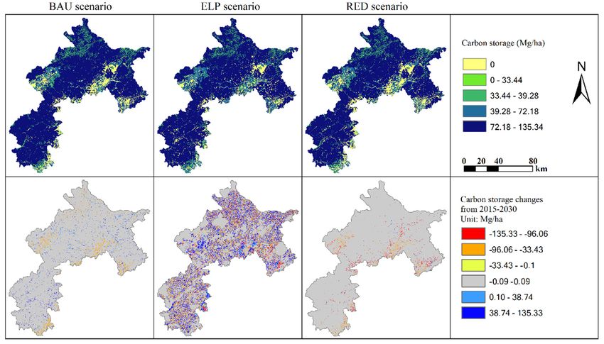
Forests 2020, 11, 584 3 of 20
Beijing”, as well as the “13th Five-Year Plan of Environmental protection and Ecological construction
in Beijing”. Here, we use the ecological conservation area of Beijing, an area with intense human
activities and ecologically vulnerable areas, as the study area. In this area, the complex interaction
between human activities and the natural environment poses a major challenge to the sustainable
provision of ES. Therefore, we first present the future land-use simulation (GeoSOS-FLUS) model and
Markov model to simulate future land use under three alternative scenarios, i.e., Business as Usual
(BAU), Rapid Economic Development (RED), and Ecological Land Protection (ELP) in the ecological
conservation area. Then, we selected the InVEST (Integrated Valuation of Ecosystem Services and
Trade-Offs) model that was developed by the Natural Capital Project team of the United States and
has been widely used in evaluating the quantity of ecosystem services and to support ecosystem
management and decision-making. Specifically, we focus on three main objectives: (1) modeling the
current and future dynamics of the ES—carbon storage (CS), flood regulation (FR), and soil conservation
(SC); (2) quantifying the effects of land-use change on these services and the trade-offs among them;
(3) providing appropriate indicators to support the identification of rational land-use strategies, to
improve ES management for our study area.
2. Materials and Methods
2.1. Study Area
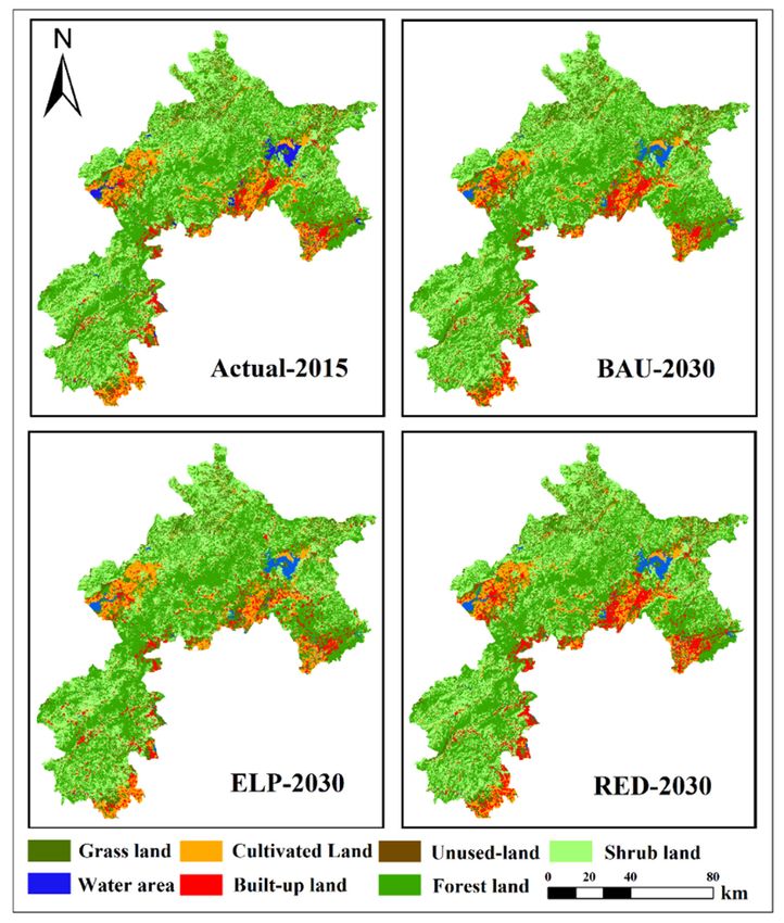
The ecological conservation area (41◦ 040 –39◦ 310 N, 115◦ 240 –117◦ 290 ) is located in Northwestern
Beijing, China (Figure 1). The study area, accounting for approximately 53.3% of the entire area of
the city, covers a total area of 11,140.15 km2 . This region is very mountainous region—with altitudes
varying from 11 to 2304 m—with a typical temperate monsoon climate: average annual precipitation
of 576.71 mm from 2000 to 2015, in which the primary rainfall occurs in the rainy season, from June to
August, and monthly average temperature that ranges from 2.5 to 13.4 ◦ C (Reanalysis of climate data
from the Resources and Environmental Sciences, Chinese Academy of Sciences (http://www.resdc.cn/)).
The ecological conservation area is characterized by rich biodiversity and diverse ecosystems that
include the region’s most important mountain areas, water sources, ecological forests, basic cultivated
land, and other core ecological elements [31]. In recent decades, this region has experienced rapid
urbanization and economic growth, accompanied by increasing environmental concerns [9]. Therefore,
it has been specially protected and identified as a key area in ensuring Beijing’s sustainable development
by the People’s Government of Beijing Municipality.
2.2. Data Requirement and Preparation
Gridded land-use maps of the ecological conservation area in 2000 and 2015 (30 m spatial
resolution) were obtained from the Resources and Environmental Sciences, Chinese Academy of
Sciences (http://www.resdc.cn/). The dataset is based on the supervised classification of Landsat TM
images, using ENVI Imagine software, and uses seven land classes: forest land, cultivated land, water
body, grassland, shrub land, built-up land, and unused land (see descriptions in Supplementary
Table S1). In addition, another five data types were used in the InVEST model: (1) 30 m resolution
SRTM V4.1, Digital Elevation Model (DEM) obtained from National Catalogue Service for Geographic
Information (http://www.webmap.cn/); (2) 1 km resolution meteorological data, including annual
precipitation, monthly precipitation, temperature, and sunshine hours provided by the National Earth
System Science Data Center (http://www.geodata.cn/); (3) 1 km resolution data related to soil attributes,
root restricting layer depth, and plant AWC obtained from the Harmonized World Soil Database
(http://webarchive.iiasa.ac.at/Research/LUC/External-World-soil-database/); (4) evapotranspiration
coefficient (Kc ) values for crops from the Food and Agriculture Organization of the United Nations
(FAO) (http://www.fao.org/3/X0490E/x0490e0b.htm); and (5) carbon stored in the four basic carbon
pools for each land-use type, obtained from previous studies of Beijing City [32]. We used ArcGIS
10.3 for GIS analyses, in which all spatial raster data were converted to the same projection coordinate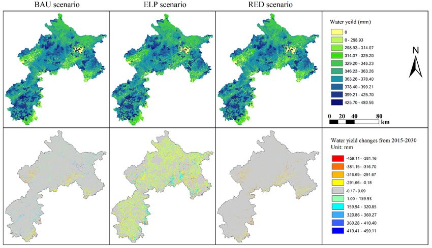
Forests 2020, 11, 584                                                                                        4 of 20

system (Beijing_1954_3_Degree_GK_CM_ 114E) and a spatial resolution of 30 m. The input data are
presented in Table 1.
  Forests 2020, 11, x FOR PEER REVIEW                                                                       4 of 19

                                         Figure1.1.Location
                                        Figure     Location of
                                                            of the
                                                               the study
                                                                   study area.

                          Table1.1.Description
                          Table     Descriptionof of
                                                  thethe
                                                      study datadata
                                                         study   for the
                                                                      forInVEST  model.
                                                                          the InVEST model.
             Data
            Data                       Data Description
                           Data Description                                            Data Sources
                                                                              Data Sources
                        LandLanduse/cover    in in 2000 and 2015 at Resources and Environmental Sciences,
                                     use/cover
 Land                                                 Resources and Environmental        Sciences, Chinese
  Landuse/cover
         use/cover      200030 and   2015  at 30
                                 m spatial resolution
                                                                       Chinese Academy     of Sciences
                                                      Academy of Sciences      (http://www.resdc.cn/)
                                                                       (http://www.resdc.cn/)
                        m spatial resolution
                              Digital Elevation Model with 30 m National Catalogue Service for Geographic
 Digital Elevation ModelDigital Elevation
  Digital Elevation           spatial resolution National Catalogue    Information
                                                                            Service(http://www.webmap.cn/)
                                                                                      for Geographic
                        Model    with precipitation,
                              Annual    30 m            monthly
  Model                                               Information (http://www.webmap.cn/)
                                                                       National Earth System Science Data Center
 Climate data                 precipitation,
                        spatial   resolutiontemperature,               (http://www.geodata.cn/)
                              sunshine   hours
                        Annual precipitation,
                              Soil texture, topsoil sand fraction,
                        monthly                                        Harmonized World Soil Database
                              topsoil silt fraction, topsoil clayEarth System Science Data Center
                                                      National
 Soil  data
  Climate data          precipitation,                                 (http://webarchive.iiasa.ac.at/Research/
                              fraction, root restricting  layer
                                                      (http://www.geodata.cn/)
                                                                       LUC/External-World-soil-database/)
                        temperature,
                              depth, plant AWC
                        sunshine                                       Food and Agriculture Organization of the
                              Plant hours
                                     evapotranspiration for
 Plant evapotranspiration
                        Soil texture,                                  United Nations (FAO) (http:
                              different topsoil
                                        land use/cover types
                                                                       //www.fao.org/3/X0490E/x0490e0b.htm)
                        sand fraction, topsoil
                                                      Harmonized World Soil Database
                        silt fraction, topsoil
  Soil
2.3.    data Scenarios Design
     Future                                           (http://webarchive.iiasa.ac.at/Research/LUC/External-
                        clay fraction, root
                                                      World-soil-database/)
                        restricting
      In this study, land             layerunder three scenarios, was modeled, using the Markov and
                           use in 2030,
                        depth,
future land-use simulation       plant AWC models, which incorporated socioeconomic and ecological
                              (GeoSOS-FLUS)
                        Plant
characteristics in different scenarios [33,34].Food     We used    a 2015 land-use     map asof a the
                                                                                                  baseline  year for
                                                            and Agriculture     Organization          United
  Plant                 evapotranspiration
                                                      Nations (FAO)
  evapotranspiration for different land
                                                      (http://www.fao.org/3/X0490E/x0490e0b.htm)
                        use/cover types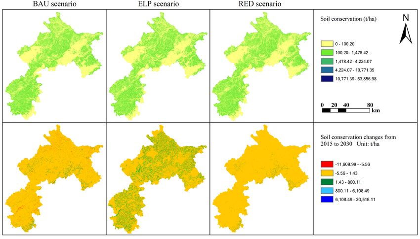
Forests 2020, 11, 584                                                                            5 of 20

comparison under three alternative future scenarios. The climate, including annual temperature and
precipitation, is assumed to maintain the current state.

2.3.1. Business as Usual (BAU)
     We developed the BAU scenario based on the trajectory of land-use transitions over the past 15
years in the ecological conservation area. We assumed that the social, economic, and land-use evolution
trends remain unchanged from 2015 to 2030 under the BAU scenario. Thus, the rate of land-use change
is considered to agree with the annual change from 2000 to 2015 (Supplementary Materials Figure S1
and Table S3). The Markov models were used to simulate the land-use demand.

2.3.2. Ecological Land Protection (ELP)
      The ELP scenario can be viewed as a harmonious development scenario for 2030 that aims to
develop a more human-oriented and sustainable development mode by the local government. This
scenario is characterized by condensed and slower urbanization in which the environment will be
considered. This scenario gives priority to the existing ecological protection measures, including
protecting Miyun reservoir, natural reserves, primary farmlands, and park green spaces, which are
restricted from being converted to other lands. Moreover, under the ELP scenario, the area of built-up
land would show a slight increase and forest land would increase more than other scenarios, up to
2030. The area of cultivated land (paddy fields and dry land) would be held above 7% of the study
area based on the Beijing’s General Urban Planning (2016–2035). This scenario will reduce the speed of
urban growth and the negative effects of urban expansion on ecosystem services.

2.3.3. Rapid Economic Development (RED)
     The RED scenario is based on the BAU scenario but includes rapid urbanization in the study area.
We assumed that rapid increases of population and technologies, as well as economic development,
would occur in the process of urban development from 2015 to 2030, under this scenario. At the same
time, the demands for built-up land, including urban and rural residential land, construction land, and
transport facility areas, would expand rapidly. To be specific, built-up land would be concentrated in
the lower part of the study area and increase more than the other two scenarios. To meet the growing
population’s demand for food, cultivated land will experience less of a decline than the BAU scenario.
In addition, basic farmland protection areas should be added in the restricted area.

2.4. Future Land-Use Modeling
     In this study, we projected different land use for alternative scenarios, using the (1) Markov
model to estimate quantitative demands of different land-uses in 2030 and (2) GeoSOS-FLUS model to
estimate spatial patterns in 2030. The mutual feedback between demand model and GeoSOS-FLUS
model generate the simulated land-use maps at the end of the simulation period [35].

2.4.1. Land-Use Demand Projection
     The Markov model, as a non-spatial demand of future land use, was used to generate the
conversion probability of land-use types over a time series [36,37]. The land-use maps of different
time intervals were exported from simulations and compared with each other, in the form of matrices,
based on maximum values of probability [37,38]. The maximum probability for each grid cell to either
remain unchanged or convert to another class was calculated. Finally, the Markov model was applied
to our study area from 2015–2030, using the probability transition matrix and transition maps of each
class to another class from 2000 to 2015, under the following equation:

                                           Sij (t+1) = Pij Si (t)                                   (1)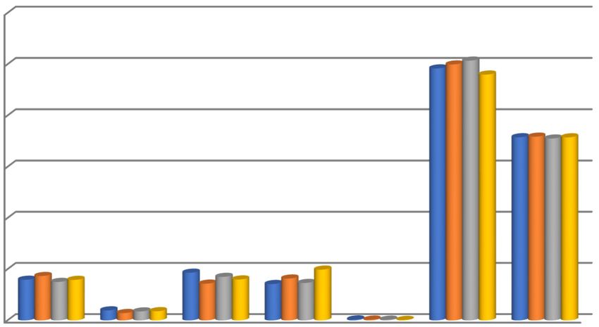
Forests 2020, 11, 584 6 of 20
where Sij(t+1) is the state of land-use type i converting to j at the future time of t+1; Si (t) is the state of
land-use type i at time t; and Pij is the transition probability of land-use type i to j.
2.4.2. Land-Use Spatial Pattern Simulation
The cellular automata (CA) model was designed to project spatial patterns of future land use,
under the given land-use demands determined by the non-spatial module. Within the CA allocation
procedure, the following two steps were implemented: (1) An artificial neural network (ANN) algorithm
was used to train and predict the probability of occurrence of each land-use type on a specific grid [39],
and (2) a self-adaptive inertia and competition mechanism was designed to address the competition
and interactions among different land-use types [34,40]. Driving factors and data of land-use change
were selected from the available literature and tested as predicting variables (Supplementary Table
S2) [34,41].
The ANN was composed of prediction and training stages, whose calculation formula is as
follows: X X 1
sp(p, k, t) = w j,k × sigmoid net j (p, t) = w j,k × (2)
−net j (p,t)
j j 1+e
where sp(p, k, t) is the probability of suitability of land-use type k at time t and grid cell p; w j,k is the
weight between the output layer and the hidden layer; Sigmoid () is the excitation function from the
hidden layer to the output layer; and net j (p, t) is the signal received by the jth hidden grid cell p at
time t. The sum of suitability probabilities of each land-use type output by the ANN is always 1:
X
sq(p, k, t) = 1 (3)
k
In this mechanism, a self-adaptive inertia coefficient for different types of land use is defined to
adjust the difference between current allocated land amount and land demand in the iterative process.
The coefficient of kth land use at time t is Intertiatk , given by:
Intertiat−1
k
Dt−1
k
≤ Dt−2
k
Dt−2
Intertiakt−1 × k
0 > Dt−2 > Dt−1
t
Intertiak
Dt−1
k
k k (4)
Dt−1
Intertiat−1 × k
Dt−1 > Dt−2 >0
Dt−2
k k k
k
where Dt−1
k
and Dt−2
k
are the differences between the demand and allocated amount of land-use type k
at time t-1 and t-2, respectively. By calculating the above two formulas, the probability of land-use
types at each grid cell is estimated, and the dominant land-use type is allocated to this grid cell during
a CA model iteration. The probability TPtp,k of grid p converting to land-use type k at time t is thus
calculated as follows:
TPtp,k = sp(p, k, t) × Ωtp,t × Intertiatk × (1 − scc→k ) (5)
where scc→k is the cost of converting from original land-use type c to the target land-use type k; 1 − scc→k
is the difficulty level of the conversion; and Ωtp,t is the neighborhood effect of land-use type k on grid
cell p at time t.
2.4.3. Model Implementation and Precision Validation
We tested and compared the performance of the FLUS model by simulating land-cover changes
from 2000 to 2015. The land-use spatial distribution in 2000 was regarded as the base map of simulation;
other inputs included the simulation parameters, the restricted areas, and driving data. After running
the GeoSOS-FLUS model for 15 years, a simulated land-use map for 2015 was obtained. We selected
the FoM (Figure of Merit) indicator to measure the performance of the simulation results for land-cover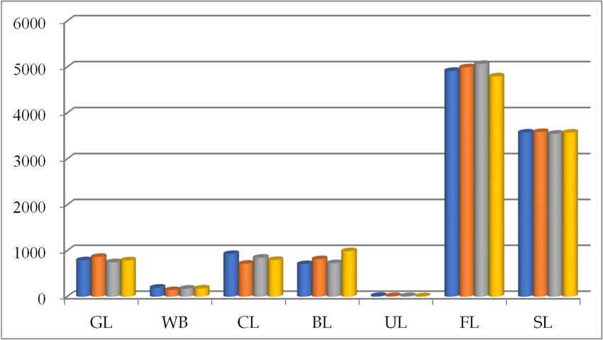
Forests 2020, 11, 584                                                                                 7 of 20

change from 2000 to 2015, as it avoids the disadvantage of overestimating the accuracy in traditional
validation methods (e.g., the overall accuracy and the Cohen’s Kappa coefficient) [42,43]. The FoM can
be mathematically expressed as the ratio of the correct predicted change to the sum of the observed
change and predicted change. The value of FoM, ranging from 0% to 100%, reflects the simulation
accuracy by focusing only on the part of the land that has changed, with 100% representing the perfect
fitting between the observed and simulated changes. The resulting FoM value (0.269) was similar to
or greater than those of other case studies on land-cover-change modeling, as previous comparative
analyses have demonstrated that the common values of FoM ranged from 10% to 30% for existing
land-use-change models [44–46]. This result indicated that the performance of our model was reliable.
Thus, the parameters and driving data within this model are acceptable and can be applied to predict
future land-use patterns (Supplementary Table S2). Hence, we used the abovementioned validated
parameters and the classified land-use map in 2015 to simulate land use in 2030 under three scenarios.

2.5. Quantifying Ecosystem Services
     The current and future ecosystem services (ES) were modeled by using the spatially explicit
InVEST (version 3.8.0.) model, based on land-use maps of current and future scenarios in the ecological
conservation area [47–49]. We focused on the following three ecosystem services: carbon storage (CS),
flood regulation (FR), and soil conservation (SC). These priority ES represent the main and important
categories in relation to climatic, terrain, and soil conditions. The quantification and spatial mapping
of ecosystem services were done within the InVEST model, utilizing a series of parameters and data.

2.5.1. Carbon Storage (CS)
      The amount of carbon stored and sequestered was calculated based on the land-use and climate
information of carbon stocks within each respective time period and simulated scenario, using the tool
“Carbon Storage and Sequestration: Climate Regulation” of the InVEST model. This model aggregates
the amount of carbon stored in four major carbon pools, aboveground biomass, belowground biomass,
soil, and dead organic matter, with land-use maps and particular classification (see Supplementary
Table S4) [49]. We calculated the total carbon stored, CSjxy , for each given grid cell (x,y) with land-use
type, j, as follows:
                                CSjxy = Ax (Cajxy + Cbjxy + Csjxy + Cdjxy )                              (6)

where Cajxy , Cbjxy , Csjxy , and Cdjxy are carbon densities in aboveground biomass (Mg C ha−1 ),
belowground biomass (Mg C ha−1 ), soil (Mg C ha−1 ), and dead matter (Mg C ha−1 ) for the grid
cell (x,y) with land-use type j, respectively.

2.5.2. Flood Regulation (FR)
      Flood regulation service referred to the capacity of a landscape to retain storm-water runoff. The
“Annual Water Yield” module of InVEST model was used to quantify the water yield from each grid
cell, with mean annual precipitation, depth of soil (mm), plant available water content, annual potential
evapotranspiration, and land use (see Supplementary Table S5) [49]. The calculations of annual water
yield, Yx , for each pixel on the landscape x were as follows:

                                           Yx = (1−AETx /Px ) · Px                                       (7)

                              AETx /Px = (1 + PETx /Px ) - [1 + (PETx /Px )ω ]1/ω                        (8)

                                            PETx = Kx · ET0 /Px                                          (9)

                                         ωx = Z · AWCx /Px + 1.25                                      (10)

                        AWCx = Min (Rest. layer. Soil Depth, Root. Depth) · PAWC                       (11)
Forests 2020, 11, 584 8 of 20
where AETxj is the annual actual evapotranspiration for pixel x, and Px is the annual precipitation
on pixel x. AETx /Px is based on an expression of the Budyko curve developed by [50,51]; PETx is
the potential evapotranspiration, and ωx is a an empirical parameter that characterizes the natural
climatic-soil properties; ET0 is the reference evapotranspiration, and Kx is the coefficient of vegetation
evapotranspiration [49]; AWCx is the volumetric plant available water content; and Z is an empirical
constant, sometimes referred to as “seasonality factor”, which ranges from 1 to 30, and needs
to be calibrated with monitoring data from the local precipitation pattern and hydrogeological
characteristics [49]. PAWC is the plant available water capacity (0–1).
2.5.3. Soil Conservation (SC)
The “sediment delivery ratio” module of InVEST model was applied to estimate the annual
processes of catchment soil loss, sediment transport into river channels, and sediment interception
by vegetation and topography, which works on the spatial resolution of the input DEM raster [49].
Following previous studies [52,53], we used the Revised Universal Soil Loss Equation (RUSLE) to
calculate annual soil loss for each pixel, based on the rainfall erosivity and soil erodibility, along with
biophysical attributes related to sediment retention based on land cover. Reductions of soil loss indicate
that there was an improvement in soil conservation. The calculations of SC for pixel i are as follows:
SCi = RKLSi − uslei (12)
uslei = Ri · Ki · Li · LSi · Ci · Pi (13)
RKLSi = Ri · Ki · Li · Si (14)
where SCi is the amount of annual soil conservation (ton·(hm2 ·a)−1 ); RKLSi is the amount of potential
soil loss in pixel i (ton·(hm2 ·a)−1 ); uslei is the amount of actual soil loss in pixel i (ton·(hm2 ·a)−1 ); Ri is
the rainfall erosivity factor (MJ·mm·(ha·hr)−1 ); Ki is the soil erodibility factor (ton·ha·hr·(MJ·ha·mm)−1 );
LSi is the length-gradient factor (unitless); Si is the slope factor (unitless); and Ci and Pi represent
the crop-management and support practice factors (both unitless), respectively (see Supplementary
Table S6).
2.6. Assessment of the Trade-Offs/Synergies among ES
Trade-offs/synergies among ES were expressed with correlation coefficients. First, we applied the
“Create Random Points” tool in ArcGIS 10.3 to create random sample points, and then we extracted the
ecosystem service value of each sample point, using the “Extract Multiple Values to points” method.
The total number of samples selected for this study is 5000. Finally, the correlation coefficients were
calculated by using SPSS 24 statistical software based on the service value of these points (Pearson,
two-tailed).
3. Results
3.1. Changes in Land Use under Different Scenarios
Throughout the duration of the study, most land in the ecological conservation area was predicted
to remain covered by forest and shrub land; however, several transitions were predicted among
land-use types under all three scenarios (Table 2; Figure 2). From 2015 to 2030, land-use-type change is
mainly characterized by built-up land expansion and loss of cultivated, water body, and unused land.
Cultivated and built-up land changes are ranked differently according to the proportion under different
scenarios. As expected, the RED scenario presents the greatest built-up land expansion (+2.52%),
which is much higher than those predicted under the BAU and ELP scenarios (+0.96% and +0.18%,
respectively). The importance of land-use planning and other regulations is clear when comparing
the land-use projections for the ELP and BAU scenarios. For example, under the ELP scenario, theForests 2020, 11, 584 9 of 20
total area of forest land is projected to increase by 152.38 km2 (+1.36%), but the extent of built-up land
and water body remain relatively stable (+20.34 and -20.55 km2 , respectively), and cultivated land
decreases relatively little (-81.39 km2 ).
Table 2. Land-use area (km2 ) and percent area (%) for each land-use type, from baseline year 2015 to
2030, under the BAU, ELP, and RED scenarios in the ecological conservation area.
Types
Forests 2020, 2015 (km2 /%)
11, x FOR PEER REVIEW BAU (km2 /%) ELP (km2 /%) RED (km2 /%)
9 of 19
Grassland 793.74 (7.12) 866.58 (7.78) 751.48 (6.74) 791.36 (7.10)
expansion (+2.52%), which
Water body is much
195.19 (1.75) higher than those
142.92 (1.28)predicted174.64
under(1.57)
the BAU and179.37
ELP (1.61)
scenarios
(+0.96% and +0.18%,
Cultivated land respectively).
931.22 (8.36) The importance
718.01 of land-use planning
(6.44) and other regulations
849.83 (7.63) is clear
799.27 (7.17)
whenBuilt-up land the land-use
comparing 710.49 (6.38) 817.75
projections for the (7.34)
ELP and BAU730.83 (6.56) For example,
scenarios. 991.67 under
(8.90) the
ELPUnused land
scenario, 18.28of(0.16)
the total area forest land is15.24 (0.14) to increase
projected 13.43
by(0.12) 8.83 (0.08)
152.38 km2 (+1.36%), but the
Forest land 4918.48 (44.14) 4995.83 (44.83) 5070.86 (45.50) 4798.94 (43.06)
extent of built-up
Shrub land
land and water body
3576.73 (32.10)
remain relatively
3587.88 (32.20)
stable (+20.34 and -20.55
3552.12 (31.87)
km2, respectively),
3574.94 (32.08)
and cultivated land decreases relatively little (-81.39 km2).
6000 2015 BAU ELP RED
5000
(Area in km2)
4000
3000
2000
1000
0
GL WB CL BL UL FL SL
Figure 2.2.Land-use
Figure Land-usechanges
changes from
from 2015
2015 to 2030,
to 2030, underunder the RED,
the BAU, BAU,andRED,
ELPand ELP scenarios
scenarios in the
in the ecological
ecological conservation area; BL (built-up land), CL (cultivated land), FL (forest land), SL (shrub land),
conservation area; BL (built-up land), CL (cultivated land), FL (forest land), SL (shrub land), UL (unused
UL (unused land), WB (water body), and
land), WB (water body), and GL (grass land). GL (grass land).
Table
The 2. Land-use
increase in built-up 2) and percent area (%) for each land-use type, from baseline year 2015 to
area (kmland occurs at the expense of all other land-use types from 2015 to 2030,
under2030, underscenario,
the RED the BAU,but
ELP, and RED from
especially scenarios in the ecological
the conversion conservation
of cultivated landarea.
and water bodies (Table 3
and Figure 3).Types
Under the BAU and RED scenarios,
2015 (km2/%) BAU (km2/%) the expansion
ELP (km2/%) land
of built-up RED is derived
(km2/%)from the
2
conversion of 134 km of cultivated land alone, which contributes to the decline of cultivated land
Grassland 793.74 (7.12) 866.58 (7.78) 751.48 (6.74) 791.36 (7.10)
from 8.36% to 6.44% and 7.17%, respectively. Under the ELP scenario, forest land expands from 44.14%
Water body 195.19 (1.75) 142.92 (1.28) 174.64 (1.57) 179.37 (1.61)
to 45.50%, largely from conversions from shrub land, grassland, and cultivated land. However, shrub
Cultivated land 931.22 (8.36) 718.01 (6.44) 849.83 (7.63)2 799.27 (7.17)
land declines only slightly under the ELP scenario, as more than 1000 km of forest land and 231.66
Built-up land 710.49 (6.38) 817.75 (7.34) 730.83 (6.56) 991.67 (8.90)
km2 grassland area are converted to shrub land.
Unused land 18.28 (0.16) 15.24 (0.14) 13.43 (0.12) 8.83 (0.08)
Forest land 4918.48 (44.14) 4995.83 (44.83) 5070.86 (45.50) 4798.94 (43.06)
Shrub land 3576.73 (32.10) 3587.88 (32.20) 3552.12 (31.87) 3574.94 (32.08)
The increase in built-up land occurs at the expense of all other land-use types from 2015 to 2030,
under the RED scenario, but especially from the conversion of cultivated land and water bodies
(Table 3 and Figure 3). Under the BAU and RED scenarios, the expansion of built-up land is derived
from the conversion of 134 km2 of cultivated land alone, which contributes to the decline of cultivated
land from 8.36% to 6.44% and 7.17%, respectively. Under the ELP scenario, forest land expands from
44.14% to 45.50%, largely from conversions from shrub land, grassland, and cultivated land.
However, shrub land declines only slightly under the ELP scenario, as more than 1000 km2 of forest
land and 231.66 km2 grassland area are converted to shrub land.Forests 2020, 11, 584 10 of 20
Table 3. Land-use conversion matrix from baseline year 2015 to 2030, under the BAU, RED, and ELP
scenarios in the ecological conservation area (km2 ).
Forests 2020, 11, x FOR PEER REVIEW 10 of 19
Scenarios From 2015 to 2030 GL WB CL BL UL FL SL
GrassWater body (WB) 775.780.05 22.18
land (GL) 141.45 0.85
48.98 0.03
4.36 0.010.28 0.28 6.48 0.25 8.51
Cultivated
Water body (WB) Land (CL)0.05 0.21 141.45
10.32 703.36
0.85 0.86
0.03 0.110.01 1.95 0.28 1.21 0.25
Built-up
Cultivated Landland
(CL)(BL) 0.21 2.19 10.32
10.12 133.99
703.36 660.50
0.86 0.370.11 8.18 1.95 2.41 1.21
BAU Built-up land (BL)
Unused land (UL) 2.19 0.02 10.12 0.01 133.99
0.04 660.50
0.03 0.37 0.09 8.18 0.15 2.41
14.90
Unused land land
Forest (UL) (FL) 0.02 6.09 0.01 10.28 0.04
39.49 0.03
38.05 14.904822.93
1.93 0.09 77.04 0.15
ForestShrub
land (FL)
land (SL) 6.09 9.41 10.28 0.82 39.49
4.52 38.05
6.68 0.681.93 78.564822.933487.2177.04
ShrubGrass
land (SL)
land (GL) 9.41348.83 0.82 2.41 4.52
18.04 6.68
132.36 0.540.68 102.8978.56 3487.21
146.41
GrassWater
land (GL)
body (WB) 348.832.63 2.41 142.76 18.04
3.36 132.36
16.61 0.070.54 6.83102.89 2.38 146.41
Water body (WB) 2.63 142.76 3.36 16.61 0.07 6.83 2.38
Cultivated Land (CL) 19.08 9.25 718.68 16.64 1.92 59.14 25.11
Cultivated Land (CL) 19.08 9.25 718.68 16.64 1.92 59.14 25.11
ELP Built-up land (BL) 11.90 2.60 34.35 420.61 1.13 164.25 95.99
ELP Built-up land (BL) 11.90 2.60 34.35 420.61 1.13 164.25 95.99
UnusedUnused land (UL) 0.04 0.04 0.01
land (UL) 0.01 0.00
0.00 0.01
0.01 13.01
13.01 0.11 0.11 0.24 0.24
Forest land
Forest land (FL) (FL) 179.49
179.49 27.27
27.27 100.19
100.19 82.39
82.39 1.281.283559.24
3559.241121.00
1121.00
ShrubShrub land (SL) 231.66
land (SL) 231.66 10.89
10.89 56.62
56.62 41.85
41.85 0.330.331025.45
1025.452185.33
2185.33
GrassGrass land (GL) 789.46
land (GL) 789.46 0.100.10 0.07
0.07 1.07
1.07 0.030.03 0.57 0.57 0.05 0.05
WaterWater
body body
(WB) (WB) 0.08 0.08 164.27 164.27 0.13
0.13 0.32
0.32 0.200.20 14.2914.29 0.08 0.08
Cultivated Land Land
Cultivated (CL) (CL)0.09 0.09 0.19 0.19 796.15
796.15 1.09
1.09 0.030.03 1.66 1.66 0.06 0.06
RED RED Built-up land (BL)
Built-up land (BL) 3.56 3.56 27.73
27.73 133.95
133.95 689.09
689.09 0.750.75 130.86130.86 5.73 5.73
Unused land (UL)
Unused land (UL) 0.02 0.02 0.01 0.01 0.02
0.02 0.05
0.05 8.508.50 0.16 0.16 0.08 0.08
ForestForest
land (FL)
land (FL) 0.49 0.49 2.80 2.80 0.97
0.97 15.95
15.95 8.048.044767.94
4767.94 2.75 2.75
ShrubShrub
land (SL)
land (SL) 0.05 0.05 0.10 0.10 0.05
0.05 2.95
2.95 0.720.72 2.99 2.99 3568.073568.07
3. Land-use
Figure
Figure maps
3. Land-use of of
maps thethebaseline
baselineyear
year 2015, and2030
2015, and 2030projections
projections under
under the the BAU,
BAU, RED,RED,
and and
ELP scenarios.
ELP scenarios.Forests 2020, 11, 584 11 of 20
Forests 2020,
3.2. Future 11, x FOR
Changes PEER REVIEW
in Ecosystem Services 11 of 19
3.2.1. 3.2. FutureStorage
Carbon Changes in Ecosystem Services
The
3.2.1.total carbon
Carbon storage was 98.92 Tg in 2015, and was predicted to decrease to 96.74 Tg in 2030,
Storage
under theThe RED scenario—primarily caused
total carbon storage was 98.92 by2015,
Tg in rapid urban
and encroachment
was predicted intotocultivated
to decrease 96.74 Tg inand
2030,forest
land (Supplementary
under the RED scenario—primarily caused by rapid urban encroachment into cultivated and forest of
Table S11). The ELP scenario was predicted to result in the highest amount
total carbon storage (100.24
land (Supplementary Tg),
Table due
S11). to ELP
The grassland,
scenarioshrub land, and
was predicted to forest land
result in the expansion
highest amount(+1.27
of Tg).
Foresttotal
land presents
carbon the(100.24
storage highest carbon
Tg), due to storage capacity,
grassland, andand
shrub land, expected 2030expansion
forest land carbon storage values
(+1.27 Tg).
Forest
of 65.42, land and
66.80, presents
63.75theTg
highest
were carbon storage
predicted capacity,
under and expected
the BAU, ELP, and2030
REDcarbon storage values
scenarios, of
respectively
65.42, 66.80, and 63.75 Tg were predicted under the BAU, ELP, and RED scenarios,
(Supplementary Table S7). The transition from forest to built-up land leads to the greater loss of carbonrespectively
(Supplementary
storage under the ELP Table
andS7).
REDThescenarios,
transition from forest to (Supplementary
respectively built-up land leadsTable
to theS11).
greater loss of
Furthermore,
carbon storage under the ELP and RED scenarios, respectively (Supplementary Table S11).
carbon storage growth was distributed predominantly on the periphery of grassland, cultivated land,
Furthermore, carbon storage growth was distributed predominantly on the periphery of grassland,
and shrub land due to the expansion of forest land and shrub land (Figure 4).
cultivated land, and shrub land due to the expansion of forest land and shrub land (Figure 4).
FigureFigure 4. Top,
4. Top, spatial
spatial distributions
distributions ofofcarbon
carbonstorage
storage (CS),
(CS), and
andbottom,
bottom,spatial distributions
spatial of changes
distributions of changes
in CS in CS from
from baseline,
baseline, in 2030,
in 2030, under
under thethe BAU,RED,
BAU, RED,and
and ELP
ELP scenarios.
scenarios.
3.2.2. 3.2.2.
Flood Flood Regulation
Regulation
The total
The total flood flood regulation
regulation capacitywas
capacity waspredicted
predicted to
to decrease
decreasefrom fromthe 2015
the 2015baseline (350.37
baseline ten ten
(350.37
million
3 m3) to 2030, under the BAU, ELP, and RED scenarios (Supplementary Table S8). In 2030, the
million m ) to 2030, under the BAU, ELP, and RED scenarios (Supplementary Table S8). In 2030, the
total predicted amount of water yield under RED scenario will have the highest totaling water yield
total predicted amount of water3 yield under RED scenario 3will have the highest totaling water yield
(totaling 352.26 ten million3 m ), which is +1.89 ten million m 3more than 2015 and has the lowest flood
(totaling 352.26 ten million m ), which is +1.89 ten million m more than 2015 and has the lowest flood
regulation ability (Supplementary Table S8). The transition from cultivated land and forest land to
regulation
built-upability (Supplementary
land triggered increased Table S8). The
water yield transition
under from cultivated
the RED scenario. land and
The ELP scenario willforest land to
be + 0.12
built-up land triggered increased water yield under the RED scenario. The ELP scenario
ten million m compared to 2015 (totaling 350.49 ten million m ), due to the transition from grassland,
3 3 will be + 0.12
ten million 3
m compared to 2015 (totaling 3
cultivated land, and shrub land to forest350.49 ten million
land. Among all of m
the),land-use
due to the transition
types, the floodfrom grassland,
regulation
of built-up
cultivated land,land
and isshrub
projected
landtotohave theland.
forest highest increase,
Among allfrom 26.83
of the ten million
land-use m3the
types, to 36.81
floodten million of
regulation
m3 (9.98
built-up landten million m3to
is projected ) by 2030,
have theunder the RED
highest scenario,
increase, fromdue to the
26.83 tenincrease 3 to 36.81
millioninmbuilt-up land
tenarea
million
m (9.98 ten million m ) by 2030, under the RED scenario, due to the increase in built-up landflood
3 and low flood regulation
3 capacity (Supplementary Tables S8 and S11). The changes of area and
regulation are mainly distributed in the transition zones between forest and shrub land, under the
low flood regulation capacity (Supplementary Tables S8 and S11). The changes of flood regulation
ELP scenario, because of the high runoff coefficient of built-up land and cultivated land (Figure 5).
are mainly distributed in the transition zones between forest and shrub land, under the ELP scenario,
Under the other two scenarios, flood-regulation changes are mainly distributed around cities,
because of the high runoff coefficient of built-up land and cultivated land (Figure 5). Under the other
cultivated land, and water bodies.
two scenarios, flood-regulation changes are mainly distributed around cities, cultivated land, and
water bodies.Forests 2020, 11, 584 12 of 20
Forests 2020, 11, x FOR PEER REVIEW 12 of 19
Forests 2020, 11, x FOR PEER REVIEW 12 of 19
Figure
Figure 5. Top,
5. Top, spatial
spatial distributions
distributions of flood
of flood regulation
regulation (FR),(FR), and bottom,
and bottom, spatial
spatial distributions
distributions of
of changes
changes in WY from baseline, in 2030 under the BAU, RED, and
in WY from baseline, in 2030 under the BAU, RED, and ELP scenarios. ELP scenarios.
Figure 5. Top, spatial distributions of flood regulation (FR), and bottom, spatial distributions of
3.2.3. Soilchanges
3.2.3. in WY from baseline, in 2030 under the BAU, RED, and ELP scenarios.
Conservation
Soil Conservation
TheThe
3.2.3. Soilpredicted
predicted soil
Conservation soil conservationexhibited
conservation exhibited disparate
disparate patterns
patternsunder under thethe
BAU BAU compared
compared to ELP
to ELP
and and
REDRED scenarios
scenarios (Supplementary
(Supplementary Table
Table S9).Under
S9). Underthe theBAUBAU scenario,
scenario, soilsoil conversion
conversionisispredicted
predicted to
The predicted
to decrease soil ten
conservation exhibited disparate patterns
millionunder the BAU compared to ELP
decrease from from
246.86 246.86
ten million milliontons tonsin in 2015
2015 toto246.74
246.74tenten million tons
tonsinin2030,
2030, a decline
a decline of 0.12 ten ten
of 0.12
and RED scenarios (Supplementary Table S9). Under the BAU scenario,
million tons, due to the conversion from cultivated land to grass land and forest land to shrub land soil conversion is predicted
million tons, due
to decrease fromto246.86
the conversion
ten million from
tons cultivated
in 2015 landten to million
grass land and forest land to of shrub tenland
(Supplementary Table S11). The ELP and RED to 246.74
scenarios predict antons in 2030,
increase of 3.4a decline
ten million 0.12tons
(Supplementary
million Table S11). The ELP and RED scenarios predict an increase of 3.4 ten million tons
land and
and 1.88tons, due to the
ten million tons,conversion
respectively, fromwhich
cultivated
couldland to grass land
be attributed to the andtransition
forest land fromto shrub
cultivated
1.88 (Supplementary
ten million tons, respectively, whichand could bescenarios
attributed to thean transition from cultivated land and
land and forest Table S11). The
to built-up landELP RED
(Supplementary Tablepredict
S11). Under increase
the ELPof 3.4 ten million
scenario, the tons
soil
forest
conservation of shrub land showed the greatest decline—from 97.12 ten million tons to 87.94 ten of
andto built-up
1.88 ten land
million (Supplementary
tons, respectively, Table
which S11).
could Under
be the
attributedELP toscenario,
the the
transition soil
from conservation
cultivated
shrub land
land
million showed
and forest
tons; the
however, greatest
to built-up
the largedecline—from
landconversion
(Supplementary97.12 ten million
Table
from shrub S11).
land tons
to Underto 87.94
forest the ten
land ELP million
offsets scenario, tons;thehowever,
this deficiency.soil
conservation
the large
Despite of shrub
conversion
the overall from land
shrub
increase inshowed
land
soil tothe greatest
forest
conservation land decline—from
offsets
in 2030, thisthe
under 97.12
deficiency. ten Despite
RED scenario, million tons to 87.94
the spatial
several overall ten
increase
areas
million
in soil
experience tons;
conservationhowever,
a decline in the
in 2030, soil large
under conversion
the
conservation REDdue from
scenario,
mainlyshrubto aland
several to forest
spatial
reduction land
areas
of forest offsets
experience thisa deficiency.
land, cultivateddecline in soil
land,
Despite
conservation the
and water due overall
bodies increase
mainly
(Figure to 6).in soil
a reduction conservation
Among allofofforest in 2030, under
land, cultivated
the land-use the
types, shrub RED
land, scenario,
landand several
waterthe
presents spatial
bodies
highest areas
(Figure
soil 6).
experience
conservation
Among a capacity,
all of the decline
land-use inwith
soil conservation
an
types, average
shrub land due
quantity mainly tot/km
of 4.80the
presents ahighest
reduction
2 in 2015 and
soil ofconservation
forest land,2 in
5.54 t/km cultivated
2030.
capacity, land,
with an
and water bodies (Figure 6). Among all of the land-use types, shrub land presents the highest soil
average quantity of 4.80 t/km2 in 2015 and 5.54 t/km2 in 2030.
conservation capacity, with an average quantity of 4.80 t/km2 in 2015 and 5.54 t/km2 in 2030.
Figure 6. Top, spatial distributions of soil conservation (SC), and bottom, spatial distributions of
changes in SC from baseline, in 2030, under the BAU, RED, and ELP scenarios.
Figure
Figure 6. Top,
6. Top, spatial
spatial distributionsofofsoil
distributions soil conservation
conservation (SC),
(SC),and
andbottom,
bottom,spatial distributions
spatial of of
distributions
changes in SC from baseline, in 2030, under the BAU, RED, and ELP scenarios.
changes in SC from baseline, in 2030, under the BAU, RED, and ELP scenarios.Forests 2020, 11, 584 13 of 20
3.3. Trade-Offs and Synergies among Ecosystem Services
We performed correlation analyses between pairs of ES, to explore the trade-offs and synergies in
the ecological conservation area during the period from 2015 to 2030 (Table 4 and Supplementary Table
S10). The trade-offs and synergies were identified by the correlation coefficient. Carbon storage (CS)
and soil conservation (SC) would be positively correlated with each other throughout the period from
2015 to 2030, indicating the existence of synergistic effect between these two ecosystem services. At
the same time, it also suggests the high capacity of forest and shrub land in sequestering carbon and
regulating water runoff in the ecological conservation area. The correlation between carbon storage
and soil conservation presented the strongest under the ELP scenario, and the correlation coefficient
was 0.642. The positive relationship between soil conservation (SC) and flood regulation (FR) from
2015 to 2030, under the ELP scenario, respectively, proved the existence of synergies. In addition,
carbon storage was not correlated with flood regulation in 2015, but these two ecosystem services
would be positively correlated under the BAU, ELP, and RED scenarios. This implies that ecological
land, including forest land and shrub land, will become increasingly important in regulating water
balance in the future.
Table 4. Correlation analysis between pairs of ecosystem services in ecological conservation area in the
year 2015. Supplementary data for the correlation analysis in the year 2030 under different scenarios
are in Supplementary Table S10.
Carbon Storage Flood Regulation Soil Conservation
Carbon storage 1 0.003 0.528 **
Flood regulation 1 0.029 **
Soil conservation 1
** p < 0.01.
4. Discussion
4.1. Response of Ecosystem Services to Land-Use Changes
In this study, we found major changes in land-use analysis over the period from 2015 to 2030,
under three alternative scenarios, including rapid expansion of built-up land, increase of forest and
grassland, and sharp declines in cultivated land, water bodies, and unused land. The impacts of these
changes on ecosystem services vary in direction and magnitude under different development scenarios.
For instance, the expansion of built-up land can result in decreased supply to multiple ecosystem
services—carbon storage and flood regulation [54,55], as our results show during the conversion from
forest and cultivated land to built-up land under the BAU and RED scenario. Generally, ecosystems
changing from high vegetation cover to low vegetation cover will exhibit decreased carbon storage
and water conservation [14,56,57]. When compared with other land-use types, forest land was the
major carbon sink. It also suggests that the necessity of ecological protection projects in our study area.
However, we also find that the conversion of shrub land and unused land to built-up land can lead to
beneficial effects, such as stabilization of sand and reduction of soil erosion, as has been previously
reported [32,58].
The flood regulation and soil conservation provided by different land-use classes are associated
with natural and physical conditions, such as climate, soil, and geology. For instance, our result shows
that the conversion from forest land to grassland or shrub land generally resulted in a decrease in
carbon storage, soil conservation, and flood regulation. On the one hand, due to the lower plant
density and root depth, grassland and shrub ecosystems have less regulating capacity on rainfall
than forest ecosystems, so the lower water percolating capacity of grassland and shrub land results
in a relatively low flood regulation. In addition, previous researches have shown that vegetation
plays an important role in controlling soil erosion by intercepting rainfall, increasing infiltration, and
stabilizing the soil [32]. On the other hand, forest land going to grassland will lead to increased soilForests 2020, 11, 584 14 of 20
erosion because of the steep terrain and heavy rainfall, which are prone to landslides, mudslides, and
other geological hazards in the mountain zone, and therefore threaten grazing, tourism, etc. [59,60].
Therefore, soil erosion is more likely to occur under the BAU and RED scenarios. On the contrary,
the conversion of grassland and cultivated land to forest land resulted in a greater increase in carbon
storage and soil conservation, especially under the ELP scenario. This can be explained that the strict
spatial regulations of the ELP scenario that forbid the conversion of the Miyun reservoir and 21 nature
reserves, according to the “Beijing’s General Urban Planning (2016–2035)”.
Our study also shows that, in addition to the differential ES provision, land-use changes will affect
trade-offs and synergies among ES. For example, gains in soil conservation typically result in increased
flood regulation in 2015 and 2030 under the ELP scenario. It could be explained that forest cover
accounting for the largest proportion under the ELP scenario will protect soil surfaces from rainfall and
promote flood regulation increase, but possibly lead to water scarcity. In addition, when shrub land
is converted to grassland, flood regulation shows a decrease trend, in contrast with carbon storage
and soil conservation, consistent with [61]. Therefore, the conversion between land-use types in the
ecological conservation area must be managed carefully. Forest has played an important role in local
and regional climate regulation and water conservation [62]. Thus, although urban expansion may
boost the regional economy, the conversion of forest land to built-up land will likely lead to great losses
of climate and flood regulation services. Therefore, the study of the correlations between land-use
changes and ES trade-offs warrant further investigation [63,64].
4.2. Strategies and Implications
We propose the maximizing ecological benefits (ELP) scenario for the ecological conservation
area. In comparison to the other two scenarios, we predict that the BAU scenario presents a number of
undesirable environmental outcomes. Water reserves, natural reserves, and several national forest
parks are forbidden to convert to other land uses under the ELP and RED scenarios in compliance
with ecological protection plants. Our results indicate that the expansion of built-up land will be
effectively controlled, with less natural or semi-natural ecosystems being converted to built-up land
under the ELP scenario. The RED scenario showed an increase in soil conservation, but decreases in
carbon storage and flood regulation compared to the BAU scenario. These trade-offs are the issues
that urban planners face as they chart out a future for growing cities. The ELP scenario should be a
future priority because it takes into account the land needed to meet the multitude of resources and
growing population demands, as proposed in the “Beijing’s General Urban Planning (2016–2035)”.
Therefore, we suggest that the People’s Government of Beijing Municipality should strengthen the
implementation of natural resources protection planning and spatial control, to effectively alleviate
ecosystem degradation.
Our study has identified hotspots of ecosystem-service gains and losses that respond to land-use
changes, allowing us to proscribe cost-effective land-use spatial regulations for maintaining and
enhancing ecosystem services. We further propose four major strategies that may be used as guidelines
for improving ecosystem services in the ecological conservation area. First, and most importantly,
more efficient use of current urban land resources should be adopted, such as more compact buildings
and redevelopment of discarded factories, as suggested by [9,16]. Second, high-quality cultivated land,
especially basic farmland, should be strictly protected from urban expansion, to ensure adequate food
supply. Third, trees, especially along primary roads, should be enhanced, as the increase in forest cover
will promote the regional spatial balance of carbon storage in these areas in the future [65]. Finally, we
must improve the utilization of water resources; most precipitation is transported into urban sewers
and cannot be easily used by human beings [66,67]. In conclusion, through wise land-use management,
the win-win development patterns of natural ecosystems and socioeconomic systems can be realized
in the future.Forests 2020, 11, 584 15 of 20
4.3. Strengths and Limitations
As mentioned above, the main components of our study were land-use simulation and ecosystem
services evaluation. Our methodology provides a straightforward and flexible way to explore possible
implications of land-use change for ecosystem services under future land-use conditions. Another
strength is that these results will inform researchers and policymakers as they draft appropriate
measures to better adapt to different future scenarios [68]. However, some limitations always exist in
future land-use simulation, and this is true for our analysis of the ecological conservation area. For
instance, the GeoSOS-FLUS model transition rules (referring primarily to the conversion cost and the
well-trained ANN model) are assumed to be unchanged during the simulation process, while these
rules may change at a certain time in the future (e.g., 30 or 50 years), in the real world [69].
The InVEST model applied here has been widely used for assessing ecosystem services across
multiple time scales [56,70,71]; however, we also recognize its modeling and data limitations. Firstly,
the results for evaluating ES are dependent on the land-use classifications used. Here we classify land
use into seven broad classes, in which all types of minor lands are assumed homogeneous. For example,
carbon storage capacity within a forest landscape is affected by temperature, elevation, rainfall, and
forest age, which were not captured by our classification scheme. Secondly, although we used land-use
maps derived from 30 m resolution remote-sensing images, other data, including soil, precipitation,
and temperature were available only at 1000 m resolution, which increases the uncertainty of ecosystem
service evaluation. Thirdly, the “Annual Water Yield” module is based on annual averages, which
neglect extrema and does not consider sub-annual patterns of water delivery timing [72]. Finally,
given the simplicity of the InVEST model and small number of parameters, the output results of the
“sediment delivery ratio” module are very sensitive to most input parameters [73]. Therefore, the
errors of the empirical parameters of the USLE equation will have a great effect on our predictions.
The purpose of this study was to explore the impacts of land-use change on ecosystem services
under different scenarios, which can provide information for the formulation of land-use policy. Given
this objective, climate remains constant from 2015 to 2030, leaving land-use change as the sole driver
affecting changes in ecosystem services. Assessing the impact of climate and land-use changes on
ecosystem services is valuable, as they have been identified as the two main factors driving the
provision of ES and trade-offs [74]. Among them, climate change impacts on ES by modifying the
biophysical processes of ecosystems. Although there have been some studies exploring the relative
importance of land use and climate on ES [70,75,76], how the different climate models incorporate
land-use policies is still a challenge in the future. Therefore, our next work will focus on the relative
and combined effects of climate and land-use changes on ES and trade-offs among multiple ES under
different scenarios in the future.
5. Conclusions
In this study, we explored how land-use changes would affect ecosystem services, including carbon
storage, flood regulation, and soil conservation, from 2015 to 2030, under three different scenarios.
According to our results, the significant increase of built-up land is mainly at the expense of the water
bodies and cultivated land in 2030, under the BAU and RED scenarios. The ELP scenario would show
the largest increase in forest land, and the change of cultivated land and built-up land is relatively
stable compared with the other two scenarios, due to the strict protection policy on ecological land. As
a result, the ELP scenario would show the highest amount of carbon storage, flood regulation, and
soil conservation. The cultivated land and forest land converted to built-up land would promote soil
conservation, but trigger greater loss of carbon storage and flood regulation capacity. We also found
trade-offs or synergies among ecosystem services in which carbon storage would show significant
positive correlation with soil conservation from 2015 to 2030. Based on these findings, we propose
four major land-use strategies, including fully utilizing urban land, farmland protection, tree planting,
and utilization of water resources to achieve sustainable use of ecosystem services in the ecological
conservation area.You can also read