Eco environmental assessment model of the mining area in Gongyi, China
←
→
Page content transcription
If your browser does not render page correctly, please read the page content below
www.nature.com/scientificreports
OPEN Eco‑environmental assessment
model of the mining area
in Gongyi, China
Ying Wang1,2, Xueling Wu1*, Siyuan He1 & Ruiqing Niu1
The ecological environment directly affects human life. One of the ecological environmental issues
that China is presently facing is deterioration of the ecological environment due to mining. The
pollution produced by mining causes the destruction of land, water bodies, the atmosphere, and
vegetation resources and new geological problems that seriously impact human civilization and life.
The main purpose of this study is to present an environmental assessment model of mine pollution
to evaluate the eco-environment of mining. This study added mineral species and mining types into
the factor layers and built an improved evaluation system to accurately evaluate the impact of mines
on the eco-environment. In the non-mining area, the grades of the eco-environment were divided
according to the Technical Criterion for Ecosystem Status Evaluation standard document. In the
mining area, the grades of the assessment for the eco-environment were classified by a field survey.
After comparing the accuracy of various methods, the support vector machine (SVM) model, with an
accuracy of 94.8%, was chosen for the mining area, and the classification and regression tree (CART)
model, with an accuracy of 89.36%, was chosen for the non-mining area. Finally, environmental
assessment maps for the entire study area were generated. The results indicate that the mine
environmental assessment system established by this study avoids the subjective limitations of
traditional assessment methods, provides an effective method for assessing ecological quality, and
will help relevant departments to plan for mine resources.
The ecological environment refers to the sum of various natural forces (materials and energy) or actions that
are closely related to human life and production activities. Mining is considered an important driving force
for geological environmental problems, including geological disasters, environmental pollution, and resource
destruction1,2. Thus, the ecological security of mining areas has become an important research topic. Mine
development areas generally have complex terrains and diverse features, and obtaining information on the
land features can be difficult. In recent years, researchers have used the multi-sensor, multi-spectral, and multi-
temporal advantages of remote sensing (RS) technology, combined with other relevant data, to conduct dynamic
surveys of the development status of mineral resources and the mining eco-environment3. RS technology has the
characteristics of fast information acquisition, short period and large coverage, and the acquisition of information
is less restricted by conditions. Therefore, it can quickly and extensively monitor the ecological environment of
a mining area, which has advantages over traditional methods.
During the long-term development of mineral resources, the negative impacts of various geological environ-
mental problems induced by mining activities on the regional eco-environment have been neglected. Thus, seri-
ous geological environmental problems have accumulated, such as landscape destruction, vegetation destruction,
and water and soil loss; excessive groundwater drainage, resulting in a decline in the regional groundwater level
and destruction of the water resource balance; excessive land use for waste soil, waste rock, and waste slag; and
ground subsidence, ground fissures, mountain collapse, landslides, and other secondary geological disasters4.
The more serious geological environmental problems that have occurred in mines are mainly distributed in
Gongyi city, Henan Province, China, as follows: (1) open-pit mines, which have a large number of extraction
wells, cause extremely serious land destruction; (2) large amounts of stripped waste are randomly discharged,
and mudslides are easily triggered in the rainy season; and (3) cracks in the mountains are liable to induce
collapses and landslides, in addition to other serious geo-environmental problems and hidden h azards5. Large
amounts of tailings are used for stripping and processing gravel, and along the slope, landslides, and debris flow
1
Institute of Geophysics and Geomatics, China University of Geosciences, Wuhan 430074,
China. 2School of Environmental Science and Engineering, Southern University of Science and Technology of
China, Shenzhen 518055, China. *email: snowforesting@163.com
Scientific Reports | (2021) 11:17549 | https://doi.org/10.1038/s41598-021-96625-9 1
Vol.:(0123456789)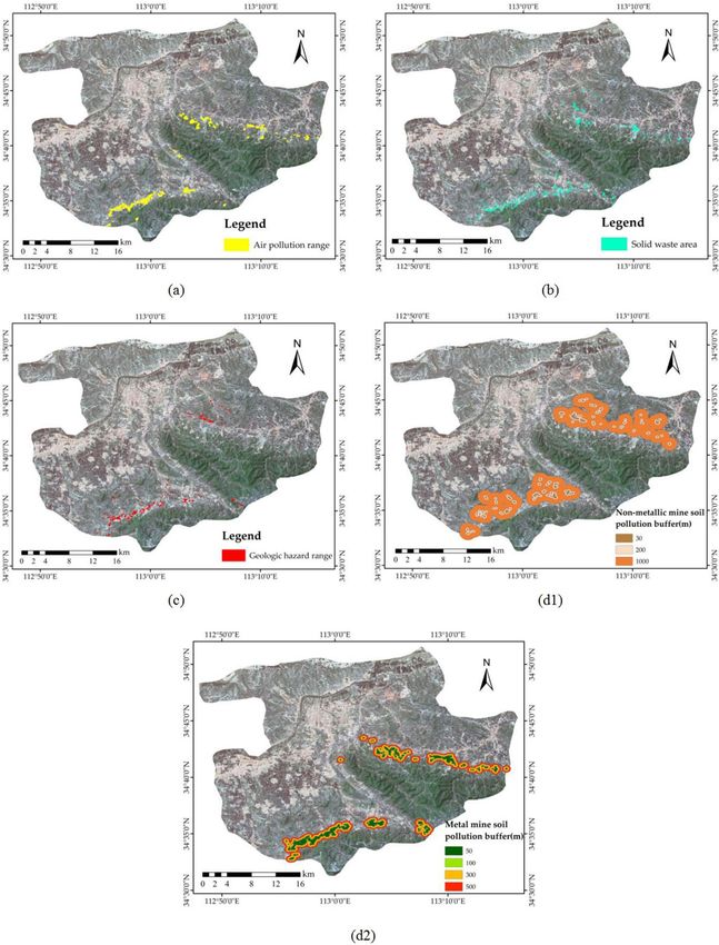
www.nature.com/scientificreports/
disasters are easily triggered; in the mining and processing areas, the environment is seriously damaged, and
dust pollution is prominent.
Relying on conventional methods, such as ground surveys, is very expensive and time consuming for deter-
mining the source and extent of environmental pollution6. Zhao et al. studied the level of heavy metal pollution by
measuring the chemical composition of soil in coal mining areas7. However, the chemical measurement method
is not practical for large-scale detection. The continuous improvement of geographic information system (GIS)
applications and RS has increased opportunities for environmental data a nalysis8. Many studies have used GIS
and RS for environmental assessment, and many methods can be combined with GIS and RS for environmental
evaluation9. Xu et al. took the coal mining area as a case area and presented a method of monitoring and assess-
ing landscape ecological quality using a landscape ecological assessment model based on landscape ecological
theories, remote sensing and geographic information systems t echnology10. Studies in Morocco by Khalil et al.11
have shown that integrating multi-disciplinary data and using GIS techniques is more efficient than traditional
methods in assessing the impact of abandoned mines on the environment and predicting the process of pollution.
For the research conducted at the Dexing mine, Jiangxi P rovince12, the water colour, mine acreage and mineral
residue locations and the variation in the plant coverage within 1 km around the water system were defined as
the index indicators. The methods used to calculate these index indicators are also illustrated and are based
on primary geographical information and RS data. For example, digital elevation model (DEM) data are often
included in the ASTER GDEM V2 dataset, and land type information can be obtained from most RS images.
The quality of the environment can be evaluated in many ways. Traditional methods, such as fuzzy compre-
hensive evaluation (FCE), the comprehensive index method (CIM), and the analytic hierarchy process (AHP),
are widely used in multi-factor comprehensive evaluation methods because of their ease of handling13–15. For
example, the AHP model was combined with GIS, and the coastal mining city Longkou was used as a research
area to evaluate the geological and eco-environmental quality based on spatiotemporal big data16. However, these
evaluation results are subjective in determining the evaluation weights17. Wang and Li used the influence of the
mining construction process, natural eco-environment, and social economic environment as the indicators in
the mining environment assessment, using rank correlation analysis (G1 method) to obtain the assignment for
weight and build a single-mine environmental quality evaluation s ystem18. The support vector machine (SVM)
model and the classification and regression tree (CART) model are also often used to generate predictions based
on large amounts of data. For instance, the SVM algorithm was designed to classify land use types in mining areas
and provides good classification a ccuracy19. This reflects the advantages of the SVM in classification problems.
In terms of environmental assessment, a study on soil environmental assessment in Guizhou, China, found that
the SVM model was superior to the FCE and Nemerow comprehensive pollution index methods because it is
more in line with the actual situation20. Li Dong et al. concluded that the SVM model was less prone to errors and
faster than the back propagation (BP) neural network model when simulating the nonlinear relationship between
various factors in the mine and conducting environmental evaluation21. The CART model can help improve the
accuracy of metal contamination assessments to nearly 90% and can be used to study the relationship between
metal pollution and human variables22. Since these machine learning methods have shown their advantages of
low manual intervention and high efficiency, they have been increasingly used in environmental assessment.
In this study, the main purpose was to propose a mine pollution environment assessment model. Taking the
Gongyi city mining area as an example, a widely used intelligent algorithm evaluation model was obtained. After
using remote sensing images to interpret the mine information, DEM, soil type, land use type and meteorological
data were used to generate the factor layer after preprocessing. Mineral types and mining types were added to
the factor layer, and an improved evaluation system was established. The entire study area was divided into two
parts, the mining area and the non-mine area, according to the mining area and government planning. Different
intelligent models were used to predict environmental assessments across the whole study area. This method
avoids the limitations of traditional sampling methods and reduces the subjectivity of empirical models. This
work provides an efficient method for evaluating ecological quality and will help future resource development
and mining planning.
Study area
Zhengzhou city is the capital of Henan Province, located in the hinterland of the Central Plains and among the
nine states of China (Fig. 1b), and it is a political, economic, and cultural centre in Henan Province. Zhengzhou
is known as the “heart” of the railways of China, and its road traffic extends in all directions. Additionally,
Zhengzhou city is rich in mineral resources23; mining accounts for an important proportion of the total indus-
trial output from the city and has become the main industrial economic pillar of Zhengzhou city. Gongyi city is
part of Zhengzhou city and is located in the northern foothills of Mount Songshan, 82 kms east of Zhengzhou
(Fig. 1c). Gongyi is situated between latitudes 34°31′–34°52′N and longitudes 112°49′–113°17′E and is 43 kms
long from east to the west and 39.5 kms wide from north to south, with a total area of 1052 km224. Gongyi city is
located in a warm temperate continental monsoon climate. The annual sunshine time is approximately 2400 h,
and the average temperature is between 14.3 and 14.8 °C, which can meet the industrial production d emand25.
The average annual precipitation is 583 mm, and the precipitation is mostly concentrated in July, August and
September (accounting for 70% of the whole year). In terms of landform types, Gongyi is low in the north and
high in the south, with mountains, hills, and plains. Gongyi city is rich in mineral resources. At the end of 2017,
21 types of minerals were discovered in the city, including coal, iron ore, bauxite, gallium ore, limestone, refrac-
tory clay, ceramic clay, pyrite, bauxite, etc. The main problems of the mine geological environment in Gongyi
are the destruction of the topography and landscape caused by open and underground mining, the occupation
and destruction of land resources, the geological disasters induced by mining activities, and the destruction of
Scientific Reports | (2021) 11:17549 | https://doi.org/10.1038/s41598-021-96625-9 2
Vol:.(1234567890)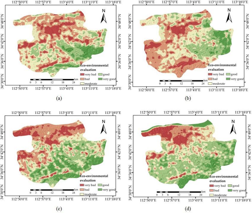
www.nature.com/scientificreports/
Figure 1. Location of the study area in China. (a) Map of China; (b) map of Henan Province; and
(c) Gaofen-2 (GF-2) satellite image (http://www.hbeos.org.cn/) showing the location of Gongyi.
The Figure is created using ArcGIS ver.10.3 (https://www.esri.com/).
aquifers by underground mining activities. The four maps in Fig. 1 show the geographical locations of China,
Henan Province, Zhengzhou and Gongyi (Fig. 1).
Data
Mine data. Mine data, such as mine distribution data, mine type data, and mining method data, were
obtained by visual interpretation from Gongyi’s high spatial resolution RS image data. High-resolution remote
sensing data show the true shape, size, colour and other information of objects on the surface of the earth. The
texture information of ground objects is abundant and can be used to better analyse dynamic changes and moni-
tor the environment. These RS image data were collected from the GF-2 satellite, which is the first civil optical
RS satellite in China, with a spatial resolution up to 0.8 m, independently developed by China. The resolution of
GF-2 data is 0.81 m for panchromatic data and 3.24 m for multi-spectral d ata26. This study used a high-quality
GF-2 RS image on May 21, 2016, because the image of this day has no cloud coverage and high image quality
in this area. The impact of mining on surface changes is not obvious on satellite images. The information on the
scale and type of mining reflected by a high-quality remote sensing image is representative for a long period of
time, so we only used a clear image to acquire the mining information. This RS image was then preprocessed
using atmospheric correction, orthorectification, and geometric correction. After the fusion process, the final
image spatial resolution is 1 m. The government provided the mining scope, minerals (metallic minerals or non-
metallic minerals) and mining methods (open-pit mining or underground mining) reported by mine owners.
The metal mines in Gongyi city are mainly bauxite and iron ore, and the non-metallic mines are mainly coal
mines, with a few limestone mines. We conducted the visual interpretation of the mine on the GF-2 RS images
according to the minerals and mining methods within the specified mining scope. Visual interpretation relies
on the knowledge and experience of the interpreter to identify the mine type and range information from the
remote sensing images, establish the interpretation marks, use ArcGIS software to draw out the mining area
vector and set the attribute table. In the GF-2 RS image, the spots of different mine types differ in colour, size,
and texture, and some have obvious mining equipment and houses. Then, 100 training sampling points were
randomly selected. To ensure that each mine type was included, we randomly sampled each type proportionally.
After the field investigation at the sampling points, the interpretation marks of each type of mine were sum-
marized, and all original interpretation results were modified. In the modified interpretation map, we obtained
the following results: the mine types in the metal mine mainly include stopes, concentrator plants, ore piles, and
tailings ponds, and the mine types in the non-metallic mine mainly include stopes (open pits), concentrator
plants, dumping sites, coal piles, and ore piles (Fig. 2).
Socio‑natural factors. Social and natural factors were gathered according to the official government docu-
ment HJ 192–2015 on the eco-environment assessment. These factors included DEM-derived factors, meteor-
ological-derived factors, and land type factors (Fig. 3). The DEM data were obtained by processing the ASTER
GDEM V2 dataset and have a resolution of 30 m. Elevation and slope data were extracted from the DEM data by
Scientific Reports | (2021) 11:17549 | https://doi.org/10.1038/s41598-021-96625-9 3
Vol.:(0123456789)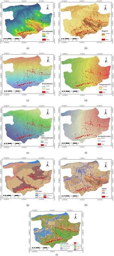
www.nature.com/scientificreports/
Figure 2. Mine interpretation and field investigation. (a) Map of Gongyi; (b) maps of the mine interpretation
on Xiaoheimeigou Mountain. The Figure is created using ArcGIS ver.10.3 (https://www.esri.com/).
using the ENVI and ArcGIS software packages. Meteorological-derived factors included rainfall, temperature,
solar radiation, and air quality index (AQI) d ata27. These meteorological data were collected from March 2016 to
February 2017. Then, the kriging method in ArcGIS software was used to interpolate the meteorological data of
the site. The kriging method was used because it is a multi-step process that includes exploratory statistical anal-
ysis of the data, modelling of variograms, and creation of surfaces, as well as the study of variance surfaces. Thus,
kriging is an accurate and adaptable method28. Through simple comparison, we find that the results obtained by
setting the 12 interpolation points using the spherical model of the kriging method are more consistent with the
general meteorological state of the study area. Figure 3 shows the first season (from March 2016 to May 2016) as
an example. The land type factors included soil type, normalized difference vegetation index (NDVI) and land
use type. The soil types and land use types were obtained, and the soil type map scale was 1:200,00029. The soil
types shown in Gongyi include new soil, fluvo-aquic soil, cinnamon soil, and loess soil according to the “Clas-
sification and codes for Chinese soil GB/T 17296-2009”, a government standard document published in 2009.
NDVI was abstracted from Landsat 8 OLI_TIRS RS images on 27 July 2017 with a resolution of 30 m. The pixel
size of all the factor layers was set to 30 m to ensure the feasibility of the calculation.
Methods
After collecting all the factors, establishing an eco-environmental evaluation index system has become a problem.
To strengthen the protection of the eco-environment and evaluate the eco-environment and trends, the Ministry
of Environmental Protection of China issued the “Technical Criterion for Ecosystem Status Evaluation”, an official
document of environmental a ssessment30. This document marked and ranked the environment from 0 to 100
based on environmental quality. However, this document is applicable to only common ecological areas31. For
mining areas and areas affected by mines, this evaluation method is not practical because this document did not
take into account damage to the environment caused by mines, such as atmospheric destruction by dust formed
in open pits, excessive land use for ore piles and dumping sites, and soil pollution by coal piles, mining sites,
and concentrator p lants32,33. Additionally, the probability of geological disasters can increase due to the mining
surface34. The main purpose of this research is to propose a mining pollution environment assessment model that
combines traditional experience methods and machine learning methods. On the basis of traditional methods,
the intelligence, applicability and efficiency advantages of machine learning algorithms are brought into play.
Taking the Gongyi city mining area as an example, a widely used intelligent algorithm evaluation model was
obtained. After using the remote sensing image to interpret the mine information, DEM, soil type, land use type
and meteorological data were used to generate the factor layer after preprocessing. The whole study area was
divided into mining and non-mining areas according to the extracted mining zones and distance range affected
by the mining area. This range was obtained from a buffer zone of 1000 m around the centre of the developed
mining area and key eco-environment protection area. The government defines the eco-environment protection
area as a visual range of important traffic trunks, rivers, and lakes. In the non-mining area, the environmental
assessment scores were obtained according to the official document, which provides the calculation formula
and score weight of the indicator layers. In the mining area, developing a formula with good applicability to all
ranges is difficult. Therefore, intelligent algorithms were used to obtain the score of the whole region. Intelligent
algorithms have unique advantages in solving the problem of optimal solutions. After a test, an additional com-
parison was made among the SVM model, CART model, and C5.0 tree model (Fig. 4).
SVM model. An SVM is a new general learning method based on statistical learning theory. This method
can effectively perform accurate fitting of high-dimensional nonlinear systems based on small samples and
adopts the principle of minimum structural risk, which has good g eneralization35. An SVM is one of the most
Scientific Reports | (2021) 11:17549 | https://doi.org/10.1038/s41598-021-96625-9 4
Vol:.(1234567890)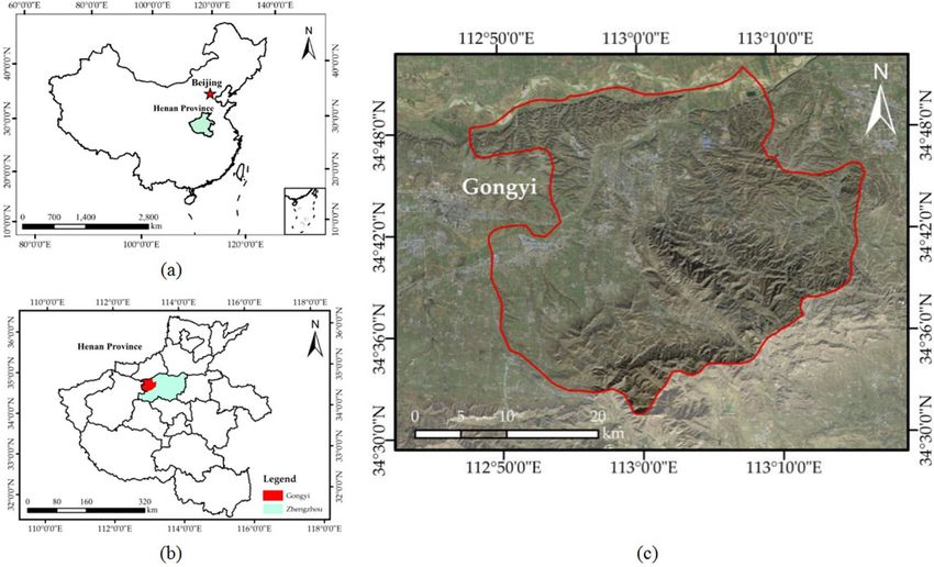
www.nature.com/scientificreports/
Figure 3. Socio-natural factors. (a) Elevation; (b) slope; (c) rainfall; (d) temperature; (e) solar radiation; (f)
air quality index; (g) soil type; (h) NDVI; and (i) land use types. The Figure is created using ArcGIS ver.10.3
(https://www.esri.com/).
Scientific Reports | (2021) 11:17549 | https://doi.org/10.1038/s41598-021-96625-9 5
Vol.:(0123456789)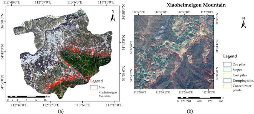
www.nature.com/scientificreports/
Figure 4. Methodological flowchart of the research process.
commonly used and best-performing classifiers because of its excellent generalization ability. The SVM optimi-
zation goal is to minimize the risk of the structure, rather than the least risk, thus reducing the data size and data
distribution requirements, which is helpful in the field of environmental assessment. However, an SVM is not
better than any other algorithm in any scenario because it is difficult and time consuming for an SVM to train
large amounts of data, so there are some limitations for a wide range of real-time evaluation analyses. At present,
SVMs have been well applied in the fields of time series analysis, regression analysis, cluster analysis, signal
processing, image classification, and control systems, but the application of SVMs in environmental assessment
has just started.
Training data sets, i.e., D = {(x1,y1)…,(xl,yl) }, where l is the sample size and D is the training set, are used to
estimate the regression function in the linear function s et36:
f (x, a) = ωx + b (1)
The SVM algorithm minimizes function (2) under constraint (3) using the principle of structural risk
minimization.
l
1
� ω, ξi+ , ξi− = (ω · ω) + c
+ −
(2)
ξi , ξi
2
i=1
yi − (ω · xi ) − b ≤ ξi+ + ε
(ω · xi ) + b − yi ≤ ξ − + ε
i
+
i = 1, 2, ..., l (3)
ξi ≥ 0
−
ξi ≥ 0
In this formula, c is the penalty coefficient, which determines a compromise between empirical risk error and
model complexity; ξi+ and ξi− are relaxation factors; ε is the allowable error; b is the offset; l is the number of train-
ing samples; and ω is the weight vector. By constructing the Lagrange function, the dual problem of the original
function is obtained, and the above problem eventually becomes a convex quadratic programming problem.
CART model. The CART model is a nonparametric nonlinear regression method proposed by Breiman
et al.37. The basic principle of the CART model is a binary decision tree structure formed by cyclic analysis of
training data sets composed of test variables and target variables. The CART algorithm uses the Gini index as the
criterion for selecting the best test variable. The Gini index is defined as follows:
J
p2 j/h
Gini Index = 1 − (4)
j
Scientific Reports | (2021) 11:17549 | https://doi.org/10.1038/s41598-021-96625-9 6
Vol:.(1234567890)www.nature.com/scientificreports/
Biological abundance Vegetation coverage Pollution loading
Index index index River density index Land stress index index
Weight (%) 0.35 0.25 0.15 0.15 0.10
Table 1. Weights of the evaluation indicators.
J
nj (h)
P j/h = , P j/h = 1 (5)
n(h) j
In this formula, a sample from the training sample set is randomly extracted, and when a test variable has a
value of h, the probability of belonging to the jth class is p(j/h); n
j(h) is the number of samples belonging to the
jth class when the test variable value is h in the training sample; n(h) is the number of samples in the training
sample whose test variable value is h; and j is the number of categories.
Learning samples are required to build and evaluate the CART decision tree before using the CART model
for prediction. The CART model uses the learning sample set of the following structure:
L := {X1 , X2 , . . . , Xm , Y } (6)
(7)
X1 := x11 , x12 , . . . , x1t1 , . . . , Xm := xm1 , xm2 , . . . , xmtn
(8)
Y := y1 , y2 , . . . , yk
X1–Xm are attribute vectors, and their attributes are continuous or discrete. Y is the label vector, and its attributes
can also be continuous or discrete. When Y is a continuous quantity value, it is a regression tree; when Y is a
discrete value, it is a classification tree.
The CART algorithm selects one attribute or a combination of multiple attributes from a plurality of input
attributes of the model as a splitting variable of the tree node and divides the test variable into branches; this
process is repeated to establish a sufficiently large classification tree. Then, the pruning algorithm is used to prune
the tree, and a series of nested classification trees are obtained. Finally, the series of classification trees are tested
with test data, and the optimal classification tree is selected. The CART algorithm can be used for classification
and regression, and it has considerable robustness and scalability in dealing with abnormal data. For example,
when certain monitoring data are missing or abnormal, this algorithm will not allow the outliers to damage the
final result. However, it is difficult for this algorithm to make predictions with continuous data38.
The C5.0 algorithm is also an algorithm in the decision tree model family and has certain similarities with
the CART algorithm. The growth process of the C5.0 decision tree uses the principle of the maximum informa-
tion gain rate for node selection and splitting point selection. The C5.0 model is very robust for missing data
and problematic fields and is easier to understand and explain than some other types of models39. However, the
calculation process of this algorithm is too complicated when calculating the information gain rate, and it is
prone to overfitting and decision tree bias.
Results
Technical criterion for ecosystem status evaluation. On March 3, 2015, the Ministry of Ecology and
Environment of the People’s Republic of China approved the "Technical Criterion for Ecosystem Status Evalua-
tion" as the national environmental protection standard. This standard is based on the former standards released
in 2006, and 48 relevant documents from 2006 to 2012 were searched to propose new standards and factor
weights based on actual utilization effects and expert guidance. The eco-environment assessment uses a compre-
hensive index (eco-environmental status index, EI) to reflect the overall state of the regional eco-environment.
The indicator system includes the biological abundance index, vegetation coverage index, river density index,
land stress index, and pollution loading index. These indexes reflect the abundance of organisms in the evaluated
area, the level of vegetation coverage, the abundance of water, the intensity of land stress, and the extent of the
pollution load. Each indicator was calculated according to its weight to obtain an eco-environment assessment
map (Table 1). All parameters involved in the calculation are derived from this standard.
The calculation of the eco-environment status is as follows:
EI = 0.35 ∗ biological abundance index + 0.25 ∗ vegetation coverage index
+ 0.15 ∗ river density index + 0.15 ∗ (1 − land stress index) (9)
+ 0.1 ∗ (1 − pollution loading index)
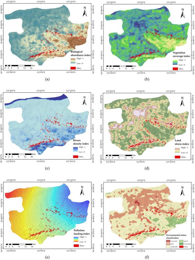
Biological abundance index. The biological abundance index refers to the number of certain organisms in this
area. The calculation method is as follows:
Biological abundance index = (BI + HQ)/2 (10)
Scientific Reports | (2021) 11:17549 | https://doi.org/10.1038/s41598-021-96625-9 7
Vol.:(0123456789)www.nature.com/scientificreports/
In this formula, BI is the biodiversity index and HQ is the habitat quality index. When the biodiversity index
does not have dynamic data updates, the change in the biological abundance index is equal to the change in the
HQ.
Biodiversity is a general term for the complexity of species and their genetic variation and ecosystems in space
over time. Biodiversity plays an important role in maintaining soil fertility, ensuring water quality, regulating the
climate, stabilizing the environment, and maintaining ecological balance.
The BI method is as follows:
BI = NPPmean ∗ Fpre ∗ Ftem ∗ (1 − Falt ) (11)
NPPmean is the net primary productivity. F pre is the annual average precipitation. F
tem is the temperature
parameter. Falt is the altitude parameter.
NPP refers to the amount of organic matter accumulated per unit area and unit time of green plants. NPP
is the remainder of the total amount of organic matter produced by photosynthesis after deducting autotrophic
respiration and is usually expressed as dry weight. In this study, the estimation of NPP was based on the absorbed
photosynthetically active radiation (APAR) and actual light-use efficiency (LUE) (ε) of the CASA ecosystem
model40. The CASA model is a process-based remote sensing model that couples ecosystem productivity and
soil carbon and nitrogen fluxes, driven by gridded global climate, radiation, soil, and remote sensing vegetation
index datasets41. The model can be expressed generally as follows:
NPP(x, t) = APAR(x, t) ∗ ε(x, t) (12)
The entire study area is divided into 11,303 pixels on a 30 * 30 m grid. x indicates the location of each pixel,
and t indicates time; the data were collected once a month. APAR(x,t) represents the photosynthetically active
radiation absorbed by pixel x in that month (gC * m−2* month−1). Ɛ(x, t) is LUE (gC * MJ−1) of the vegetation42.
Estimation of the fraction of APAR using RS data is based on the reflection characteristics of the vegetation
on the infrared and near-infrared bands. The value of APAR is determined by the effective radiation of the sun
and the absorption ratio of the vegetation to the effective photosynthetic radiation. The formula is as follows:
APAR(x, t) = SOL(x, t) ∗ FPAR(x, t) ∗ 0.5 (13)
where SOL(x,t) represents the total amount of solar radiation at pixel x in month t, FPAR(x,t) represents the
absorption ratio of the vegetation layer to the incident photosynthetically active radiation, and a constant of 0.5
indicates the ratio of the effective solar radiation that can be utilized by the vegetation to the total solar radiation.
Since there is a linear relationship between FPAR and NDVI within a certain range, this relationship can be
determined according to the maximum and minimum values of a certain vegetation type NDVI and the cor-
responding FPAR maximum and minimum values.
(NDVI(x, t) − NDVIi,min )
FPAR(x, t) = ∗ (FPARmax − FPARmin ) + FPARmin (14)
(NDVIi,max − NDVIi,min )
where NDVImax and N DVImin correspond to the NDVI maximum and minimum values of the ith planting type,
respectively. There is also a good linear relationship between FPAR and the simple ratio index (SR) of vegetation,
which is represented by the following formula:
(SR(x, t) − SRi,min )
FPAR(x, t) = ∗ (FPARmax − FPARmin ) + FPARmin (15)
(SRi,max − SRi,min )
where the values of FPARmin and F PARmax are independent of vegetation type and are 0.001 and 0.95, respectively;
SRi,max and SRi,min correspond to the 95% and 5% percentiles, respectively, of the ith NDVI. SR(x,t) is represented
by the following formula:
1 + NDVI(x, t)
SR(x, t) = (16)
1 − NDVI(x, t)
A comparison of the estimated results of FPAR-NDVI and FPAR-SR shows that the FPAR estimated by NDVI
is higher than the measured value, while the FPAR estimated by SR is lower than the measured value, but the error
is less than that estimated directly by NDVI. As a result, these two values can be combined, and their weighted
average value is taken as an estimate of the estimated FPAR, while ɑ means weight:
FPAR(x, t) = αFPARNDVI + (1 − α)FPARSR (17)
Light use efficiency (LUE) refers to the ratio of chemical energy contained in organic dry matter produced
per unit area over a certain period of time to the photosynthetically active radiation absorbed by plants projected
onto the same area at the same time. Different vegetation types and the same types of vegetation have different
light energy utilization rates in different living environments43. The differences are mainly due to the character-
istics of the vegetation itself, temperature, moisture, and s oil44. Vegetation has the highest utilization rate of light
energy under ideal conditions, but the maximum light energy utilization rate in the real environment is mainly
affected by temperature and moisture, which can be expressed as follows:
ε(x, t) = Tε1 (x, t) · Tε2 (x, t) · Wε (x, t) · εmax (18)
Scientific Reports | (2021) 11:17549 | https://doi.org/10.1038/s41598-021-96625-9 8
Vol:.(1234567890)www.nature.com/scientificreports/
Land use types Woodland Shrub Sparse woodland Grassland Water Construction land Arable land
εmax 0.638 0.429 0.475 0.542 0.542 0.542 0.542
Table 2. Maximum LUE rates of different land use types.
Figure 5. NPP calculation process.
where Tε1(x,t) and T ε2(x,t) represent the stress effects of low temperature and high temperature on light energy
utilization, respectively, W
ε(x,t) is the effect of water stress on the maximum light energy utilization under ideal
conditions, and εmax is the maximum light energy utilization under ideal conditions (gC * MJ−1). The maximum
solar energy utilization rate εmax varies depending on the vegetation type. In this study, the maximum light energy
utilization rate of different land use types simulated by an improved Carnegie-Ames-Stanford Approach (CASA)
model is used as the input parameter of light energy utilization in the CASA model (Table 2). The monthly
maximum light energy utilization rate is determined in three steps: first, calculate the APAR, temperature,
and water stress factors of all pixels; then, select the NPP measured data of the same time period in the study
area; finally, simulate the εmax of vegetation according to the principle of minimum error45. Figure 5 shows the
calculation process of NPP. The weight of each habitat type in the HQ is shown in Table 3. The weight value is
derived from the official document30. To facilitate the calculation, this paper normalizes the calculation results
from 0 to 1 (Fig. 6a).
Vegetation coverage index. The vegetation coverage index was obtained from the NDVI, which is a simple,
effective, and empirical measure of surface vegetation status. The vegetation index mainly describes the differ-
ence between the reflection of vegetation in the visible and near-infrared bands and the soil background. This
index also reduces the solar elevation angle and noise caused by the atmosphere and is thus the most widely
used and effective calculation method. Each vegetation index can be used to quantitatively describe the growth
of vegetation under certain conditions. The expression is as follows:
NIR − R
NDVI = (19)
NIR + R
where NIR and R are reflectance values in the near-infrared and red bands, respectively.
NDVI values are obtained by processing the RS images of the Landsat 8 satellite. This satellite is equipped
with an operational land imager (OLI) that includes nine bands with a spatial resolution of 30 m, including a
15-m panchromatic band. To facilitate the calculation, this paper normalizes the calculation results from 0 to
1 (Fig. 6b).
River density index. The river density index refers to the total length of rivers, lakes, and water resources in the
assessed area as a percentage of the assessed area, which is used to reflect the abundance of water in the assessed
area and is calculated as follows:
River density index = (Ariv ∗ river length/area + Alak ∗ water area/area
(20)
+Ares ∗amount of resources/area )/3
where Ariv is the normalization coefficient of river length, with a reference value of 84.3704, A
lak is the normali-
zation coefficient of the lake area, with a reference value of 591.7909, and Ares is the normalization coefficient
Scientific Reports | (2021) 11:17549 | https://doi.org/10.1038/s41598-021-96625-9 9
Vol.:(0123456789)www.nature.com/scientificreports/
Land use types Weights (%) Habitat type Weights (%)
Woodland 0.60
Woodland 0.35 Shrubbery 0.25
Sparse woodland and other woodland 0.15
High coverage grass 0.60
Grassland 0.21 Medium coverage grass 0.30
Low coverage grass 0.10
River 0.10
Lake 0.30
Water wetland 0.28
Beach wetland 0.50
Permanent glacier snow 0.10
Paddy field 0.60
Arable land 0.11
Rainfed cropland 0.40
Urban construction land 0.30
Construction land 0.04 Rural settlement 0.40
Other construction land 0.30
Sandy land 0.20
Saline-alkali land 0.30
Unutilized land 0.01 Bare land 0.20
Bare rock gravel 0.20
Other unused land 0.10
Table 3. Weight of each habitat type in the HQ.
of water resources, with a reference value of 86.387. Finally, the calculation results were normalized from 0 to
1 (Fig. 6c).
Land stress index. The land stress index is the degree to which the land quality in the assessment area is under
stress. The weight of the land stress index evaluation is shown in Table 4.
The calculation method is as follows:
Land stress index = Aero ∗ (0.4 ∗ severe erosion area + 0.2 ∗ moderate erosion area
(21)
+0.2 ∗ construction land area + 0.2 ∗ other land stress area)/area
where Aero is the normalization coefficient of the land stress index, with a reference value of 236.0436. According
to the “Classification criteria for soil erosion”46, the influencing factors of soil erosion, vegetation, soil texture,
landform, and precipitation are ranked according to importance. In the calculation of the land stress index, all
the land is divided into three categories, in which the weight of severe erosion is 0.4, the weight of non-erosion
is 0, and the other erosion types such as moderate erosion and construction land are 0.2. The areas with severe
erosion include vegetation coverage less than 30% and areas of soil erosion greater than 3.7 mm/a due to human
activities. These areas are generally developed on highly erosive-sensitive soils. Cinnamon soil and loess soil in
the study area are highly erosive-sensitive soils. Therefore, the industrial and mining areas of cinnamon and loess
soil types are regarded as severe erosion areas. Areas with vegetation coverage greater than 50% are non-eroded
areas, so water bodies and woodlands are divided into non-erodible areas. All areas except these two types have
a weight of 0.2. Finally, the calculation results were normalized from 0 to 1 (Fig. 6d).
Pollution loading index. The pollution loading index refers to the load of pollutants in a certain area or an
environmental element. In this study, the AQI was used to calculate the pollution loading index, and the results
were normalized from 0 to 1 (Fig. 6e).
The eco-environmental evaluation score was calculated based on the national environmental protection
standard according to the weight of each indicator (Fig. 6f).
Improved evaluation system and intelligent evaluation model. Improved evaluation sys-
tem. Considering that the evaluation factors in the national environmental protection standards are applicable
to ordinary areas, areas affected by mines should have more evaluation factors than those in the standards.
Thus, an improved evaluation system was proposed. The improved evaluation system has added factors that
affect the environment of the mine based on the factors of the original system. The impact of the mine on the
environment is reflected in the pollution of the atmosphere, such as dust from open pits and industrial waste
from concentrators; the occupation of land by solid waste, such as ore piles and coal piles; soil pollution, such as
the diffusion of heavy metals from coal piles, coal mine concentrator plants, and mines; and the increased likeli-
hood of geological disasters, such as collapse caused by underground mining, spontaneous coal combustion and
landslides caused by open-pit mining surfaces. Therefore, the improved evaluation system adds an air pollution
Scientific Reports | (2021) 11:17549 | https://doi.org/10.1038/s41598-021-96625-9 10
Vol:.(1234567890)www.nature.com/scientificreports/
Figure 6. Eco-environment assessment indexes and evaluation rating map (the first quarter was
used as an example). (a) Biological abundance index; (b) vegetation coverage index; (c) river density
index; (d) land stress index; (e) pollution loading index; and (f) environmental status classification.
The Figure is created using ArcGIS ver.10.3 (https://www.esri.com/).
Scientific Reports | (2021) 11:17549 | https://doi.org/10.1038/s41598-021-96625-9 11
Vol.:(0123456789)www.nature.com/scientificreports/
Type Severe erosion Moderate erosion Construction land Other land stress
Weight (%) 0.4 0.2 0.2 0.2
Table 4. Weight of the land stress index evaluation.
range, a solid waste area, a geologic hazard range, and a metallic and non-metallic mine soil pollution buffer to
the national environmental protection standards.
The area of air pollution in mining areas is generally near open pits and concentrator plants. Therefore, the air
pollution range was selected within 50 m around the open pits and the concentrator plants. Due to the dilution
and dispersion of the air itself, an estimate of the pollution is the reciprocal of the wind speed (Fig. 7a).
Mine solid waste pollution includes a large amount of waste rock from open-pit mining and pit mining,
coal gangue produced by coal mining, tailings from beneficiation and slag from smelting. These solid wastes
are generally piled up near the mining area. They not only occupy large areas of land and induce geological
disasters such as landslides and mudslides but also cause chemical pollution, spontaneous combustion, and
radiation from radioactive materials due to long-term stacking. This may affect the health and safety of humans
and other biological organisms. The scope of the solid waste area is determined by the ore piles, coal piles, and
dumping sites (Fig. 7b).
Mine geological disasters are caused by a large number of mining wells and rock and soil deformation, as well
as serious changes in the geological, hydrogeological, and natural environments of the mining area, endangering
human life and property and destroying mining engineering equipment and mining resources. In this study, the
geologic hazard range consists of areas with underground mining stopes and coal piles (Fig. 7c).
After the pollutants generated by the mining operation enter the soil, physical and mechanical absorption,
retention, colloidal physicochemical adsorption, chemical precipitation, bioabsorption, etc. of the suspended
pollutants through the soil continue to accumulate in the upper soil. When pollutants reach a certain maximum,
they cause deterioration of the soil composition, cycle, properties, and functions and begin to accumulate in
plants, which affects the normal growth and development of plants, decreases crop yield and quality, and ulti-
mately affects human health. Metallic and non-metallic minerals have different effects on soil pollution. The
pollution of soil by non-metallic minerals mainly occurs in coal mines and coal piles, and the buffer zone is
centred on the coal mines and coal piles. Coal production activities can cause heavy metals in coal piles to enter
the soil and cause pollution. Due to different types of heavy metals, the range of soil contamination is d ifferent47.
Combining the non-metallic mineral industrial squares and coal mine-based non-metallic minerals around the
heavy metal soil pollution range, the buffers are graded at 30, 200, and 1000 m (Fig. 7d1)43. The metal mines
in Gongyi are mainly aluminium ore and iron ore. Referencing the spread range of heavy metal pollution in
the soil of aluminium ore and iron ore mines48–51, the buffers are graded at 50, 100, 300, and 500 m (Fig. 7d2).
The four new elements in the improved evaluation system are normalized from 0 to 1 during the calculation.
Intelligent evaluation model. Artificial neural networks, decision trees, and SVMs were calculated using IBM
SPSS Modeler software to find an intelligent model suitable for environmental assessment of the mine in the
study area. Then, several models with high evaluation accuracy were selected. The SVM, CART, and C5.0 models
were chosen for further comparison. The sampling points were selected randomly; 700 sampling points were
selected from the area away from the mining area; 100 sampling points were selected from the mining area after
random sampling by mine type, and these points were used as training samples. Non-mining evaluation scores
were based on the national environmental protection standard, while the mining area scores were based on field
investigation. In the field investigation, preliminary scoring of the sampling points was conducted according to
mining type, mining intensity, air quality, and surrounding environment. Then, a photo of the field was taken at
every sampling point in the mine, and experts were invited to further score the area according to the photo. This
score is the relative score obtained by referencing the national environmental protection standard.
The index layers of the training samples were used as input, and the scores were used as the output to train
the machine learning models. The trained models were applied to the entire study area, and all points except
the training sample points were used for verification. After further comparison with SVM, CART, and C5.0,
the evaluation accuracy rates of the three methods in the mining area and non-mining area were obtained. In
the non-mining area, the model evaluation results of various land use types were compared with the national
environmental protection standards. The accuracy in various land use types is shown in Table 5. In the mining
area, the model evaluation score is compared with the score from the experts, and the obtained accuracy table
is shown in Table 6.
In non-mining areas, the accuracy of the SVM model is significantly better than that of the other two methods.
However, in the mining area, the accuracy of the CART model is higher. Therefore, the SVM model was used to
evaluate the area away from the mine, and the CART model was used to evaluate the mining area. The evaluation
results of these two models were combined to obtain the evaluation map of the entire study area.
Discussion
Comparing the former evaluation results of the first season to the evaluation results by the improved system
shows that the overall difference in the new results is more obvious and that the pollution of the mining area is
increased. The mountainous area in the southeast is unexplored forestland and is far away from the mining area
and the city. Thus, the vegetation coverage is high, and logically, the eco-environmental quality should be the best.
However, the official evaluation results do not prominently reflect this information, but the improved evaluation
Scientific Reports | (2021) 11:17549 | https://doi.org/10.1038/s41598-021-96625-9 12
Vol:.(1234567890)www.nature.com/scientificreports/
Figure 7. New factors in the improved evaluation system. (a) Air pollution range; (b) solid waste area; (c)
geological hazard range; (d1) non-metallic mine soil pollution buffer; and (d2) metal mine soil pollution buffer.
The Figure is created using ArcGIS ver.10.3 (https://www.esri.com/).
Scientific Reports | (2021) 11:17549 | https://doi.org/10.1038/s41598-021-96625-9 13
Vol.:(0123456789)www.nature.com/scientificreports/
Algorithm
Land use types SVM (%) CART (%) C5.0 (%)
Mining lease 98.37 99.08 98.06
Residential land 71.57 80.15 78.45
Scenic spot 100.00 100.00 99.78
Road 99.02 97.89 97.85
Woodland 79.74 78.40 81.47
Garden 99.67 99.17 99.78
Arable land 68.63 66.36 65.73
Water 94.12 91.82 91.16
Grassland 90.85 88.05 89.22
Other land 98.04 99.08 98.49
Totals 94.80 84.55 91.90
Table 5. Accuracy of each algorithm in various land use types in non-mining areas.
Algorithm SVM (%) CART (%) C5.0 (%)
Accuracy 82.50 89.36 85.62
Table 6. Accuracy of each algorithm in the mining area.
results of the area show good indications of an excellent environment. The difference in the evaluation results of
the southwestern, northern, and central-eastern regions of the improved system is larger than that of the former
systems, which is not as consistent as the results of large-area regional evaluations. Taking the northern region
as an example, as a region containing different vegetation indexes, air pollution values, meteorological factors,
and a large variety of land types, such as water bodies, construction land, and forestland, the results from the
official evaluation methods are very similar, while the improved results can reflect the role of various factors in
this region. This comparison further illustrates the accuracy and practicality of the improved evaluation system.
In addition, the meteorological data were divided into four seasons. March to May 2016 was defined as the
first season (spring), June to August 2016 was defined as the second season (summer), September to November
2016 was defined as the third season (autumn), and December 2016 to February 2017 was defined as the fourth
season (winter). The final composite model was used to calculate the geo-environmental assessment scores, and
then, the eco-environment assessment map of the mining area in Gongyi was generated (Fig. 8). The results
of the eco-environment assessment of the mining area were divided into five levels: very bad, bad, moder-
ate, good, and very good. The following conclusions were obtained from the map: (1) the areas with very bad
eco-environmental assessments are first distributed in the hilly development zone in the northwestern part of
the central area, followed by the mining area in the southeastern mountainous area; (2) in addition to central
residential areas and key mining areas, the moderate level of residential concentration and the small mining
areas are more susceptible to climatic conditions, and such effects usually have a certain seasonality; (3) areas
covered by water, such as rivers, do not necessarily have a good eco-environment; and (4) in the mountainous
area of the southwest corner, except for the poor environment in the mining area, the seasonal changes in the
surrounding areas are particularly obvious.
Table 7 shows the Pearson correlation coefficient values between the evaluation maps and the evaluation
indexes, and the following conclusions can be obtained: (1) in spring, the quality of the eco-environment is
mainly determined by the vegetation coverage index, followed by the biological abundance index, because the
vegetation develops at the turn between winter and spring, so the impact of vegetation on the environment is
highlighted. The relationship between this evaluation and the pollution loading index is different from the other
three seasons, indicating that the changes in the AQI in the spring have less impact on the eco-environment. In
this season, the area of the mining region with poor environmental quality is particularly large, which means that
in the spring, the environmental quality is most affected by mining activities. (2) In summer, the impact of the
vegetation coverage index and biological abundance index on the eco-environment is still the most prominent,
but the impact of the vegetation coverage index in summer is much weaker than that in spring. In the mountains
of the south and southwest, the environmental quality is particularly poor compared to the other three seasons,
which is related to the strong negative effect of the land stress index and air pollution range. (3) In autumn, the
negative effects of the land stress index and pollution loading index are more pronounced, and the negative
correlation with the geologic hazard range also increases, while the river density index that should be positively
correlated becomes abnormal, which leads to low environmental quality in the entire northern region in autumn.
The environmental quality of the southern mountains in autumn is better than that in the other three seasons.
(4) In winter, the biological abundance index has little impact on environmental quality, and the environmental
quality of the surrounding areas of the key mining areas is significantly different from that inside the mining area,
which means that the mining area has little impact on the surrounding environment. The river density index
Scientific Reports | (2021) 11:17549 | https://doi.org/10.1038/s41598-021-96625-9 14
Vol:.(1234567890)www.nature.com/scientificreports/
Figure 8. Eco-environment assessment maps of the mining area in Gongyi. (a) Maps of spring; (b) maps of
summer; (c) maps of autumn; and (d) maps of winter. The Figure is created using ArcGIS ver.10.3 (https://www.
esri.com/).
Seasons
Indexes Spring Summer Autumn Winter
Biological abundance index 0.472 0.419 0.389 − 0.044
Vegetation coverage index 0.714 0.571 0.425 0.323
River density index 0.093 0.091 − 0.016 0.268
Land stress index − 0.293 − 0.302 − 0.357 − 0.353
Pollution loading index 0.142 − 0.244 − 0.376 − 0.366
Air pollution range − 0.088 − 0.108 − 0.094 − 0.110
Solid waste area − 0.197 − 0.214 − 0.232 − 0.244
Geologic hazard range − 0.125 − 0.133 − 0.156 − 0.150
Mine soil pollution buffer − 0.134 − 0.112 − 0.093 − 0.110
Table 7. Pearson correlation coefficient values between the evaluation results and evaluation indexes.
Scientific Reports | (2021) 11:17549 | https://doi.org/10.1038/s41598-021-96625-9 15
Vol.:(0123456789)www.nature.com/scientificreports/
has significantly increased control over the environmental quality, so the environmental quality of the northern
river covered area is obviously good.
The indicator layers in the national standard document referenced in the system are feasible for evaluating
the environment of a normal area. The advantages are consistent with the integration of various factors of the
classic models for evaluation, such as CIM. After considering the impact of the mine region, the combination
with machine learning is more practical and objective than classic models.
Conclusion
This paper uses national standard documents and machine learning methods to assess the ecological environment
of mines. Environmental assessment maps for the entire study area and a practical environmental assessment
model of mining areas were generated. The first advantage lies in the use of high spatial resolution RS images for
mine interpretation and field sampling surveys to improve the interpretation results. This process is not limited
to only traditional field investigations for interpretation of the mining area but also uses RS to save time and
effort. Second, in terms of factor selection, this process utilizes the factors of national standards and increases
the factors related to mines, adding various considerations. This method combines relevant factor layers and
machine learning for environmental assessment. This strategy can be used in other regions of the world to obtain
appropriate composite algorithms based on different environmental characteristics. Compared with other classic
methods that use specific rules or artificially determined factor weights, such as AHP, machine learning methods
are more accurate and reliable, and system flexibility and scalability are improved. However, because of the scale
limitation of some specific factors, some of the factors involved in the calculation cannot be determined according
to the actual situation. Nevertheless, with the addition of more comprehensive factors, a higher accuracy of the
assessment model can be achieved. These problems still deserve further study. With the optimization of machine
learning algorithms, algorithms based on subjective experience will reveal greater limitations, and consequently,
an increasing number of machine learning algorithms will be used in the field of environmental assessment.
Received: 26 December 2020; Accepted: 5 August 2021
References
1. Lukichev, S. V. & Nagovitsin, O. V. Information support of mineral mining and exploitation in the Khibiny Mountains area. J. Min.
Sci. 48(6), 1025–1030 (2012).
2. Liu, H. R., Chen, S. Q. & Li, S. Fuzzy evaluation of the impact of the open-pit limestone mining on geological environment. Adv.
Mater. Res. 1073–1076, 454–459 (2015).
3. Cheng, Y. P. et al. The controlling effect of thick-hard igneous rock on pressure relief gas; drainage and dynamic disasters in outburst
coal seams. Nat. Hazards 66(2), 1221–1241 (2013).
4. Tao, J. L. & Chen, W. J. Influence of open pit mining on geological environment and its prevention and control countermeasures.
Inner Mongolia Coal Econ. 06, 41–42 (2018).
5. Xu, Z. Y. Discussion on geological environment restoration and comprehensive control of open-pit mines in Gongyi City. Environ.
Dev. 31(06), 247–247 (2019).
6. Liu, D., Ma, J., Sun, Y. & Li, Y. Spatial distribution of soil magnetic susceptibility and correlation with heavy metal pollution in
Kaifeng City, China. CATENA 139, 53–60 (2016).
7. Zhao, Y. et al. Research on heavy metal level and co-occurrence network in typical ecological fragile area. J. Environ. Health Sci.
Eng. 19, 531–540 (2021).
8. Kope, A. et al. Application of remote sensing, gis and machine learning with geographically weighted regression in assessing the
impact of hard coal mining on the natural environment. Sustainability. 12(22), 9338 (2020).
9. Rinaldi, L. et al. Geographical information systems and remote sensing technologies in parasitological epidemiology. Parassitologia
46(1–2), 71–74 (2004).
10. Xu, J., Zhao, H., Yin, P., Wu, L. & Li, G. Landscape ecological quality assessment and its dynamic change in coal mining area: A
case study of peixian. Environ. Earth Sci. 78(24), 1–13 (2019).
11. Khalil, A., Hanich, L., Hakkou, R. & Lepage, M. Gis-based environmental database for assessing the mine pollution: A case study
of an abandoned mine site in Morocco. J. Geochem. Explor. 144(SI), 468–477 (2014).
12. Yan, C., Liu, R., Liu, S., & Wu, I. Study of remote sensing index indicators about the mine environment evaluation. In Proceedings.
2004 IEEE International Geoscience and Remote Sensing Symposium. IGARSS ’04, Vol.1, 581 (2004).
13. Xie, Q., Ni, J. Q. & Su, Z. Fuzzy comprehensive evaluation of multiple environmental factors for swine building assessment and
control. J. Hazard. Mater. 340, 463–471 (2017).
14. Qiu, Z. Y., Liang, W., Wang, X., Lin, Y. & Zhang, M. Study on quantitative risk assessment model of the third party damage for
natural gas pipelines based on fuzzy comprehensive assessment. In Journal of Physics: Conference Series, Vol. 842, no. 1 (2017).
15. Sahoo, S., Dhar, A. & Kar, A. Environmental vulnerability assessment using grey analytic hierarchy process based model. Environ.
Impact Assess. Rev. 56, 145–154 (2016).
16. He, F., Gu, L., Wang, T. & Zhang, Z. The synthetic geo-eco-environmental evaluation of a coastal coal-mining city using spati-
otemporal big data: A case study in Longkou, China. J. Clean. Prod. 142(SI), 854–866 (2016).
17. Zhang, W., Wang, W. & Wang, S. Environmental performance evaluation of implementing ems (iso 14001) in the coating industry:
Case study of a Shanghai coating firm. J. Clean. Prod. 64(2), 205–217 (2014).
18. Wang, X., Li, G., & You, B. Evaluating the quality of mine environment based on rank correlation analysis. In International Confer-
ence on Remote Sensing, Environment and Transportation Engineering, 4952–4955 (IEEE, 2011).
19. Ranjan, A. K., Sahoo, D. & Gorai, A. K. Quantitative assessment of landscape transformation due to coal mining activity using
earth observation satellite data in Jharsuguda coal mining region, Odisha, India. Environ. Dev. Sustain. 23(3), 4484–4499 (2020).
20. Shang, M. J., Zhou, Z. F., Wang, X. Y., Huang, D. H. & Zhang, S. S. Evaluation of soil environmental quality in karst mountain
area based on support vector machine: A case study of a tea plantation in northern Guizhou. Carsologica Sinica. 37(04), 575–583
(2018).
21. Li, D. et al. Application of BP neural network and SVM in mine environmental assessment. Arid Land Geogr. 38(01), 128–134
(2015).
22. Cheng, W., Zhang, X., Wang, K. & Dai, X. L. Integrating classification and regression tree (CART) with GIS for assessment of heavy
metals pollution. Environ. Monit. Assess. 158(1–4), 419–431 (2009).
Scientific Reports | (2021) 11:17549 | https://doi.org/10.1038/s41598-021-96625-9 16
Vol:.(1234567890)You can also read