Simulations Approaching Data: Cortical Slow Waves in Inferred Models of the Whole Hemisphere of Mouse
←
→
Page content transcription
If your browser does not render page correctly, please read the page content below
Simulations Approaching Data: Cortical Slow Waves in Inferred
                                                         Models of the Whole Hemisphere of Mouse
                                             Cristiano Capone1 , Chiara De Luca1, 5 , Giulia De Bonis1 , Elena Pastorelli1 , Anna Letizia
                                             Allegra Mascaro2,3 , Francesco Resta2 , Francesco Pavone2,4 , and Pier Stanislao Paolucci1
                                                                                     1
                                                                                INFN, Sezione di Roma
arXiv:2104.07445v1 [q-bio.NC] 15 Apr 2021

                                                                                 2
                                                                                   LENS, Firenze, Italy
                                                                                      3
                                                                                        CNR, Italy
                                                                 4
                                                                   University of Florence, Physics Department, Italy
                                                     5
                                                       PhD Program in Behavioural Neuroscience, “Sapienza” University of Rome

                                                                                           April 16, 2021

                                            Abstract
                                            Recent enhancements in neuroscience, like the development of new and powerful recording techniques of
                                            the brain activity combined with the increasing anatomical knowledge provided by atlases and the growing
                                            understanding of neuromodulation principles, allow to study the brain at a whole new level, paving the way
                                            to the creation of extremely detailed effective network models directly from observed data. Leveraging the
                                            advantages of this integrated approach, we propose a method to infer models capable of reproducing the
                                            complex spatio-temporal dynamics of the slow waves observed in the experimental recordings of the cortical
                                            hemisphere of a mouse under anesthesia. To reliably claim the good match between data and simulations,
                                            we implemented a versatile ensemble of analysis tools, applicable to both experimental and simulated data
                                            and capable to identify and quantify the spatio-temporal propagation of waves across the cortex. In order to
                                            reproduce the observed slow wave dynamics, we introduced an inference procedure composed of two steps:
                                            the inner and the outer loop. In the inner loop the parameters of a mean-field model are optimized by
                                            likelihood maximization, exploiting the anatomical knowledge to define connectivity priors. The outer loop
                                            explores “external” parameters, seeking for an optimal match between the simulation outcome and the data,
                                            relying on observables (speed, directions and frequency of the waves) apt for the characterization of cortical
                                            slow waves; the outer loop includes a periodic neuro-modulation for a better reproduction of the experimental
                                            recordings. We show that our model is capable to reproduce most of the features of the non-stationary and
                                            non-linear dynamics displayed by the biological network. Also, the proposed method allows to infer which
                                            are the relevant modifications of parameters when the brain state changes, e.g. according to anesthesia levels.

                                            Introduction
                                            In the last decade, large-scale optical imaging coupled with fluorescent activity indicators have provided new
                                            insight on the study of the brain activity patterns [1, 21, 10, 40, 39, 16, 48, 45, 49]. The main tools currently
                                            employed to investigate neuronal activity at the mesoscale are Voltage Sensitive Dyes (VSDs) and Genetically
                                            Encoded Calcium Indicators (GECIs). Although there are a few studies that exploit the VSDs to explore
                                            the dynamics of cortical traveling waves during anesthesia [1, 39], the use of genetically encoded proteins
                                            presents important advantages. Indeed, GECIs are less invasive compared to synthetic dyes, they allow
                                            repeated measures on the same subject and – more important – can be targeted to specific cell populations.
                                            GECIs are indirect reporter of neuronal activity by changing their relative fluorescence following the activity-
                                            dependent fluctuations in calcium concentration [28, 20], and the usage of GECI to map spontaneous network

                                                                                                   1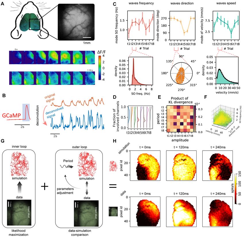
activity has recently supplied important information about the spatio-temporal features of slow wave activity
[48, 45]. Here we considered experimental recordings obtained from a genetically-modified mouse with the
GCaMP6f protein, a widely used GECI characterized by a very high sensitivity and a fast dynamic response
[10]. Despite the lower temporal resolution compared to state-of-the-art electrophysiological methods, the
imaging approach that combines calcium indicators with wide-field microscopy increases both the spatial
resolution and the specificity of the recorded neuronal population, and thus appears to be appropriate for
the objective we set of modelling large-scale network dynamics.
     Indeed, such a rich and detailed picture of the cortical activity allows for a deeper investigation of the
ongoing phenomena, and the first step toward the construction of data-constrained simulations is to explore
and characterize the slow wave dynamics displayed by the cortex of the mouse under anesthesia.
     This was achieved by developing an analysis procedure able to extract relevant observables, such as the
distributions of frequency of occurrence, speed and direction of propagation of the detected slow waves. The
set of analysis tool is flexible enough to be applied also to simulations, allowing a direct comparison between
the model and the experiment.
     The building of dynamic models requires to embody in a mathematical form the causal relationships
between variables deemed essential to describe the system of interest; of course, the value of the model is
measured both by its ability to match observations and by its predictive power.
     The classical approach to this problem is constructive: parameters appearing in the model are assigned
through a mix of insight from knowledge about the main architectural characteristics of the system to be
modeled, experimental observations and trial-and-error iterations. A more recent approach is to infer the
model parameters by maximizing some objective function, e.g. likelihood, entropy, or similarity defined
through some specific observable (e.g. functional connectivity). Following this route, a small number of
models have been able to reproduce the complexity of the dynamics observed from one single recording, and
most of them are focused on the resting state recorded through fMRI and on the reproduction of its functional
connectivity[2]. In [3] the temporal and spatial features of bursts propagation are accurately reproduced,
but on a simpler biological system, a culture of cortical neurons recorded with a 60 electrodes array. In this
work we address the complexity of the biological system, aiming at reproducing the dynamics observed in
the whole cortical hemisphere of a mouse with a high number of recording sites displaying non-trivial slow
waves propagation patterns. Indeed, each frame in the raw imaging dataset is 10000 pixels at 50µm × 50µm
spatial resolution; the selection of the cortical region of interest and a spatial coarse-graining step reduces
the number of recording and modeling sites down to 1400 pixels with spatial resolution of 100µm × 100µm,
still a number of channels larger than what usually accessed through wide-field electrophysiology.
     A major difficulty in assessing the goodness of the inferred model is the impossibility to directly com-
pare the parameters of the model with the elements of the biological system, that are usually unknown in
their entirety. To overcome this distance between experimental probing and mathematical description, our
approach is to consider the spontaneous activity as a testing ground to assess whether the inferred model
does capture the essential features of the biological system.
     The large number of elements in the system together with the fact that we relied on datasets of short-time
duration (8 recordings lasting 40s each), makes important the inclusion of good priors, since the resulting
inferred system might be under determined.
     A possible approach could be to make use of Structural Connectivity (SC) and Functional Connectivity
(FC) atlases that, however, are affected by degeneracy, individuality and, for the mouse, the typical need of
post-mortem processing [42, 27, 25].
     Instead, in our approach we exploited a minimal amount of generic anatomical knowledge (the exponential
decay characterizing the lateral connectivity [38], and the evidence about the suppression of inter-areal
excitatory connectivity during the expression of cortical slow waves [31] while lateral connectivity is preserved)
to set up the connectivity priors, introduced in the model as elliptical exponentially decaying connectivity
kernels. The introduction of such priors has also the beneficial effect of reducing the dependence of the
computational needs of the inference procedure on the number N of cortical pixels/populations in the system,
from O(N 2 ) down to O(N ).
     One common problem in inferring a model is that it is possible to constrain only some of the observables,
usually the average activity and the correlations between different sites [37, 5]. However it remains difficult to
constrain other aspects of the spontaneous generated dynamics [35], e.g. the shape of the traveling wavefronts

                                                        2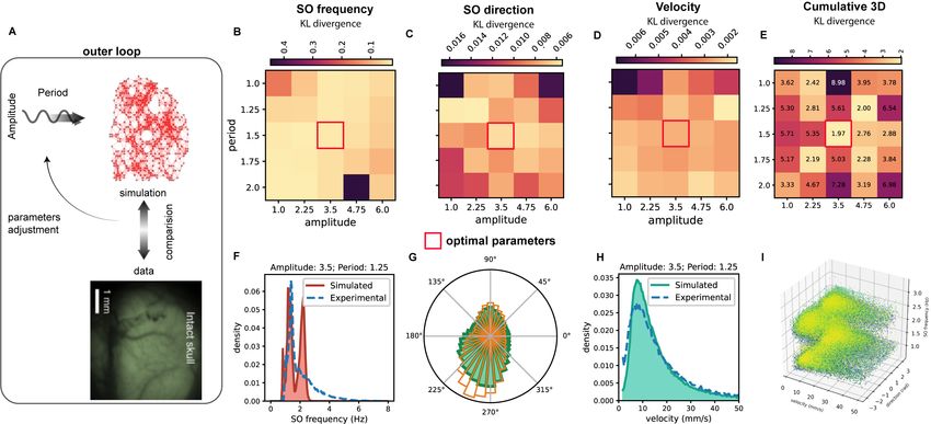
and the frequency of slow waves. Aware of this issue, we propose a two-steps approach that we name inner
loop and outer loop. In the inner loop, the model parameters are optimized by maximizing the likelihood of
reproducing the dynamics displayed by the experimental data at the following time step. In the outer loop,
the outcome of the simulation and the experimental data are compared through specific observables based
on the statistics of the whole time course of the spontaneously generated dynamics. Parameters are adjusted
to maximize the similarity between the original dynamics and the one of the generative model. Here we find
that the outer loop suggested that to ensure an optimal match between data and simulations it is necessary
to include an acethylcolinic neuro-modulation term [18] in the model which influences the excitability of
the network along the simulation time-course. The following Results section, presents the main elements of
this work, with further details presented in the Methods section. Finally, the Discussion section illustrates
limitations and potentials of the approach we introduced, in particular in relation with both the theoretical
framing and the experimental and modeling perspectives.

Results
Summary
The main objective of this section is to introduce and illustrate the summary Fig.1; please refer to the
following sub-sections and the Methods section for details.
     The aim of this work is to reproduce in a data-constrained simulation the activity recorded from a
large portion of the mouse cortex. We considered signal collected from the right hemisphere of a mouse,
anaesthetized with a mix of Ketamine and Xylazine. The activity is recorded through wide-field calcium
imaging (GCaMP6f indicator), see Fig.1A–top. In this anesthetized state, the cortex displays the occurrence
of slow waves (from ' 0.25Hz to ' 5Hz, i.e. covering a frequency range that corresponds to the full δ
frequency band and extends a little toward higher frequencies). The waves travel across different portions of
the cortical surface, exhibiting a variety of spatio-temporal patterns.
     Fig.1A–bottom reports a few frames of the luminosity signal displaying slow waves that are travelling
across the cortical tissue.
     The optical signal is highly informative about the activity of excitatory neurons, however the GCaMP6f
indicator, despite it is “fast” compared to other indicators, has a slow response in time if compared to the
time scale of the spiking activity of the cells, that is the target of the simulation (see Fig.1B–left). The
impact on the observed experimental signature can be described as a convolution with a low-pass transfer
function, resulting in a recorded luminosity that exhibits a peak after about 200ms from the onset of the
spike, and a long tailed decay [10]. To take into account this effect, we decided to perform a deconvolution of
the luminosity signal (Fig.1B–top), to better estimate the firing rate of the population of excitatory neurons,
i.e. the multi-unit activity, recorded by each single pixel (see Fig.1B–bottom).
     We considered 8 consecutive acquisitions (each one lasting 40s) collected from a single mouse subject,
recordings are named tn ∈ {t1, t2, ...t8} hereafter. For each acquisition, we characterized the properties
of the wave propagation. In Fig.1C–top the average frequency, speed, and direction of the waves in the
8 recordings are reported, to illustrate that the dynamics expressed in the different acquisitions is non-
stationary, and dynamic properties change in time. The distribution of frequencies, speeds, and directions
considering together t2 and t3 are reported in Fig.1C–bottom. For our modeling purposes in a data-driven
approach, we chose the two consecutive recordings t2 and t3, since: 1) according to the set of local observables
we defined (frequency, direction and speed) they manifest similar average behaviour (see Fig.1C-top); 2) they
express waves whose frequencies, directions and velocities are well in agreement with what expected from well-
expressed cortical slow-waves (see Fig.1C-bottom); 3) looking at Fig.1D, the t2 and t3 acquisitions express
waves that involve a relevant fraction of the cortex (in contrast e.g. to t4 and t6); 4) the Kullback-Leibler
divergence between t2 and t3 is lower than that computed for other acquisition segments (see Fig.1E, further
clarified by Fig.2); 5) they are consecutive in time (t8 appears to express a regime much similar to t3 but it is
not contiguous in time, a minor problem that we decided not to face in this work). Finally, confirming point
2) in the above list, the richness and compatibility with well expressed slow-wave of t2 and t3 is captured by
the 3D view of the full collection of their experimental local observations Fig.1F.
     We propose a 2-step inference method. In the first step, the inner loop, the parameters of the model

                                                       3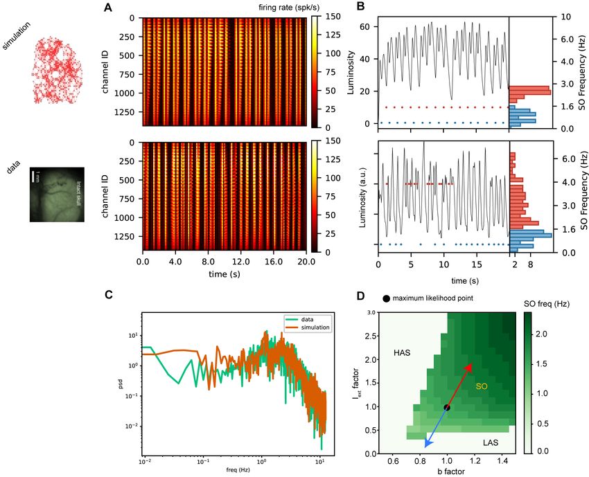
Figure 1: Experimental Setup and Model building. A. (top) The cortical activity of the right hemi-
sphere of a mouse (under ketamine anesthesia) is recorded through wide-field calcium imaging (GCaMP6f
indicator). (bottom) Consecutive frames of the luminosity signal displaying traveling slow waves across the
cortical tissue. B. The calcium indicator has a slow response in time (top). Applying a proper deconvolution
function (left, which is fitted from the single spike response [24, 10]) it is possible to estimate a good proxy
for the average activity for the local population of excitatory neurons recorded by a single pixel (bottom). C.
(top) Average frequency, speed, and direction of the waves in 8 consecutive recordings. (bottom) Distribu-
tions of frequencies, speeds, and directions for 2 out of the 8 recordings. D. Histogram of the fraction of the
hemisphere involved in the wavefront over all the waves for each recording. E. Kullback-Leibler divergence
between recordings, evaluated on the distributions defined in panel C. F. Each point represents one pixel,
each color represents a different wave. The three coordinates are speed, direction and frequency. G. Model
inference scheme, composed of an inner loop (likelihood maximization) and an outer loop (seeking for hyper-
parameters granting the best match by comparing simulations and data). H. 3 frames from the simulation
(top) and 3 frames from the data to show the similarities in SW propagation.

                                                       4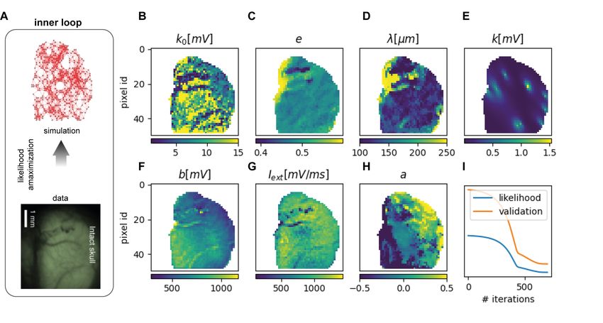
are inferred through likelihood maximization, Fig.1E–left, exploiting a set of known, but generic, anatomical
connectivity priors [38] and assuming that mechanisms of suppression of long-range connectivity are in action
during the expression of global slow waves[31]. Such anatomical priors have been introduced figuring that
the probability of connection among neural populations followed the shape of elliptical kernels exponentially
decaying with the distance. For each pixel, the inference has to identify the best local values for the parameters
of such connectivity kernel. In addition, for each acquisition period tn ∈ {t1, .., , t8} it identifies the best
local values (i.e. for each spatial location) for a neuro-modulated fatigue and for the external current. In
the second step, the outer loop, we seek for hyper-parameters granting the best match of the model with the
experiment by comparing simulations and data, Fig.1E-right. This second steps exploits acquired knowledge
about neuro-modulation mechanisms in action during cortical slow wave expression and a way to implement
these effects [18].
Finally, in Fig.1F, we provide a first preview of the fidelity of our simulations by reporting 3 frames
from the simulation (top) and 3 frames from the data. This example shows similarities in the slow wave
propagation: the origin of the wave, the wave extension and the activity are comparable and also the pattern
of activation is similar.
Characterization of the Cortical Slow Waves
Following the methodology that is under definition in collaboration with several institutions in the Human
Brain Project, aiming at the development of a flexible and modular analysis pipeline for the study of cortical
activity [22] (see also [41]), we developed for this study a set of analysis tools applicable to both experimental
and simulated data and capable to identify wavefronts and quantify their features.
Specifically, we improved the methodology implemented by Celotto et al. in [9] (see Methods for details),
providing three quantitative local (i.e. channel-wise) measurements to be applied in order to characterize the
identified slow waves activity: local wave velocity, local wave direction and local wave frequency. Namely,
the high spatial resolution, that is the prominent feature of these datasets, allows not only to extract a global
information for each wave, but also to evaluate the evolution of the above introduced local observables in
each wave.
Thus, for each channel participating in a wave event, the local velocity is evaluated as the module of the
gradient of its passage function (see equation 16), the local direction is computed from the weighted average
of the components of the local wave velocities (see equation 17), and the local wave frequency is evaluated
from the distance in time between two consecutive waves passing through the same channel (see equation
18).
We applied this analysis procedure to the 8 consecutive recordings that constitute our source of experi-
mental information; local wave velocities, directions and frequencies of each dataset are depicted in Fig.2A-C.
Relying on a qualitative analysis of these distributions, different behaviours are distinguished, likely due to
different levels of anesthesia associated to each recording and to the intrinsic variability of the biological phe-
nomena. The similarity across the datasets has been quantitatively evaluated through the Kullback-Leibler
divergence over the distributions of the 3 observables, and of their product, as shown in Fig.2D. Specifically,
t2, t3 and t8 are the most similar, as well as t5 and t7; as already discussed in the Results Summary section,
we have chosen to use in this work mainly the two consecutive sets t2 and t3; still, we have also performed
some analysis of the inference independently produced from each of the 8 chunks, as described in the section
Inferred models at different times in the inner loop account for different anesthesia levels and in the section
The Inner Loop.
High fidelity reproduction of temporal dynamics
In this section we delve into the temporal properties of experimental and simulated dynamics, and give an
explanation for our choice to include a proxy for an external neuro-modulation term. In this section we used
80s of experimental recording (the two consecutive t2 and t3 temporal segments), for the reasons already
explained in the ResultsSummary section.
If one observes the dynamics displayed in the data (Fig.3A-bottom, for visualization purposes only 20s
out of the 80s composing t2 and t3 are reported), it is clear that the occurrence of waves is rather irregular,
and that occasionally the duration of the Down state is longer (dark vertical bands). This feature, related to
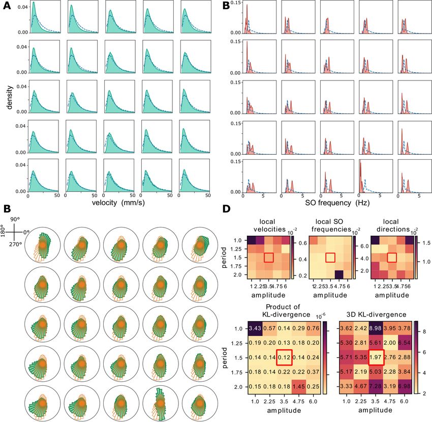
5Figure 2: Experimental data analysis. Outcomes of the developed analysis tools applied to the 8 sets of
experimental data (t1 − t8 ordered time sequences). A) local velocities distributions. B) local slow oscillation
(SO) frequencies distributions. C) local wave direction distributions. D) Kullback-Leibler divergence between
the observable distributions (local velocities, wave frequencies and directions) of the 8 datasets. The product
of these distributions is shown in the plot on the right.
6Figure 3: Dynamics comparison. A. Color-coded example of the time course of the firing rate activity for
each pixel, for the simulation and the data (top and bottom panels respectively). For visualization purposes
only 20s out of the 80s composing t2 and t3 are reported. B. Time course of the luminosity signal averaged
over all the pixels, for the simulation and the data (top and bottom panels respectively). Each pair of two
consecutive Up-states is marked with a red point when the delay between them is shorter then a certain
threshold, and marked with a blue point otherwise. The histograms of the inverse of those delays is reported
on the right. Long and short delays are represented in blue and red respectively. C. Comparison of the
power spectrum computed on the firing rate activity averaged over all the pixels. Data and simulations in
orange and green respectively. D. Phase diagram of the model. The green region is where oscillations occur.
Oscillation frequency is color-coded. The point (1,1) is the one inferred from the likelihood maximization.
The oscillatory external drive, oscillates around this point following the red and blue arrows. The blue arrow
brings the system to lower frequency and to a region of no oscillations. This explains the dark bands observed
in panel A and the long delays (blue) observed in B. The red arrow brings the system to a higher frequency
region, accounting for the short delays (red) in B.
7the variability of the slow oscillation (SO) frequency, could not be reproduced in the model with the inner
loop only. For this reason we decided to include an external neuro-modulation. This allowed to reproduce
the presence of longer down states in the model, when the neuro-modulation induces a reduction in the
excitability of the network (Fig.3A-top).
To better investigate this feature we considered the time course of the luminosity signal averaged over
all the pixels, for the simulation and the data (Fig.3B. top and bottom panels respectively). We evaluated
the time distance between two consecutive up-states and marked it with a red point when the delay between
them is shorter than a certain threshold, and marked with a blue point otherwise (longer Down states). The
histograms of the inverse of those delays, are reported on the right. Long and short delays are represented in
blue and red respectively. The histogram for experimental data displays a bimodal distribution; a bimodal
distribution is recovered in the simulation with the introduction of the neuro-modulation, that in addition
allows to obtain a remarkable similarity in the power spectrum computed on the firing rate activity averaged
over all the pixels (see Fig.3C, data and simulations in orange and green respectively).
A better understanding of this phenomenon can be obtained by considering the phase diagram of the
model reported in Fig.3D [17]. The green region represents the limit cycle region, where oscillations occur.
Oscillation frequency is color-coded. The point (1,1) identifies the values inferred from the likelihood maxi-
mization and belongs to the SO region (slow oscillations). The oscillatory external drive, oscillates around
this point along the red and blue arrows. The blue arrow brings the system to lower frequencies and to a
region of no oscillations, the LAS region (Low-rate asynchronous state), where a state with a low level of
activity is the fixed point. The High-rate activity state (HAS region), characterized by the fact that the
stable fixed point is a state with a high level of activity, is never accessed by our model. This explains the
dark bands observed in panel Fig.3A and the long delays (blue) observed in Fig.3B. The red arrow brings
the system to a higher frequency region, accounting for the short delays (red) in Fig.3B.
Two-step inference method
The Inner Loop
The first step of the inference method we propose can be seen as a one-way flow of information from data to
the model and consists in estimating parameters by likelihood maximization, see Fig4A.
We built a generative model as a network of interacting population of (AdEx) neurons. Each population
is modeled by a first order mean field equation [15, 17, 6, 4]. In other word all the neurons in the population
are described by their average firing rate. The neurons are affected by spike frequency adaptation, that is
accounted for by an additional equation for each population (see methods for details).
We remark that we considered current-based neurons, however the mean field model might be extended
to the conductance-based case [14, 8].
The single population aims at modeling the group of neurons recorded by a single pixel (after the under
sampling is performed, see Methods for details).
Single neuron parameters (membrane potential, threshold and so on) are reported in TABLE I in the
Methods section. The other parameters, the connectivity, the external currents and the adaptation are
inferred from the data. This is achieved by defining the likelihood L for the parameters {ξ} to describe a
specific observed dynamics {S} (see Methods section for details)
X (Si (t + dt) − Fi (t))2
L({S}|{ξ}) = − (1)
it
2c2
where Fi (t) is the transfer function of the population i and c is the variance of the Gaussian distribution
from which the activity is extracted (see Methods for details, Generative model section). We remark that in
this work we consider populations composed of excitatory/inhibitory neurons. To model this it is necessary
to use an effective transfer function describing the average activity of the excitatory neurons and accounting
for the effect of the inhibitory neurons (see Methods for details, Excitatory-Inhibitory module, the effective
transfer function section).
The optimal parameters are inferred from maximizing such a likelihood with respect to the parameters.
The optimizer we used is iRprop, a gradient based algorithm [23].
8Figure 4: Inner Loop. A. The first step of our inference method is a one-way flow of information from data
to the model and consists in estimating parameters by likelihood maximization. B,C,D,F,G,H. Spatial maps
of estimated parameters. The parameters are k0 , φ, e, λ, and a are the connectivity parameter, as defined
in Methods, Iext and b which are the local external input and the strength of the adaptation. E. Example
of 10 inferred elliptic connectivity kernels. They show the existence of strong eccentricity (e and a) and
prevalent orientations (φ) for the elliptic connectivity kernels, that facilitate the initiation and propagation
of wave-fronts along preferential axes, orthogonal to the major axis of the ellipses. I. The values of likelihood
and validation likelihood (respectively in in blue and orange) as a function of the number of iterations.
9The parameters are not assumed to be homogeneous in the space and each population is left free to have
different inferred parameters. The resulting parameters are reported in Fig.4B,C,D,F,G,H. Each panel
represents, color-coded, the spatial map of a different inferred parameter, describing its distribution over the
cortex of the mouse. Specifically, 1) the parameters that characterize at local level the inferred shape of
the elliptical exponential decaying connectivity kernels (see Methods, section Elliptic, exponentially decaying,
connectivity kernels) are: λ, k0 , φ, e, a; 2) b is the strength of the spike frequency adaptation (see section
Generative Model and Eq.4) 3) Iext is the local external input current. Panel E in Fig.4E presents, for a
few exemplary pixels, the total amount of connectivity incoming from the surrounding region, and shows the
existence of strong eccentricity (e and a) and prevalent orientations (φ) for the elliptic connectivity kernels,
that facilitate the initiation and propagation of wave-fonts along preferential axes, orthogonal to the major
axis of the ellipses.
In principle such parameters define the generative model which better reproduce the experimental data.
A major risk while maximizing the likelihood (see Fig.4 G, blue line) is the over-fitting, which we avoid by
considering the validation likelihood (see Fig.4 G - orange line), a likelihood evaluate on data expressing
the same kind of dynamics but not used for the inference. The likelihood increase associated to a validation
likelihood decrease is an alarm for over-fitting.
Inferred models at different times in the inner loop account for different anesthesia levels
To give an overview of the likelihood maximization results, parameters are inferred independently in all
the 8 chunks reported in Fig1B. In Fig.5(top) it is reported the Pearson correlation coefficient between
parameters inferred in the different chunks (External current, Adaptation and connectivity respectively). In
Fig.5(bottom) it is reported the median value (black), Q1, and Q3 (red) of the inferred parameters for the 8
chunks (External current, Adaptation and connectivity respectively).
Figure 5: Inference at different times in the inner loop. To give an overview of the likelihood maxi-
mization results, parameters are inferred independently in all the 8 chunks reported in Fig1.B. (top) Pearson
correlation coefficient between parameters inferred in the different chunks (External current, Adaptation and
connectivity respectively). (bottom) Average value of inferred parameters for the 8 chunks (External current,
Adaptation and connectivity respectively).
10The Outer Loop
The likelihood maximization constraints the following step in the dynamics as a function of the state of the
network at the previous step. Therefore the inferred parameters should give a good prediction of the activity
of the network at the following time step. It is indeed not trivial that the spontaneous activity performed by
the model reproduces the desired variety of dynamical properties observed in the data.
We run the spontaneous mean field simulation for the same duration of the original recording.
We found that parameters estimated in the first step provide a generative model capable to reproduce
oscillations and traveling wavefronts. However the activity produced by the model inferred from the inner
loop results to be much more regular if compared to the experimental one. Indeed, the down state duration
and the wavefront shape are almost always the same. Moreover some parameters cannot be optimized by
likelihood maximization. For this reason it is necessary to introduce the outer loop described in this section.
First, we analyze the spontaneous activity of the generative model and compare it to the data to optimize
parameters that cannot be optimized by likelihood differentiation (see Fig.6A). Then, we include in the
model an external oscillatory neuro-modulation (inspired by [18], but then we look for optimal amplitude
and period for such neuromodulation proxy. Such a neuro-modulation affects both the values of Iext and b
(more details in Methods section).
Figure 6: Outer Loop. A. The second step of the method consists in comparing simulations and data to op-
timize hyper-parameters (Amplitude and Period of the external drive). B,C,D. Kullback-Leibler divergence
between distributions (waves’ frequency, velocity, and directions respectively) in data (t2,t3) and simulations
(parameters inferred from t2,t3). The optimal point results to be period = 1.5s, amplitude = 3.5. E.
Kullback-Leibler divergence between distributions (waves’ frequency, velocity, and directions respectively) in
data (t2,t3) in the 3D space. F,G,H. Direct comparison of the distributions for the optimal point (waves’ fre-
quency, velocity, and directions respectively). I. Distribution in the 3D space of simulation output performed
with the set of parameters associated to the minimum value of the 3D-Kullback-Leibler divergence. Each
point is a pixel, and each color is a different wave. The coordinate of the points are local waves’ frequency,
velocity, and directions.
We performed a grid-search in the space (amplitude,period), and considered 3 different observables:
waves’ frequency, velocity, and direction. In Fig.6B,C,D it is reported the Kullback-Leibler divergence
between distributions (waves’ frequency, velocity, and directions respectively) in data (t2,t3) and simulations
(parameters inferred from t2,t3) for different values of (amplitude,period). The optimal point results to be
period = 1.2s, amplitude = 3.5.
In Fig.6E we report the Kullback-Leiber divergence between the 3-dimensional distributions in data and
11simulation (each point in the 3D space is associated to the local velocity, direction and frequency of the wave,
as shown in Fig.6I for the simulation performed with the optimal point parameters). Accordingly with the
results obtained for each observable individually, the optimal point (the one where the KL is minimum) also
results to be in period = 1.2s, amplitude = 3.5. In Fig.6F,G,H we show the direct comparison between
the distributions of waves’ frequency, velocity, and directions respectively for the the optimal point in the
parameters space.
Methods
Mouse wide-field calcium imaging
In vivo calcium imaging datasets have been provided by LENS (European Laboratory for Non-Linear Spec-
troscopy1 ). All the procedures were performed in accordance with the rules of the Italian Minister of Health
(Protocol Number 183/2016-PR). Mice were housed in clear plastic enriched cages under a 12 h light/dark
cycle and were given ad libitum access to water and food. To monitor neuronal activity the transgenic mouse
line C57BL/6J-Tg(Thy1GCaMP6f)GP5.17Dkim/J (referred to as GCaMP6f mice2 ) from Jackson Laborato-
ries (Bar Harbor, Maine USA) was used. This mouse model selectively express the ultra-sensitive calcium
indicator (GCaMP6f) in excitatory neurons.
Surgery procedures and imaging: 6 months old male mice were anaesthetized with a mix of Ketamine
(100 mg/kg) and Xylazine (10 mg/kg). To obtain optical access to the cerebral mantle below the intact
skull, the skin and the periosteoum over the skull were removed following application of the local anesthetic
lidocaine (20 mg/mL). Imaging sessions were performed right after the surgical procedure. Wide-field
fluorescence imaging of the right hemisphere were performed with a 505 nm LED light (M505L3 Thorlabs,
New Jersey, United States) deflected by a dichroic mirror (DC FF 495-DI02 Semrock, Rochester, New York
USA) on the objective (2.5x EC Plan Neofluar, NA 0.085, Carl Zeiss Microscopy, Oberkochen, Germany).The
fluorescence signal was selected by a band-pass filter (525/50 Semrock, Rochester, New York USA) and
collected on the sensor of a high-speed complementary metal-oxide semiconductor (CMOS) camera (Orca
Flash 4.0 Hamamatsu Photonics, NJ, USA). A 3D motorized platform (M-229 for the xy plane, M-126 for
the z-axis movement; Physik Instrumente, Karlsruhe, Germany) allowed the correct subject displacement in
the optical setup.
Experimental Data and Deconvolution
We assume that the optical signal Xi (t) acquired from each pixel i is proportional to the local average
excitatory (somatic and dendritic) activity (see Fig1-top right). The main issue is the slow response of the
calcium indicator (GCaMP-6f). We estimate the shape of such a response function from the single spike
response [10] as a log-normal function
t
2 !
−µ
t dt 1 ln dt
LN ; µ, σ = √ exp − , (2)
dt t 2πσ 2σ 2
where dt = 40ms, and µ = 2.2 and σ = 0.91 as estimated in [9]. After approximating as linear the
response of the calcium indicator (which is known to be not exactly true) we apply the deconvolution to
obtain an extimation of the actual firing rate time course Si (t). The deconvolution is simply achieved by
dividing the signal by the lognormal in the fourier space.
X̂i (k)
ŜI (k) = Θ(k − k0 ) (3)
ˆ (k)
LN
Where X̂i (k) = f f t(Xi (t)) and LN ˆ (k) = f f t(LN ˆ (t)) (f f t(·) is the fast fourier transform). Finally
the deconvolved signal is Ŝi (t) = if f t(Si (k)) (if f t(·) is the inverse fast fourier transform). The function
Θ(k − k0 ) is the heaviside functions and is used to apply a low pass filter with a cutoff frequency k0 = 6.25Hz.
1 LENS Home Page, http://www.lens.unifi.it/index.php
2 For more details, see The Jackson Laboratory, Thy1-GCaMP6f, https://www.jax.org/strain/025393.
12Generative Model
We assume a system composed of Npop (approximately 1400) interacting populations of neurons. Population
j at time t has a level of activity (firing rate) defined by the variable Sj (t) = {0, 1, 2....}. Each population j
is associated to a pixel j of the experimental optical acquisition.
Each population j is composed of Nj neurons, Jij and Cij are the average synaptic weight and the average
degree of connectivity between the populations i and j. We define the parameters kij = Nj Jij Cij , that are
the relevant ones in the inference procedure.
We also consider that each population receives an input from a virtual external populations composed of
Njext neurons, each of which injecting a current Jjext in the population with a frequency νjext . Similarly to
what was done above, we define the parameter Ijext = νjext Njext Jjext .
In a common formalism site i at time t is influenced by the activity of other sites through couplings kik
[3], in term of a local input current defined as
X
µi (t) = kik Sk (t) + Iiext − bi Wi (t) (4)
k
The term bi Wi (t) accounts for a feature that plays an essential role in modeling the emergence of cortical
slow oscillations is the spike frequency state-dependent adaptation, the progressive tendency of neurons to
fatigue and reduce their firing rates even in the presence of constant excitatory input currents. Spike frequency
adaptation is know to be much more pronounced in deep-sleep and anaesthesia than during wakefulness. From
a physiological stand-point, this is associated to the calcium concentration in neurons and can be modeled
introducing a negative (hyper-polarizing) current on population i, the bi Wi (t) term in eq.4. W (t) is a fatigue
variable: it increases when neuron i emits a spike and is gradually restored to its rest value when no spikes
are emitted, and its dynamics can be written as
Wi (t + dt) = (1 − αw )Wi (t) + αw Sk (t + dt) (5)
where αw = 1 − exp(−dt/τw ), and τw is the characteristic time scale of SFA.
It is also customary to introduce (adaptation couplings) bi that determine how much the fatigue influences
the dynamics: this factor changes depending on neuro-modulation and explains the emergence of specific
dynamic regimes associated to different brain states. Specifically, higher value of b (together with higher
values of recurrent connectivity) are used in models to the induction of Slow Oscillations, as illustrated by
Fig.4.D.
It is also possible to write down the dynamics for the activity variables by assuming that the probability
at time t + dt to have a certain level of activity Si (t + dt) in the population i is drawn from a gaussian
distribution:
(Si (t + dt) − Fi (t)))2
1
p(Si (t + dt)|S(t)) = p(Si (t + dt)|Fi (t)) = √ exp − . (6)
2πc2 2 c2
For simplicity we assumed c to be constant in time, and the same for all the populations. The temporal
dynamics of such a variable might be accounted by considering a second order mean field theory [15, 11].
The average activity of the population ν(t + dt) at time t + dt is computed as a function of its input by
using a leaky integrate and fire response function
hSi (t + dt)i = F [µi (t), σi2 (t)] := Fi (t) (7)
where F (µi (t), σi2 (t))
is the transfer function that for an AdEx neuron, under stationary conditions, can
be analytically expressed as the flux of realizations (i.e., the probability current) crossing the threshold
Vspike = θ + 5∆V [43, 8]:
Z θ+5∆V Z θ+5∆V
2 1 −τ 1
Ru
[f (v)+µτm ]dv
F (µ) = lim F (µ, σ ) = lim dV due m σ2 V
. (8)
σ→0 σ→0 σ2 −∞ max(V,Vr )
13Table 1: Neuronal parameters defining the two populations RS-FS model.
θ (mV) τm (ms) C (nF) El (mV) ∆V (mV) τi (ms) Ei (mV) Qi (nS) b (nA) τW (s)
exc -50 20 0.2 -65 2.0 5 0 1 0.005 0.5
inh -50 20 0.2 -65 0.5 5 -80 5 0 0.5
v(t)−θ
where f (v) = −(v(t) − El ) + ∆V e( ∆V ) , τm the membrane time constant, C the membrane capacitance,
El the reversal potential, θ the threshold, ∆V the exponential slope parameter. The parameter values are
reported in the table below. Here we considered the limit for small and constant σ, since we assume small
fluctuations, and however that the fluctuations have a small effect on the population dynamics. We will
verify such assumption a posteriori. It is actually straightforward to work out the same theory not making
assumption on the size of σ, the only drawback is an increased computational power required to evaluate a
2d function during the inference (and simulation) procedure.
The Inner Loop: likelihood maximization
It is possible to write the log-likelihood of one specific history {Si (t)} of the dynamics of the model, given
the parameters {ξk }, as follows:
X (Si (t + dt) − Fi (t))2
L({S}|{ξ}) = − (9)
it
2c2
The optimal parameters, given an history of the system {S(t)}, can be obtained by maximizing the
likelihood L({ξk }|{S}). When using a gradient-based optimizer (we indeed use iR-prop) it is necessary to we
computed the derivatives that can be written as
∂L({S}|{ξ}) X (Si (t + dt) − Fi (t)) ∂Fi (t) ∂µ
=− (10)
∂ξk it
c2 ∂µ ∂ξk
where ∂F∂µ
i (t) ∂µ
are computed numerically while ∂λ k
ca be easily evaluated analytically.
For the optimization procedure 2 data chunks of 40s each are considered (t2-t3). For each chunk param-
eters are optimized on the first 32s while the remaining 8s are used for validation. The likelihood on such
a dataset is evaluated with the inferred parameters, this is referred to as validation likelihood. It helps to
prevent the risk of overfitting.
All the parameters are optimized on the all dataset, with the only exception of the b parameter. Indeed
we inferred a global multiplicative factor independently for t2 and t3. We find that the adaptation is stronger
in t3 (approximately by a factor 1.2).
Excitatory - Inhibitory module, the effective transfer function
In this paper, the single population (pixel) is assumed to be composed of two sub-populations of excitatory
and inhibitory neurons the mean of the input currents reads as:
e P ee e P ei i e
µi (t) = k kik Sk (t) + k kik Sk (t) + Iext − bi Wi (t)
(11)
i P ie e P ii i i
µi (t) = k kik Sk (t) + k kik Sk (t) + Iext
It is not always possible to distinguish the excitatory S e from the inhibitory firing rates S i in experimental
recordings. Indeed, in electrical recordings the signal is a composition of the two activities. However, in our
case we can make the assumption that the recorded activity, after the deconvolution, is a good proxy of the
excitatory activity S e . This is possible thanks to the fluorescent indicator we considered in this work which
14targets specifically excitatory neurons. In this way it is possible to constrain the excitatory activity and to
consider S i as hidden variable.
In this case the transfer function depend both on the excitatory and the inihibitory activities Fe (S e , S i ).
However S i is not observable in and it is necessary to estimate an effective transfer function for the excitatory
population of neurons by making an adiabatic approximation on the inhibitory one [26]. We define the
effective transfer function as
F (S e ) = Feef f (S e ) = Fe (S e , S i (S e )) (12)
The inhibitory activity S i is assumed to have a faster timescale (which is biologically true, inhibitory
neurons are indeed called fast spiking neurons). As a consequence S i (S e ) can be evaluated as its stationary
value given a fixed S e value.
The likelihood than contains this new effective transfer function, is a function of k ee and k ei , which
are the weights to be optimized. The dependence on k ie , k ii disappears, they have to be suitably chosen
(k ie = k ii = −25 in our case) and cannot be optimized with this approach.
Elliptic, exponentially decaying, connectivity kernels
To have a large number of parameters, especially in the case of small datasets, can create convergence
problems and increase the risk of over-fitting. However, experimental constraints and priors can be used
to reduce the number of parameters to be inferred. In our case we decided to exploit the information that
the lateral connectivity decays with the distance, in first approximation according to a simple exponential
reduction law [38], with long-range inter-areal connection suppressed during the expression of slow-waves
[31]. Furthermore, we supposed that a deformation from a circular simmetry to a more elliptical shape of the
probability of connection could facilitate the creation of preferential directions of propagation. Therefore,
we included this in the model as an exponential decay on the spatial scale λ. In this case the average input
current to the population i can be written as
X j dij
µi (t) = kik Sk (t) + Iext − bi Wi (t), kij = k0 exp − (13)
λj
k
where dik is the distance between the population i and k.
dik = ρik (1 + ek cos(2θik + 2φk )) (1 + ak cos(θik + φk )) (14)
All the parameters can be inferred by differentiating such parametrization of the connectivity kernel. As
an example the derivative respect to the spatial scale λk to feed into eq.(10) would be
∂µi (t) dik
= kik Sk (t) 2 (15)
∂λk λk
Slow Waves and Propagation analysis
To analyze and compare the simulation outputs with experimental data we implemented and applied the
same analysis tools to both data sets. Specifically, we improved the pipeline described by some of us in [9] to
make it more versatile. First, experimental data are arranged to make them suitable for both the application
of the Slow wave propagation analysis and the inference method. Thus, data are loaded and converted into a
standardized format, region of interest is selected by masking channels of low signal intensity. Fluctuations
are further reduced applying a spatial downsampling: pixels are assembled in 2x2 blocks though the function
scipy.signal.decimate [46] curating the aliasing effect through the application of an ideal Hamming Filter.
Now data are ready to be both analyzed or given as input to the inference method.
Both experimental data and simulation output can then be given as input to these analysis tools. The
procedure we followed is articulated into four main blocks.
15• Processing: The constant background signal is estimated for each pixel as the mean of the signal
computed on the whole image set; it is then subtracted from images, pixel by pixel. The signal is then
filtered at with a 4th order batterworth filter at 6Hz. The resulting signal is then normalized by its
maximum.
• Trigger Detection: transition times from down to Up states are then detected. These are identified
from the local signal minima. Specifically, the collection of transition times for each channel is obtained
as the vertex of the parabolic fit of the minima.
• Wave Detection: the detection method used in [9] and described in [12]. This consists in splitting the
set of transition times into separate waves according to a Unicity Principle (i.e. each pixel can be
involved in each wave only once) and a Globality principle (i.e. each Wave needs to involve at least
75% of the total pixel number).
• Wave Characterization: to characterized the provided data we measure the local wave velocity, local
wave direction and local SO frequency.
Specifically, we compute the local wave velocity as
1 1
v(x, y) = = r (16)
|∇T (x, t)| ∂T (x,y)
2 2
∂x + ∂T∂y
(x,y)
where T (x, y) is the the passage time function of each wave. Having only access to this function only in the
pixel discrete domain, the partial derivatives have been calculated as finite differences as follows:
∂T (x, y) T (x + d, y) − T (x − d, y)
'
∂x 2d
∂T (x, y) ' T (x, y + d) − T (x, y − d) .
∂y 2d
where d is the distance between pixels. Concerning local directions, for each wave transition we compute a
weighted average of wave local velocities components through a Gaussian filter w(µ,σ) centered in the pixel
involved in the transition and with σ = 2. The local direction associated to the transition is
!
hv y i w
θ(x, y) = tan−1
(y,σ)
(17)
hvx iw(x,σ)
Finally, the SO local frequency is computed as the inverse time lag of the transition on the same pixel by
two consecutive waves. Defining T (w) (x, y) as the transition time of wave w on pixel (x, y), the SO frequency
can thus be computed as:
1
SOF req (1,2) (x, y) = (2) (18)
T (x, y) − T (1) (x, y)
Neuro-modulation
The periodic neuro-modulation we included in our network was modeled as a periodic oscillations of the
parameters b and I ext described by the following equations:
2πt
ext ext,0
Ii (t) = Ii 1 + A cos
T
(19)
A 2πt
bi (t) = b0i 1 +
cos
6 T
where we defined Iiext,0 and b0i as the set of parameters inferred in the inner loop over the whole dataset
composed of the t2 and t3 recordings, while A and T are the amplitude and the oscillation period optimized
in the outer loop.
16Actually, the adaptation strengths in t2 and t3 are inferred independently. We account for this including a
very slow neuro-modulation, whose timescale is 80s. In the simulation we slowly varied the bi by multiplying
f in
it by a factor which changes from an initial (bin f act = 0.93) to a final value (bf act = 1.2).
The final expression for bi (t) is the following:
0 tf in − t in t − tf i f in A 2πt
bi = bi (t) b + b 1+ cos (20)
tf in − tin f act tf in − tin f act 6 T
where tin = 0s and tf in = 80s.
The Outer Loop: grid search and data-simulation comparison
There can be different ways to define the outer loop. One way might be an iterative algorithm where at each
step the simulations and data are compared and parameters are updated with some criterion.
Here we use a simpler strategy, we implement a grid search of the parameters to be optimized to find
the best match. The parameters we considered are A and T, namely the amplitude and the period of the
neuro-modulation. We run a 5x5 grid with parameter A linearly ranging from 1 to 6 and parameter T linearly
ranging from 1s to 2s.
We analyzed each simulation by evaluating the distributions of waves frequencies, speeds and directions
(see Fig.7). These distributions are directly compared with the respective distribution evaluated in the ex-
perimental recording. The quality of the match is evaluated though the Kullback-Leibler divergence between
the experimental and the simulated distributions.
Discussion
In recent years, the field of statistical inference applied to neuronal dynamics has mainly focused on the
reliably estimate of an effective synaptic structure of a network of neurons [36, 44, 30]. To our knowledge,
the investigation of the dynamics of the inferred models has been largely neglected. However, we are not the
first to address the issue. In [34] the authors demonstrated, on an in-vitro population of ON and OFF parasol
ganglion cells, the ability of a Generalized Linear Model (GLM) to accurately reproduce the dynamics of the
network [32]; studied the response properties of lateral intraparietal area neurons at the single trial, single
cell level; the capability of GLM to capture a broad range of single neuron response behaviors was analyzed
in [47]. However, in these works, the focus was on the response of neurons to stimuli of different spatio-
temporal complexity. Moreover recurrent connections, where accounted for, where not a decisive correction
to the network dynamics. A very few published study to date has focused on the autonomous dynamics of
networks inferred from neuronal data. Most of them focused on the resting state recorded through fMRI
and on the reproduction of its functional connectivity[2]. In [3] the temporal and spatial features of bursts
propagation have accurately reproduced, but on a simpler biological system, a culture of cortical neurons
recorded with a 60 electrodes array. Here we aim at reproducing the dynamics of the whole hemisphere of
the mouse with approximately 1400 recording sites.
One of the major risk when inferring a model is the failure of the generative to reproduce a dynamics
comparable to the data. The reason for this is that when inferring the models some of the observables
are not easy to constrain. A common example is offered by the Ising model. When inferring its coupling
and external fields, only magnetizations and correlations between different spins are constrained [37], but
it is not possible to constrain the power spectrum displayed by the model and other temporal features.
When this experiment is done on the Ising model itself, this is not a problem. When the dataset is large
enough the correct parameters are inferred and also the temporal features are correctly reproduced. However
if the original model contains some hidden variable (unobserved neurons, higher-order connectivity, other
dynamical variables), the dynamics generated by the inferred model might not be descriptive of the original
dynamics. This lead us to introduce the two steps method, in order to adjust parameters beyond likelihood
maximization.
Another obvious but persisting problem in the application of inference models to neuroscience has been
how to assess the meaning and value of the inferred parameters. In the literature, a cautionary remark is
17Figure 7: Grid search over Amplitude and Period of the external stimulus on simulated data.
A) Grid Search outcomes over local wave velocities distributions. Blue dotted lines depict the experimental
distribution. The amplitude values increases with the column (specifically, from 1.0 to 6.0) whereas the
period value increases with the row (specifically, from 1.0 to 1.5).The local velocities are computed according
to equation 16. B Grid Search outcomes concerning the local SO frequencies distributions. Blue dotted lines
depict the experimental distribution. The amplitude values increases with the column (specifically, from 1.0
to 6.0) whereas the period value increases with the row (specifically, from 1.0 to 1.5).The local SO oscillation
frequencies are computed as the inverse of the lag between transitions times of two consecutive waves in
the same channel. C. Grid Search outcomes concerning the local wave directions. Orange solid lines depict
the experimental distribution. The amplitude value increases with the column (specifically, from 1.0 to 6.0)
whereas the period value increases with the row (specifically, from 1.0 to 1.5).The local wave directions are
computed as according to equation 17. D. Kullback-Leibler divergence between distributions (local waves’
frequency, velocity, directions and their product) in data and simulations (parameters inferred from t2,t3).
The optimal point results to be period = 1.25s, amplitude = 4.75.
18usually included, recognizing that the inferred couplings are to be meant as ‘effective’, leaving of course open
the problem of what exactly this means.
One way to infer meaningful parameters is to introduce good priors. In this work we assume that under
anesthesia inter-areal connectivity largely suppressed in favor of lateral connectivity, as demonstrated e.g. in
[31]. Also, the probability of lateral connectivity in the cortex is experimentally known [38] to decay with
the distance according to an exponential decay, with the decay parameter in the range of a few hundreds of
µm. For this reason, we introduced exponentially decaying elliptical connectivity kernels in our model. The
hypothesis of elliptical and non circular kernels was related to the knowledge that preferential directions for
the propagation of cortical slow-waves are manifest in the data [7], and the alignment of the major axes of
elliptical sources support the creation of such preferential directions. We remark that inferring connections at
this mesoscopic scale allows obtaining information that is complementary to the one contained in inter-areal
connectivity atlas, where connectivity is considered on a larger spatial scale and its is carried by white-matter,
and not by lateral connectivity. A key feature of neural networks is Degeneracy, the ability of systems that
are structurally different to perform the same function [42]. Also, generic atlases of Structural Connectivity
(SC) and Functional Connectivity (FC) contain information averaged among different individuals. Similar
functions and dynamics can be sustained in each individual by specific SC and FCs. [27] [25]. Our approach
allows inferring (in-vivo) an individual connectivity. This is a contribution to the the construction of brain-
specific models from in-vivo data, descriptive of the dynamical features observed in one specific individual.
One of the values added by the modeling technique here described is that its dynamics relies on a mean
field theory which describes populations of interconnected spiking neurons. This is particularly useful to set
up a richer and more realistic dynamics in large scale spiking simulation of SWA and AW activity [33] that in
absence of such details inferred parameters behave according to quite stereotyped spatio-temporal features.
In perspective, we plan to integrate plastic cortical modules capable of incremental learning and sleep
and demonstrating the mechanism producing the beneficial cognitive effects of sleep [6, 19] on small scale
networks with the methodology here described. This combination will support the construction of plastic
models demonstrating the cognitive effects of cortical slow waves at the scale of larger portions of the thalamo-
cortical system.
Finally, we plan to go beyond spontaneous activity, aiming at modeling the dynamics of the network when
it receives input signals, ranging from simple perturbations to sensory stimuli. The methodology to achieve
this would be very similar to what presented in [29, 13].
Acknowledgments
This work has been supported by the European Union Horizon 2020 Research and Innovation program under
the FET Flagship Human Brain Project (grant agreement SGA3 n. 945539 and grant agreement SGA2 n.
785907) and by the INFN APE Parallel/Distributed Computing laboratory.
References
[1] Walther Akemann et al. “Imaging neural circuit dynamics with a voltage-sensitive fluorescent protein”.
In: Journal of neurophysiology 108.8 (2012), pp. 2323–2337.
[2] Marco Aqil et al. “Graph neural fields: A framework for spatiotemporal dynamical models on the human
connectome”. In: PLOS Computational Biology 17.1 (Jan. 2021), pp. 1–29. doi: 10.1371/journal.
pcbi.1008310. url: https://doi.org/10.1371/journal.pcbi.1008310.
[3] Cristiano Capone, Guido Gigante, and Paolo Del Giudice. “Spontaneous activity emerging from an
inferred network model captures complex spatio-temporal dynamics of spike data”. In: Scientific reports
8.1 (2018), p. 17056.
[4] Cristiano Capone and Maurizio Mattia. “Speed hysteresis and noise shaping of traveling fronts in neural
fields: role of local circuitry and nonlocal connectivity”. In: Scientific reports 7.1 (2017), pp. 1–10.
[5] Cristiano Capone et al. “Inferring synaptic structure in presence of neural interaction time scales”. In:
PloS one 10.3 (2015), e0118412.
19You can also read