DDSP: DIFFERENTIABLE DIGITAL SIGNAL PROCESSING
←
→
Page content transcription
If your browser does not render page correctly, please read the page content below
Published as a conference paper at ICLR 2020

                                         DDSP:
                                         D IFFERENTIABLE D IGITAL S IGNAL P ROCESSING
                                          Jesse Engel, Lamtharn Hantrakul, Chenjie Gu, & Adam Roberts
                                          Google Research, Brain Team
                                          Mountain View, CA 94043, USA
                                          {jesseengel,hanoih,gcj,adarob}@google.com

                                                                                      A BSTRACT
arXiv:2001.04643v1 [cs.LG] 14 Jan 2020

                                                  Most generative models of audio directly generate samples in one of two domains:
                                                  time or frequency. While sufficient to express any signal, these representations are
                                                  inefficient, as they do not utilize existing knowledge of how sound is generated
                                                  and perceived. A third approach (vocoders/synthesizers) successfully incorpo-
                                                  rates strong domain knowledge of signal processing and perception, but has been
                                                  less actively researched due to limited expressivity and difficulty integrating with
                                                  modern auto-differentiation-based machine learning methods. In this paper, we
                                                  introduce the Differentiable Digital Signal Processing (DDSP) library, which en-
                                                  ables direct integration of classic signal processing elements with deep learning
                                                  methods. Focusing on audio synthesis, we achieve high-fidelity generation with-
                                                  out the need for large autoregressive models or adversarial losses, demonstrating
                                                  that DDSP enables utilizing strong inductive biases without losing the expressive
                                                  power of neural networks. Further, we show that combining interpretable modules
                                                  permits manipulation of each separate model component, with applications such
                                                  as independent control of pitch and loudness, realistic extrapolation to pitches not
                                                  seen during training, blind dereverberation of room acoustics, transfer of extracted
                                                  room acoustics to new environments, and transformation of timbre between dis-
                                                  parate sources. In short, DDSP enables an interpretable and modular approach to
                                                  generative modeling, without sacrificing the benefits of deep learning. The library
                                                  is publicly available1 and we welcome further contributions from the community
                                                  and domain experts.

                                         1    I NTRODUCTION
                                         Neural networks are universal function approximators in the asymptotic limit (Hornik et al., 1989),
                                         but their practical success is largely due to the use of strong structural priors such as convolution (Le-
                                         Cun et al., 1989), recurrence (Sutskever et al., 2014; Williams & Zipser, 1990; Werbos, 1990), and
                                         self-attention (Vaswani et al., 2017). These architectural constraints promote generalization and
                                         data efficiency to the extent that they align with the data domain. From this perspective, end-to-end
                                         learning relies on structural priors to scale, but the practitioner’s toolbox is limited to functions that
                                         can be expressed differentiably. Here, we increase the size of that toolbox by introducing the Differ-
                                         entiable Digital Signal Processing (DDSP) library, which integrates interpretable signal processing
                                         elements into modern automatic differentiation software (TensorFlow). While this approach has
                                         broad applicability, we highlight its potential in this paper through exploring the example of audio
                                         synthesis.
                                         Objects have a natural tendency to periodically vibrate. Small shape displacements are usually
                                         restored with elastic forces that conserve energy (similar to a canonical mass on a spring), leading
                                         to harmonic oscillation between kinetic and potential energy (Smith, 2010). Accordingly, human
                                         hearing has evolved to be highly sensitive to phase-coherent oscillation, decomposing audio into
                                         spectrotemporal responses through the resonant properties of the basilar membrane and tonotopic
                                            1
                                              Online Resources:
                                         Code: https://github.com/magenta/ddsp
                                         Audio Examples: https://goo.gl/magenta/ddsp-examples
                                         Colab Demo: https://goo.gl/magenta/ddsp-demo

                                                                                             1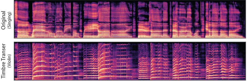
Published as a conference paper at ICLR 2020

mappings into the auditory cortex (Moerel et al., 2012; Chi et al., 2005; Theunissen & Elie, 2014).
However, neural synthesis models often do not exploit this periodic structure for generation and
perception.

1.1   C HALLENGES OF N EURAL AUDIO S YNTHESIS

As shown in Figure 1, most neural synthesis models generate waveforms directly in the time domain,
or from their corresponding Fourier coefficients in the frequency domain. While these representa-
tions are general and can represent any waveform, they are not free from bias. This is because they
often apply a prior over generating audio with aligned wave packets rather than oscillations. For ex-
ample, strided convolution models–such as SING (Defossez et al., 2018), MCNN (Arik et al., 2019),
and WaveGAN (Donahue et al., 2019)–generate waveforms directly with overlapping frames. Since
audio oscillates at many frequencies, all with different periods from the fixed frame hop size, the
model must precisely align waveforms between different frames and learn filters to cover all possible
phase variations. This challenge is visualized on the left of Figure 1.
Fourier-based models–such as Tacotron (Wang et al., 2017) and GANSynth (Engel et al., 2019)–
also suffer from the phase-alignment problem, as the Short-time Fourier Transform (STFT) is a
representation over windowed wave packets. Additionally, they must contend with spectral leakage,
where sinusoids at multiple neighboring frequencies and phases must be combined to represent a
single sinusoid when Fourier basis frequencies do not perfectly match the audio. This effect can be
seen in the middle diagram of Figure 1.
Autoregressive waveform models–such as WaveNet (Oord et al., 2016), SampleRNN (Mehri et al.,
2016), and WaveRNN (Kalchbrenner et al., 2018)–avoid these issues by generating the waveform
a single sample at a time. They are not constrained by the bias over generating wave packets and
can express arbitrary waveforms. However, they require larger and more data-hungry networks, as
they do not take advantage of a bias over oscillation (size comparisons can be found in Table B.6).
Furthermore, the use of teacher-forcing during training leads to exposure bias during generation,
where errors with feedback can compound. It also makes them incompatible with perceptual losses
such as spectral features (Defossez et al., 2018), pretrained models (Dosovitskiy & Brox, 2016), and
discriminators (Engel et al., 2019). This adds further inefficiency to these models, as a waveform’s
shape does not perfectly correspond to perception. For example, the three waveforms on the right of
Figure 1 sound identical (a relative phase offset of the harmonics) but would present different losses
to an autoregressive model.

      Figure 1: Challenges of neural audio synthesis. Full description provided in Section 1.1.
1.2   O SCILLATOR M ODELS

Rather than predicting waveforms or Fourier coefficients, a third model class directly generates
audio with oscillators. Known as vocoders or synthesizers, these models are physically and percep-
tually motivated and have a long history of research and applications (Beauchamp, 2007; Morise
et al., 2016). These “analysis/synthesis” models use expert knowledge and hand-tuned heuristics to
extract synthesis parameters (analysis) that are interpretable (loudness and frequencies) and can be
used by the generative algorithm (synthesis).
Neural networks have been used previously to some success in modeling pre-extracted synthesis
parameters (Blaauw & Bonada, 2017; Chandna et al., 2019), but these models fall short of end-
to-end learning. The analysis parameters must still be tuned by hand and gradients cannot flow
through the synthesis procedure. As a result, small errors in parameters can lead to large errors in

                                                  2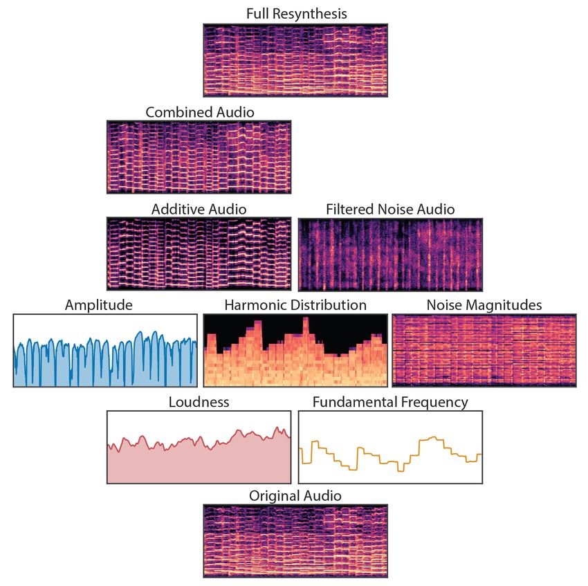
Published as a conference paper at ICLR 2020

the audio that cannot propagate back to the network. Crucially, the realism of vocoders is limited by
the expressivity of a given analysis/synthesis pair.

1.3      C ONTRIBUTIONS

In this paper, we overcome the limitations outlined above by using the DDSP library to implement
fully differentiable synthesizers and audio effects. DDSP models combine the strengths of the above
approaches, benefiting from the inductive bias of using oscillators, while retaining the expressive
power of neural networks and end-to-end training.
We demonstrate that models employing DDSP components are capable of generating high-fidelity
audio without autoregressive or adversarial losses. Further, we show the interpretability and modu-
larity of these models enable:

         •   Independent control over pitch and loudness during synthesis.
         •   Realistic extrapolation to pitches not seen during training.
         •   Blind dereverberation of audio through seperate modelling of room acoustics.
         •   Transfer of extracted room acoustics to new environments.
         •   Timbre transfer between disparate sources, converting a singing voice into a violin.
         •   Smaller network sizes than comparable neural synthesizers.

Audio samples for all examples and figures are provided in the online supplement2 . We highly
encourage readers to listen to the samples as part of reading the paper.

2       R ELATED W ORK

Vocoders. Vocoders come in several varieties. Source-filter/subtractive models are inspired by
the human vocal tract and dynamically filter a harmonically rich source signal (Flanagan, 2013),
while sinusoidal/additive models generate sound as the combination of a set of time-varying sine
waves (McAulay & Quatieri, 1986; Serra & Smith, 1990). Additive models are strictly more expres-
sive than subtractive models but have more parameters as each sinusoid has its own time-varying
loudness and frequency. This work builds a differentiable synthesizer off the Harmonic plus Noise
model (Serra & Smith, 1990; Beauchamp, 2007): an additive synthesizer combines sinusoids in
harmonic (integer) ratios of a fundamental frequency alongside a time-varying filtered noise signal.
Synthesizers. A separate thread of research has tried to estimate parameters for commercial syn-
thesizers using gradient-free methods (Huang et al., 2014; Hoffman & Cook, 2006). Synthesizer
outputs modeled with a variational autoencoder were recently used as a “world model” (Ha &
Schmidhuber, 2018) to pass approximate gradients to a controller during learning (Esling et al.,
2019). DDSP differs from black-box approaches to modeling existing synthesizers; it is a toolkit of
differentiable DSP components for end-to-end learning.
Neural Source Filter (NSF). Perhaps closest to this work, promising speech synthesis results were
recently achieved using a differentiable waveshaping synthesizer (Wang et al., 2019). The NSF can
be seen as a specific DDSP model, that uses convolutional waveshaping of a sinusoidal oscillator
to create harmonic content, rather than additive synthesis explored in this work. Both works also
generate audio in the time domain and impose multi-scale spectrograms losses in the frequency
domain. A key contribution of this work is to highlight how these models are part of a common
family of techniques and to release a modular library that makes them accessible by leveraging
automatic differentiation to easily mix and match components at a high level.

3       DDSP C OMPONENTS

Many DSP operations can be expressed as functions in modern automatic differentiation software.
We express core components as feedforward functions, allowing efficient implementation on parallel
    2
        https://goo.gl/magenta/ddsp

                                                     3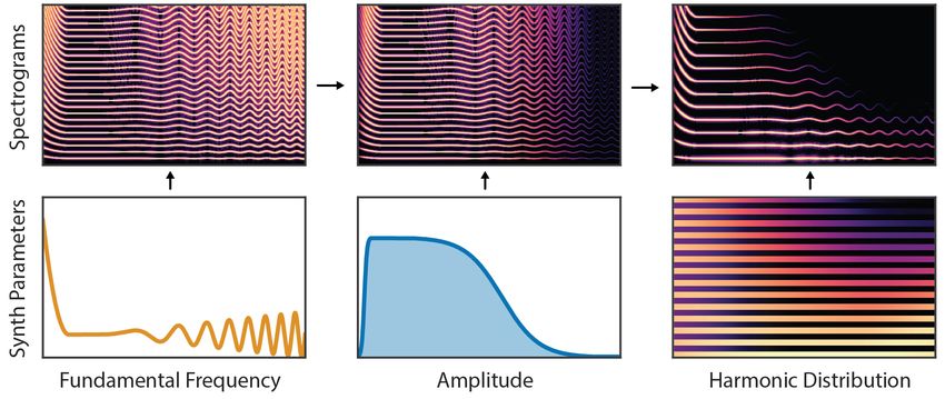
Published as a conference paper at ICLR 2020

hardware such as GPUs and TPUs, and generation of samples during training. These components
include oscillators, envelopes, and filters (linear-time-varying finite-impulse-response, LTV-FIR). 3

3.1   S PECTRAL M ODELING S YNTHESIS

Here, as an example DDSP model, we implement a differentiable version of Spectral Modeling
Synthesis (SMS) Serra & Smith (1990). This model generates sound by combining an additive
synthesizer (adding together many sinusoids) with a subtractive synthesizer (filtering white noise).
We choose SMS because, despite being parametric, it is a highly expressive model of sound, and has
found widespread adoption in tasks as diverse as spectral morphing, time stretching, pitch shifting,
source separation, transcription, and even as a general purpose audio codec in MPEG-4 (Tellman
et al., 1995; Klapuri et al., 2000; Purnhagen & Meine, 2000).
As we only consider monophonic sources in these experiments, we use the Harmonic plus
Noise model, that further constrains sinusoids to be integer multiples of a fundamental fre-
quency (Beauchamp, 2007). One of the reasons that SMS is more expressive than many other
parametric models because it has so many more parameters. For example, in the 4 seconds of
16kHz audio in the datasets considered here, the synthesizer coefficients actually have ∼2.5 times
more dimensions than the audio waveform itself ((1 amplitude + 100 harmonics + 65 noise band
magnitudes) * 1000 timesteps = 165,000 dimensions, vs. 64,000 audio samples). This makes them
amenable to control by a neural network, as it would be difficult to realistically specify all these
parameters by hand.

3.2   H ARMONIC O SCILLATOR / A DDITIVE S YNTHESIZER

At the heart of the synthesis techniques explored in this paper is the sinusoidal oscillator. A bank of
oscillators that outputs a signal x(n) over discrete time steps, n, can be expressed as:
                                             K
                                             X
                                    x(n) =         Ak (n) sin(φk (n)),                                 (1)
                                             k=1

where Ak (n) is the time-varying amplitude of the k-th sinusoidal component and φk (n) is its in-
stantaneous phase. The phase φk (n) is obtained by integrating the instantaneous frequency fk (n):
                                                   n
                                                   X
                                    φk (n) = 2π          fk (m) + φ0,k ,                               (2)
                                                   m=0

where φ0,k is the initial phase that can be randomized, fixed, or learned.
For a harmonic oscillator, all the sinusoidal frequencies are harmonic (integer) multiples of a funda-
mental frequency, f0 (n), i.e., fk (n) = kf0 (n), Thus the output of the harmonic oscillator is entirely
parameterized by the time-varying fundamental frequency f0 (n) and harmonic amplitudes Ak (n).
To aid interpretablity we further factorize the harmonic amplitudes:
                                         Ak (n) = A(n)ck (n).                                          (3)
into a global amplitude A(n) that controls the loudness and a normalized distribution over harmonics
                                                 PK
c(n) that determines spectral variations, where k=0 ck (n) = 1 and ck (n) ≥ 0. We also constrain
both amplitudes and harmonic distribution components to be positive through the use of a modified
sigmoid nonlinearity as described in the appendix. Figure 6 provides a graphical example of the
additive synthesizer. Audio is provided in our online supplement2 .

3.3   E NVELOPES

The oscillator formulation above requires time-varying amplitudes and frequencies at the audio sam-
ple rate, but our neural networks operate at a slower frame rate. For instantaneous frequency upsam-
pling, we found bilinear interpolation to be adequate. However, the amplitudes and harmonic distri-
butions of the additive synthesizer required smoothing to prevent artifacts. We are able to achieve
    3
      We have implemented further components such as wavetable synthesizers and non-sinusoidal oscillators,
but focus here on components used in the experiments and leave the rest as future work.

                                                     4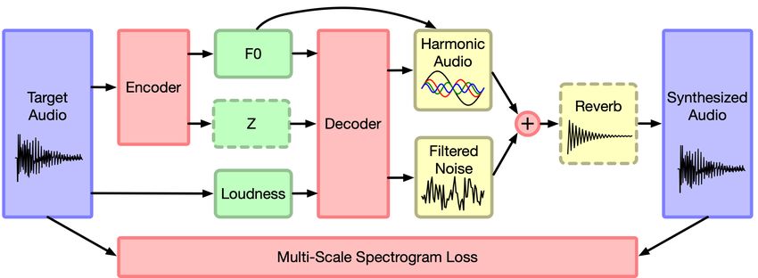
Published as a conference paper at ICLR 2020

this with a smoothed amplitude envelope by adding overlapping Hamming windows at the center of
each frame and scaled by the amplitude. For these experiments we found a 4ms (64 timesteps) hop
size and 8 ms frame size (50% overlap) to be responsive to changes while removing artifacts.

3.4   F ILTER D ESIGN : F REQUENCY S AMPLING M ETHOD

Linear filter design is a cornerstone of many DSP techniques. Standard convolutional layers are
equivalent to linear time invariant finite impulse response (LTI-FIR) filters. However, to ensure
interpretability and prevent phase distortion, we employ the frequency sampling method to convert
network outputs into impulse responses of linear-phase filters.
Here, we design a neural network to predict the frequency-domain transfer functions of a FIR filter
for every output frame. In particular, the neural network outputs a vector Hl (and accordingly
hl = IDFT(Hl )) for the l-th frame of the output. We interpret Hl as the frequency-domain transfer
function of the corresponding FIR filter. We therefore implement a time-varying FIR filter.
To apply the time-varying FIR filter to the input, we divide the audio into non-overlapping frames xl
to match the impulse responses hl . We then perform frame-wise convolution via multiplication of
frames in the Fourier domain: Yl = Hl Xl where Xl = DFT(xl ) and Yl = DFT(yl ) is the output.
We recover the frame-wise filtered audio, yl = IDFT(Yl ), and then overlap-add the resulting frames
with the same hop size and rectangular window used to originally divide the input audio. The hop
size is given by dividing the audio into equally spaced frames for each frame of conditioning. For
64000 samples and 250 frames, this corresponds to a hop size of 256.
In practice, we do not use the neural network output directly as Hl . Instead, we apply a window
function W on the network output to compute Hl . The shape and size of the window can be decided
independently to control the time-frequency resolution trade-off of the filter. In our experiments, we
default to a Hann window of size 257. Without a window, the resolution implicitly defaults to a
rectangular window which is not ideal for many cases. We take care to shift the IR to zero-phase
(symmetric) form before applying the window and revert to causal form before applying the filter.

3.5   F ILTERED N OISE / S UBTRACTIVE S YNTHESIZER

Natural sounds contain both harmonic and stochastic components. The Harmonic plus Noise model
captures this by combining the output of an additive synthesizer with a stream of filtered noise (Serra
& Smith, 1990; Beauchamp, 2007). We are able to realize a differentiable filtered noise synthesizer
by simply applying the LTV-FIR filter from above to a stream of uniform noise Yl = Hl Nl where
Nl is the IDFT of uniform noise in domain [-1, 1].

3.6   R EVERB : L ONG IMPULSE RESPONSES

Room reverbation (reverb) is an essential characteristic of realistic audio, which is usually implicitly
modeled by neural synthesis algorithms. In contrast, we gain interpretability by explicitly factoriz-
ing the room acoustics into a post-synthesis convolution step. A realistic room impulse response
(IR) can be as long as several seconds, corresponding to extremely long convolutional kernel sizes
(∼10-100k timesteps). Convolution via matrix multiplication scales as O(n3 ), which is intractable
for such large kernel sizes. Instead, we implement reverb by explicitly performing convolution as
multiplication in the frequency domain, which scales as O(n log n) and does not bottleneck training.

4     E XPERIMENTS

For empirical verification of this approach, we test two DDSP autoencoder variants–supervised and
unsupervised–on two different musical datasets: NSynth (Engel et al., 2017) and a collection of solo
violin performances. The supervised DDSP autoencoder is conditioned on fundamental frequency
(F0) and loudness features extracted from audio, while the unsupervised DDSP autoencoder learns
F0 jointly with the rest of the network.

                                                   5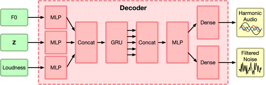
Published as a conference paper at ICLR 2020

Figure 2: Autoencoder architecture. Red components are part of the neural network architecture,
green components are the latent representation, and yellow components are deterministic synthesiz-
ers and effects. Components with dashed borders are not used in all of our experiments. Namely,
z is not used in the model trained on solo violin, and reverb is not used in the models trained on
NSynth. See the appendix for more detailed diagrams of the neural network components.

4.1   DDSP AUTOENCODER

DDSP components do not put constraints on the choice of generative model (GAN, VAE, Flow, etc.),
but we focus here on a deterministic autoencoder to investigate the strength of DDSP components
independent of any particular approach to adversarial training, variational inference, or Jacobian
design. Just as autoencoders utilizing convolutional layers outperform fully-connected autoencoders
on images, we find DDSP components are able to dramatically improve autoencoder performance
in the audio domain. Introducing stochastic latents (such as in GAN, VAE, and Flow models) will
likely further improve performance, but we leave that to future work as it is orthogonal to the core
question of DDSP component performance that we investigate in this paper.
In a standard autoencoder, an encoder network fenc (·) maps the input x to a latent representation
z = fenc (x) and a decoder network fdec (·) attempts to directly reconstruct the input x̂ = fdec (z).
Our architecture (Figure 2) contrasts with this approach through the use of DDSP components and
a decomposed latent representation.
Encoders: Detailed descriptions of the encoders are given in Section B.1. For the supervised au-
toencoder, the loudness l(t) is extracted directly from the audio, a pretrained CREPE model with
fixed weights (Kim et al., 2018) is used as an f (t) encoder to extact the fundamental frequency, and
optional encoder extracts a time-varying latent encoding z(t) of the residual information. For the
z(t) encoder, MFCC coefficients (30 per a frame) are first extracted from the audio, which corre-
spond to the smoothed spectral envelope of harmonics (Beauchamp, 2007), and transformed by a
single GRU layer into 16 latent variables per a frame.
For the unsupervised autoencoder, the pretrained CREPE model is replaced with a Resnet architec-
ture (He et al., 2016) that extracts f (t) from a mel-scaled log spectrogram of the audio, and is jointly
trained with the rest of the network.
Decoder: A detailed description of the decoder network is given in Section B.2. The decoder
network maps the tuple (f (t), l(t), z(t)) to control parameters for the additive and filtered noise
synthesizers described in Section 3. The synthesizers generate audio based on these parameters, and
a reconstruction loss between the synthesized and original audio is minimized. The network archi-
tecture is chosen to be fairly generic (fully connected, with a single recurrent layer) to demonstrate
that it is the DDSP components, and not other modeling decisions, that enables the quality of the
work.
Also unique to our approach, the latent f (t) is fed directly to the additive synthesizer as it has
structural meaning for the synthesizer outside the context of any given dataset. As shown later in
Section 5.2, this disentangled representation enables the model to both interpolate within and ex-

                                                   6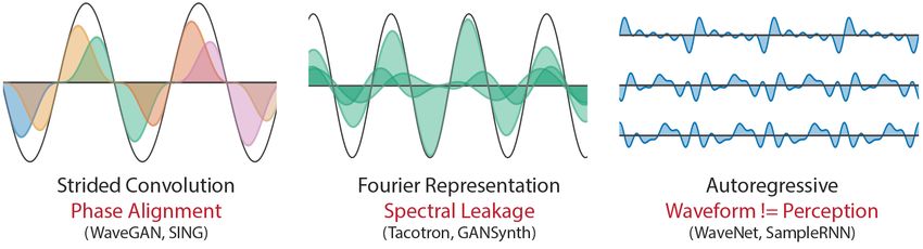
Published as a conference paper at ICLR 2020

                                                    Loudness (L1 )     F0 (L1 )    F0 Outliers
          Supervised
          WaveRNN (Hantrakul et al., 2019)                0.10           1.00           0.07
          DDSP Autoencoder                                0.07           0.02          0.003
          Unsupervised
          DDSP Autoencoder                                0.09           0.80           0.04

Table 1: Resynthesis accuracies. Comparison of DDSP models to SOTA WaveRNN model provided
the same conditioning information. The supervised DDSP Autoencoder and WaveRNN models
use the fundamental frequency from a pretrained CREPE model, while the unsupervised DDSP
autoencoder learns to infer the frequency from the audio during training.

trapolate outside the data distribution. Indeed, recent work support incorporation of strong inductive
biases as a prerequisite for learning disentangled representations (Locatello et al., 2018).
Model Size: Table B.6, compares parameter counts for the DDSP models and comparable mod-
els including GANSynth (Engel et al., 2019), WaveRNN (Hantrakul et al., 2019), and a WaveNet
Autoencoder (Engel et al., 2017). The DDSP models have the fewest parameters (up to 10 times
less), despite no effort to minimize the model size in these experiments. Initial experiments with
very small models (240k parameters, 300x smaller than a WaveNet Autoencoder) have less realistic
outputs than the full models, but still have fairly high quality and are promising for low-latency
applications, even on CPU or embedded devices. Audio samples are available in the online supple-
ment2 .

4.2     DATASETS

NSynth: We focus on a smaller subset of the NSynth dataset (Engel et al., 2017) consistent with
other work (Engel et al., 2019; Hantrakul et al., 2019). It totals 70,379 examples comprised mostly
of strings, brass, woodwinds and mallets with pitch labels within MIDI pitch range 24-84. We
employ a 80/20 train/test split shuffling across instrument families. For the NSynth experiments,
we use the autoencoder as described above (with the z(t) encoder). We experiment with both the
supervised and unsupervised variants.
Solo Violin: The NSynth dataset does not capture aspects of a real musical performance. Using
the MusOpen royalty free music library, we collected 13 minutes of expressive, solo violin perfor-
mances4 . We purposefully selected pieces from a single performer (John Garner), that were mono-
phonic and shared a consistent room environment to encourage the model to focus on performance.
Like NSynth, audio is converted to mono 16kHz and divided into 4 second training examples (64000
samples total). Code to process the audio files into a dataset is available online.5
For the solo violin experiments, we use the supervised variant of the autoencoder (without the z(t)
encoder), and add a reverb module to the signal processor chain to account for room reverberation.
While the room impulse response could be produced as an output of the decoder, given that the solo
violin dataset has a single acoustic environment, we use a single fixed variable (4 second reverb
corresponding to 64000 dimensions) for the impulse response.

4.2.1    M ULTI - SCALE SPECTRAL LOSS

The primary objective of the autoencoder is to minimize reconstruction loss. However, for audio
waveforms, point-wise loss on the raw waveform is not ideal, as two perceptually identical audio
samples may have distinct waveforms, and point-wise similar waveforms may sound very different.
Instead, we use a multi-scale spectral loss–similar to the multi-resolution spectral amplitude distance
in Wang et al. (2019)–defined as follows. Given the original and synthesized audio, we compute their
(magnitude) spectrogram Si and Ŝi , respectively, with a given FFT size i, and define the loss as the

  4
    Five pieces by John Garner (II. Double, III. Corrente, IV. Double Presto, VI. Double, VIII. Double) from
https://musopen.org/music/13574-violin-partita-no-1-bwv-1002/
  5
    https://github.com/magenta/ddsp

                                                     7
Published as a conference paper at ICLR 2020
Figure 3: Separate interpolations over loudness, pitch, and timbre. The conditioning features (solid
lines) are extracted from two notes and linearly mixed (dark to light coloring). The features of the
resynthsized audio (dashed lines) closely follow the conditioning. On the right, the latent vectors,
z(t), are interpolated, and the spectral centroid of resulting audio (thin solid lines) smoothly varies
between the original samples (dark solid lines).
sum of the L1 difference between Si and Ŝi as well as the L1 difference between log Si and log Ŝi .
Li = ||Si − Ŝi ||1 + α|| log Si − log Ŝi ||1 . (4)
where α is a weighting term set to 1.0 in our P experiments. The total reconstruction loss is then the
sum of all the spectral losses, Lreconstruction = i Li . In our experiments, we used FFT sizes (2048,
1024, 512, 256, 128, 64), and the neighboring frames in the Short-Time Fourier Transform (STFT)
overlap by 75%. Therefore, the Li ’s cover differences between the original and synthesized audios
at different spatial-temporal resolutions.
5 R ESULTS
5.1 H IGH - FIDELITY S YNTHESIS
As shown in Figure 5, the DDSP autoencoder learns to very accurately resynthesize the solo violin
dataset. Again, we highly encourage readers to listen to the samples provided in the online supple-
ment2 . A full decomposition of the components is provided Figure 5. High-quality neural audio
synthesis has previously required very large autoregressive models (Oord et al., 2016; Kalchbrenner
et al., 2018) or adversarial loss functions (Engel et al., 2019). While amenable to an adversarial loss,
the DDSP autoencoder achieves these results with a straightforward L1 spectrogram loss, a small
amount of data, and a relatively simple model. This demonstrates that the model is able to efficiently
exploit the bias of the DSP components, while not losing the expressive power of neural networks.
For the NSynth dataset, we quantitatively compare the quality of DDSP resynthesis with that of
a state-of-the-art baseline using WaveRNN (Hantrakul et al., 2019). The models are comparable
as they are trained on the same data, provided the same conditioning, and both targeted towards
realtime synthesis applications. In Table 1, we compute loudness and fundamental frequency (F0)
L1 metrics described in Section C of the appendix. Despite the strong performance of the baseline,
the supervised DDSP autoencoder still outperforms it, especially in F0 L1 . This is not unexpected,
as the additive synthesizer directly uses the conditioning frequency to synthesize audio.
The unsupervised DDSP autoencoder must learn to infer its own F0 conditioning signal directly
from the audio. As described in Section B.4, we improve optimization by also adding a perceptual
loss in the form of a pretrained CREPE network (Kim et al., 2018). While not as accurate as the
supervised DDSP version, the model does a fair job at learning to generate sounds with the correct
frequencies without supervision, outperforming the supervised WaveRNN model.
5.2 I NDEPENDENT C ONTROL OF L OUDNESS AND P ITCH
Interpolation: Interpretable structure allows for independent control over generative factors. Each
component of the factorized latent variables (f (t), l(t), z(t)) independently alters samples along a
matching perceptual axis. For example, Figure 3 shows an interpolation between two sound in the
loudness conditioning l(t). With other variables held constant, loudness of the synthesized audio
closely matches the interpolated input. Similarly, the model reliably matches intermediate pitches
between a high pitched f (t) and low pitched f (t). In Table C.2 of the appendix, we quantitatively
demonstrate how across interpolations, conditioning independently controls the corresponding char-
acteristics of the audio.
8Published as a conference paper at ICLR 2020
Figure 4: Timbre transfer from singing voice to violin. F0 and loudness features are extracted from
the voice and resynthesized with a DDSP autoencoder trained on solo violin.
With loudness and pitch explicitly controlled by (f (t), l(t)), the model should use the residual z(t)
to encode timbre. Although architecture and training do not strictly enforce this encoding, we qual-
itatively demonstrate how varying z leads to a smooth change in timbre. In Figure 3, we use the
smooth shift in spectral centroid, or “center of mass” of a spectrum, to illustrate this behavior.
Extrapolation: As described in Section 4.1, f (t) directly controls the additive synthesizer and
has structural meaning outside the context of any given dataset. Beyond interpolating between
datapoints, the model can extrapolate to new conditions not seen during training. The rightmost
plot of Figure 7 demonstrates this by resynthesizing a clip of solo violin after shifting f (t) down
an octave and outside the range of the training data. The audio remains coherent and resembles a
related instrument such as a cello. f (t) is only modified for the synthesizer, as the decoder is still
bounded by the nearby distribution of the training data and produces unrealistic harmonic content if
conditioned far outside that distribution.
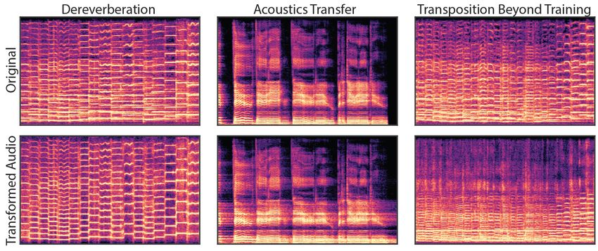
5.3 D EREVERBERATION AND ACOUSTIC T RANSFER
Removing reverb in a “blind” setting, where only reverberated audio is available, is a standing
problem in acoustics (Naylor & Gaubitch, 2010). However, a benefit of our modular approach to
generative modeling is that it becomes possible to completely separate the source audio from the
effect of the room. For the solo violin dataset, the DDSP autoencoder is trained with an additional
reverb module as shown in Figure 2 and described in Section 3.6. Figure 7 (left) demonstrates that
bypassing the reverb module during resynthesis results in completely dereverberated audio, similar
to recording in an anechoic chamber. The quality of the approach is limited by the underlying
generative model, which is quite high for our autoencoder. Similarly, Figure 7 (center) demonstrates
that we can also apply the learned reverb model to new audio, in this case singing, and effectively
transfer the acoustic environment of the solo violin recordings.
5.4 T IMBRE T RANSFER
Figure 4 demonstrates timbre transfer, converting the singing voice of an author into a violin. F0 and
loudness features are extracted from the singing voice and the DDSP autoencoder trained on solo
violin used for resynthesis. To better match the conditioning features, we first shift the fundamental
frequency of the singing up by two octaves to fit a violin’s typical register. Next, we transfer the
room acoustics of the violin recording (as described in Section 5.3) to the voice before extracting
loudness, to better match the loudness contours of the violin recordings. The resulting audio captures
many subtleties of the singing with the timbre and room acoustics of the violin dataset. Note the
interesting “breathing” artifacts in the silence corresponding to unvoiced syllables from the singing.
6 C ONCLUSION
The DDSP library fuses classical DSP with deep learning, providing the ability to take advantage
of strong inductive biases without losing the expressive power of neural networks and end-to-end
9Published as a conference paper at ICLR 2020
learning. We encourage contributions from domain experts and look forward to expanding the scope
of the DDSP library to a wide range of future applications.
R EFERENCES
S. O. Arik, H. Jun, and G. Diamos. Fast spectrogram inversion using multi-head convolutional
neural networks. IEEE Signal Processing Letters, 26(1):94–98, Jan 2019. doi: 10.1109/LSP.
2018.2880284.
James W Beauchamp. Analysis, synthesis, and perception of musical sounds. Springer, 2007.
Merlijn Blaauw and Jordi Bonada. A neural parametric singing synthesizer modeling timbre and
expression from natural songs. Applied Sciences, 7(12):1313, 2017.
Pritish Chandna, Merlijn Blaauw, Jordi Bonada, and Emilia Gomez. Wgansing: A multi-voice
singing voice synthesizer based on the wasserstein-gan. arXiv preprint arXiv:1903.10729, 2019.
Taishih Chi, Powen Ru, and Shihab A Shamma. Multiresolution spectrotemporal analysis of com-
plex sounds. The Journal of the Acoustical Society of America, 118(2):887–906, 2005.
Alexandre Defossez, Neil Zeghidour, Nicolas Usunier, Leon Bottou, and Francis Bach. Sing:
Symbol-to-instrument neural generator. In S. Bengio, H. Wallach, H. Larochelle, K. Grauman,
N. Cesa-Bianchi, and R. Garnett (eds.), Advances in Neural Information Processing Systems 31,
pp. 9041–9051. Curran Associates, Inc., 2018. URL http://papers.nips.cc/paper/
8118-sing-symbol-to-instrument-neural-generator.pdf.
Chris Donahue, Julian McAuley, and Miller Puckette. Adversarial audio synthesis. In International
Conference on Learning Representations, 2019. URL https://openreview.net/forum?
id=ByMVTsR5KQ.
Alexey Dosovitskiy and Thomas Brox. Generating images with perceptual similarity metrics based
on deep networks. In Advances in neural information processing systems, pp. 658–666, 2016.
Jesse Engel, Cinjon Resnick, Adam Roberts, Sander Dieleman, Douglas Eck, Karen Simonyan, and
Mohammad Norouzi. Neural audio synthesis of musical notes with WaveNet autoencoders. In
ICML, 2017.
Jesse Engel, Kumar Krishna Agrawal, Shuo Chen, Ishaan Gulrajani, Chris Donahue, and Adam
Roberts. GANSynth: Adversarial neural audio synthesis. In International Conference on Learn-
ing Representations, 2019. URL https://openreview.net/forum?id=H1xQVn09FX.
Philippe Esling, Naotake Masuda, Adrien Bardet, Romeo Despres, et al. Universal audio synthesizer
control with normalizing flows. arXiv preprint arXiv:1907.00971, 2019.
James L Flanagan. Speech analysis synthesis and perception, volume 3. Springer Science & Busi-
ness Media, 2013.
David Ha and Jürgen Schmidhuber. World models. arXiv preprint arXiv:1803.10122, 2018.
Lamtharn (Hanoi) Hantrakul, Jesse Engel, Adam Roberts, and Chenjie Gu. Fast and flexible neural
audio synthesis. In ISMIR, 2019.
Kaiming He, Xiangyu Zhang, Shaoqing Ren, and Jian Sun. Deep residual learning for image recog-
nition. In Proceedings of the IEEE conference on computer vision and pattern recognition, pp.
770–778, 2016.
Matthew D Hoffman and Perry R Cook. Feature-based synthesis: Mapping acoustic and perceptual
features onto synthesis parameters. In ICMC. Citeseer, 2006.
Kurt Hornik, Maxwell Stinchcombe, and Halbert White. Multilayer feedforward networks are uni-
versal approximators. Neural networks, 2(5):359–366, 1989.
10Published as a conference paper at ICLR 2020
Cheng-Zhi Anna Huang, David Duvenaud, Kenneth C Arnold, Brenton Partridge, Josiah W Ober-
holtzer, and Krzysztof Z Gajos. Active learning of intuitive control knobs for synthesizers using
gaussian processes. In Proceedings of the 19th international conference on Intelligent User In-
terfaces, pp. 115–124. ACM, 2014.
Nal Kalchbrenner, Erich Elsen, Karen Simonyan, Seb Noury, Norman Casagrande, Edward Lock-
hart, Florian Stimberg, Aaron van den Oord, Sander Dieleman, and Koray Kavukcuoglu. Efficient
neural audio synthesis. arXiv preprint arXiv:1802.08435, 2018.
Jong Wook Kim, Justin Salamon, Peter Li, and Juan Pablo Bello. Crepe: A convolutional repre-
sentation for pitch estimation. In 2018 IEEE International Conference on Acoustics, Speech and
Signal Processing (ICASSP), pp. 161–165. IEEE, 2018.
Anssi Klapuri, Tuomas Virtanen, and Jan-Markus Holm. Robust multipitch estimation for the anal-
ysis and manipulation of polyphonic musical signals. In Proc. COST-G6 Conference on Digital
Audio Effects, pp. 233–236, 2000.
Y. LeCun, B. Boser, J. S. Denker, D. Henderson, R. E. Howard, W. Hubbard, and L. D. Jackel.
Backpropagation applied to handwritten zip code recognition. Neural Computation, 1(4):541–
551, 1989. doi: 10.1162/neco.1989.1.4.541. URL https://doi.org/10.1162/neco.
1989.1.4.541.
Francesco Locatello, Stefan Bauer, Mario Lucic, Sylvain Gelly, Bernhard Schölkopf, and Olivier
Bachem. Challenging common assumptions in the unsupervised learning of disentangled repre-
sentations. arXiv preprint arXiv:1811.12359, 2018.
Robert McAulay and Thomas Quatieri. Speech analysis/synthesis based on a sinusoidal representa-
tion. IEEE Transactions on Acoustics, Speech, and Signal Processing, 34(4):744–754, 1986.
Soroush Mehri, Kundan Kumar, Ishaan Gulrajani, Rithesh Kumar, Shubham Jain, Jose Sotelo,
Aaron Courville, and Yoshua Bengio. Samplernn: An unconditional end-to-end neural audio
generation model. arXiv preprint arXiv:1612.07837, 2016.
Michelle Moerel, Federico De Martino, and Elia Formisano. Processing of natural sounds in human
auditory cortex: tonotopy, spectral tuning, and relation to voice sensitivity. Journal of Neuro-
science, 32(41):14205–14216, 2012.
Masanori Morise, Fumiya Yokomori, and Kenji Ozawa. World: a vocoder-based high-quality speech
synthesis system for real-time applications. IEICE TRANSACTIONS on Information and Systems,
99(7):1877–1884, 2016.
Patrick A Naylor and Nikolay D Gaubitch. Speech dereverberation. Springer Science & Business
Media, 2010.
Aaron van den Oord, Sander Dieleman, Heiga Zen, Karen Simonyan, Oriol Vinyals, Alex Graves,
Nal Kalchbrenner, Andrew Senior, and Koray Kavukcuoglu. Wavenet: A generative model for
raw audio. arXiv preprint arXiv:1609.03499, 2016.
Heiko Purnhagen and Nikolaus Meine. Hiln-the mpeg-4 parametric audio coding tools. In 2000
IEEE International Symposium on Circuits and Systems. Emerging Technologies for the 21st Cen-
tury. Proceedings (IEEE Cat No. 00CH36353), volume 3, pp. 201–204. IEEE, 2000.
Xavier Serra and Julius Smith. Spectral modeling synthesis: A sound analysis/synthesis system
based on a deterministic plus stochastic decomposition. Computer Music Journal, 14(4):12–24,
1990.
Julius Orion Smith. Physical audio signal processing: For virtual musical instruments and audio
effects. W3K publishing, 2010.
Ilya Sutskever, Oriol Vinyals, and Quoc V Le. Sequence to sequence learning with neural networks.
In Advances in neural information processing systems, pp. 3104–3112, 2014.
Edwin Tellman, Lippold Haken, and Bryan Holloway. Timbre morphing of sounds with unequal
numbers of features. Journal of the Audio Engineering Society, 43(9):678–689, 1995.
11Published as a conference paper at ICLR 2020
Frédéric E Theunissen and Julie E Elie. Neural processing of natural sounds. Nature Reviews
Neuroscience, 15(6):355, 2014.
Ashish Vaswani, Noam Shazeer, Niki Parmar, Jakob Uszkoreit, Llion Jones, Aidan N Gomez,
Łukasz Kaiser, and Illia Polosukhin. Attention is all you need. In Advances in neural information
processing systems, pp. 5998–6008, 2017.
Xin Wang, Shinji Takaki, and Junichi Yamagishi. Neural source-filter waveform models for statisti-
cal parametric speech synthesis. arXiv preprint arXiv:1904.12088, 2019.
Yuxuan Wang, RJ Skerry-Ryan, Daisy Stanton, Yonghui Wu, Ron J Weiss, Navdeep Jaitly,
Zongheng Yang, Ying Xiao, Zhifeng Chen, Samy Bengio, et al. Tacotron: Towards end-to-end
speech synthesis. In INTERSPEECH, 2017.
P. J. Werbos. Backpropagation through time: what it does and how to do it. Proceedings of the
IEEE, 78(10):1550–1560, Oct 1990. doi: 10.1109/5.58337.
Ronald J Williams and David Zipser. Gradient-based learning algorithms for recurrent connection-
ist networks. College of Computer Science, Northeastern University Boston, MA, 1990.
12Published as a conference paper at ICLR 2020
A A PPENDIX
Figure 5: Decomposition of a clip of solo violin. Audio is visualized with log magnitude spec-
trograms. Loudness and fundamental frequency signals are extracted from the original audio. The
loudness curve does not exhibit clear note segmentations because of the effects of the room acous-
tics. The DDSP autoencoder takes those conditioning signals and predicts amplitudes, harmonic
distributions, and noise magnitudes. Note that the amplitudes are clearly segmented along note
boundaries without supervision and that the harmonic and noise distributions are complex and dy-
namic despite the simple conditioning signals. Finally, the extracted impulse response is applied to
the combined audio from the synthesizers to give the full resynthesis audio.
13Published as a conference paper at ICLR 2020
Figure 6: Diagram of the Additive Synthesizer component. The synthesizer generates audio as a sum
of sinusoids at harmonic (integer) multiples of the fundamental frequency. The neural network is
then tasked with emitting time-varying synthesizer parameters (fundamental frequency, amplitude,
harmonic distribution). In this example linear-frequency log-magnitude spectrograms show how
the harmonics initially follow the frequency contours of the fundamental. We then factorize the
harmonic amplitudes into an overall amplitude envelope that controls the loudness, and a normalized
distribution among the different harmonics that determines spectral variations.
Figure 7: Interpretable generative models enables disentanglement and extrapolation. Spectrograms
of audio examples include dereverberation of a clip of solo violin playing (left), transfer of the
extracted room response to new audio (center), and transposition below the range of training data
(right).
B M ODEL DETAILS
B.1 E NCODERS
The model has three encoders: f -encoder that outputs fundamental frequency f (t), l-encoder that
outputs loudness l(t), and a z-encoder that outputs residual vector z(t).
f -encoder: We use a pretrained CREPE pitch detector (Kim et al., 2018) as the f -encoder to extract
ground truth fundamental frequencies (F0) from the audio. We used the “large” variant of CREPE,
which has SOTA accuracy for monophonic audio samples of musical instruments. For our super-
vised autoencoder experiments, we fixed the weights of the f -encoder like (Hantrakul et al., 2019),
and for our unsupervised autoencoder experiemnts we jointly learn the weights of a resnet model
fed log mel spectrograms of the audio. Full details of the resnet architecture are show in Table 2.
14Published as a conference paper at ICLR 2020
l-encoder: We use identical computational steps to extract loudness as (Hantrakul et al., 2019).
Namely, an A-weighting of the power spectrum, which puts greater emphasis on higher frequencies,
followed by log scaling. The vector is then centered according to the mean and standard deviation
of the dataset.
z-encoder: As shown in Figure 8, the encoder first calculates MFCC’s (Mel Frequency Cepstrum
Coefficients) from the audio. MFCC is computed from the log-mel-spectrogram of the audio with
a FFT size of 1024, 128 bins of frequency range between 20Hz to 8000Hz, overlap of 75%. We
use only the first 30 MFCCs that correspond to a smoothed spectral envelope. The MFCCs are then
passed through a normalization layer (which has learnable shift and scale parameters) and a 512-unit
GRU. The GRU outputs (over time) fed to a 512-unit linear layer to obtain z(t). The z embedding
reported in this model has 16 dimensions across 250 time-steps.
Residual Block Output Size kT ime kF req sF req kF ilters
layer norm + relu - - - - -
conv - 1 1 1 kF ilters / 4
layer norm + relu - - - - -
conv - 3 3 sF req kF ilters / 4
layer norm + relu - - - - -
conv - 1 1 1 kF ilters
add residual - - - - -
Resnet Output Size kT ime kF req sF req kF ilters
LogMelSpectrogram (125, 229, 1) - - - -
conv2d (125, 115, 64) 7 7 2 64
max pool (125, 58, 64) 1 3 2 -
residual block (125, 58, 128) 3 3 1 128
residual block (125, 57, 128) 3 3 1 128
residual block (125, 29, 256) 3 3 2 256
residual block (125, 29, 256) 3 3 1 256
residual block (125, 29, 256) 3 3 1 256
residual block (125, 15, 512) 3 3 2 512
residual block (125, 15, 512) 3 3 1 512
residual block (125, 15, 512) 3 3 1 512
residual block (125, 15, 512) 3 3 1 512
residual block (125, 8, 1024) 3 3 2 1024
residual block (125, 8, 1024) 3 3 1 1024
residual block (125, 8, 1024) 3 3 1 1024
dense (125, 1, 128) - - 128 1
upsample time (1000, 1, 128) - - - -
softplus and normalize (1000, 1, 128) - - - -
Table 2: Model architecture for the f(t) encoder using a Resnet on log mel spectrograms. Spectro-
grams have a frame size of 2048 and a hop size of 512, and are upsampled at the end to have the
same time resoultion as other latents (4ms per a frame). All convolutions use “same” padding and
a temporal stride of 1. Each residual block uses a bottleneck structure (He et al., 2016). The final
output is a normalized probablity distribution over 128 frequency values (logarithmically scaled be-
tween 8.2Hz and 13.3kHz (https://www.inspiredacoustics.com/en/MIDI_note_
numbers_and_center_frequencies)). The finally frequency value is the weighted sum of
each frequency by its probability.
B.2 D ECODER
The decoder’s input is the latent tuple (f (t), l(t), z(t)) (250 timesteps). Its outputs are the parame-
ters required by the synthesizers. For example, in the case of the harmonic synthesizer and filtered
noise synthesizer setup, the decoder outputs a(t) (amplitudes of the harmonics) for the harmonic
synthesizer (note that f (t) is fed directly from the latent), and H (transfer function of the FIR filter)
for the filtered noise synthesizer.
15Published as a conference paper at ICLR 2020
Figure 8: Diagram of the z-encoder.
As shown in Figure 9, we use a “shared-bottom” architecture, which computes a shared embedding
from the latent tuple, and then have one head for each of the (a(t), H) outputs.
In particular, we apply separate MLPs to each of the (f (t), l(t), z(t)) input. The outputs of the
MLPs are concatenated and passed to a 512-unit GRU. We concatenate the GRU outputs with the
outputs of the f (t) and l(t) MLPs (in the channel dimenssion) and pass it through a final MLP and
Linear layer to get the decoder outputs.
Figure 9: Diagram of the decoder for the harmonic synthesizer and the filtered noise synthesizer.
The MLP architecture, shown in Figure 10, is a standard MLP with a layer normalization
(tf.contrib.layers.layer_norm ) before the RELU nonlinearity. In Figure 9, all the
MLPs have 3 layers and each layer has 512 units.
Figure 10: MLP in the decoder.
B.3 T RAINING
Because all DDSP components are differentiable, the model is differentiable end-to-end. Therefore,
we can apply any SGD optimizer to train the model. We used ADAM optimizer with learning rate
0.001 and exponential learning rate decay 0.98 every 10,000 steps.
16Published as a conference paper at ICLR 2020
B.4 P ERCEPTUAL LOSS
To help guide the DDSP autoencoder that must predict f (t) on the NSynth dataset, we also added
an additional perceptual loss using pretrained models, such as the CREPE (Kim et al., 2018) pitch
estimator and the encoder of the WaveNet autoencoder (Engel et al., 2017). Compared to the L1
loss on the spectrogram, the activations of different layers in these models correlate better with the
perceptual quality of the audio. After a large-scale hyperparameter search, we obtained our best
results by using the L1 distance between the activations of the small CREPE model’s fifth max pool
layer with a weighting of 5 × 10⁻⁵ relative to the spectral loss.
B.5 S YNTHESIZERS
Harmonic synthesizer / Additive Synthesis: We use 101 harmonics in the harmonic synthesizer
(i.e., a(t)’s dimension is 101). Amplitude and harmonic distribution parameters are upsampled with
overlapping Hamming window envelopes whose frame size is 128 and hop size is 64. Initial phases
are all fixed to zero, as neither the spectrogram loss functions or human perception are sensitive
to absolute offsets in harmonic phase. We also do not include synthesis elements to model DC
components to signals as they are inaudible and not reflected in the spectrogram losses.
We force the amplitudes, harmonic distributions, and filtered noise magnitudes to be non-negative
by applying a sigmoid nonlinearity to network outputs. We find a slight improvement in traning
stability by modifying the sigmoid to have a scaled output, larger slope by exponentiating, and
threshold at a minimum value:
y = 2.0 · sigmoid(x)log 10 + 10−7 (5)
Filtered noise synthesizer: We use 65 network output channels as magnitude inputs to the FIR filter
of the filtered noise synthesizer.
B.6 PARAMETER C OUNTS
Model Parameters
WaveNet Autoencoder (Engel et al., 2017) 75M
WaveRNN (Hantrakul et al., 2019) 23M
GANSynth (Engel et al., 2019) 15M
DDSP Autoencoder (Unsupervised) 12M
DDSP Autoencoder (Supervised, NSynth) 7M
DDSP Autoencoder (Supervised, Solo Violin) 6M
DDSP Autoencoder Tiny (Supervised, Solo Violin) 0.24M
Table 3: Parameter counts for different models. All models trained on NSynth dataset except for
those marked (Solo Violin). Autoregressive models have the most parameters with GANs requiring
less. The DDSP models examined in this paper (which have not been optimized at all for size)
require 2 to 3 times less parameters than GANSynth. The unsupervised model has more parameters
because of the CREPE (small) f (t) encoder, and the autoencoder has additional parameters for the
z(t) encoder. Initial experiments with extremely small models (single GRU, 256 units), have slightly
less realistic outputs, but still relatively high quality (as can be heard in the supplemental audio).
C E VALUATION DETAILS
C.1 M ETRICS
Loudness L1 distance: The loudness vector is extracted from the synthesized audio and L1 dis-
tance computed against the input’s conditioning loudness vector (ground truth). A better model will
produce lower L1 distances, indicating input and generated loudness vectors closely match. Note
this distance is not back-propagated through the network as a training objective.
17Published as a conference paper at ICLR 2020
F0 L1 distance: The F0 L1 distance is reported in MIDI space for easier interpretation; an average
F0 L1 of 1.0 corresponds to a semitone difference. We use the same confidence threshold of 0.85
in (Hantrakul et al., 2019) to select portions where there was detectable pitch content, and compute
the metric only in these areas.
F0 Outliers: Pitch tracking using CREPE, like any pitch tracker, is not completely reliable. In-
stabilities in pitch tracking, such as sudden octave jumps at low volumes, can result errors not due
to model performance and need to be accounted for. F0 outliers accounts for pitch tracking imper-
fections in CREPE (Kim et al., 2018) vs. genuinely bad samples generated by the trained model.
CREPE outputs both an F0 value as well as a F0 confidence. Samples with confidences below a
threshold of 0.85 in (Hantrakul et al., 2019) are labeled as outliers and usually indicate the sample
was mostly noise with no pitch or harmonic component. As the model outputs better quality audio,
the number of outliers decrease, thus lower scores indicate better performance.
C.2 I NTERPOLATION M ETRICS
Loudness L1 and F0 L1 are shown for different interpolation tasks in table C.2. In reconstruc-
tion, the model is supplied with the standard (f (t)A , l(t)A , z(t)A ). Loudness (L1 ) and F0 (L1 )
are computed against the ground truth inputs. In loudness interpolation, the model is supplied
with (f (t)A , l(t)B , z(t)A ), and Loudness (L1 ) is calculated using l(t)B as ground truth instead
of (l(t)A ). For F0 interpolation, the model is supplied with (f (t)B , l(t)A , z(t)A ) and F0 (L1 ) is
calculated using f (t)B as ground truth instead of f (t)A . For Z interpolation, the model is supplied
with (f (t)A , l(t)A , z(t)B ). The low and constant Loudness (L1 ) and F0 (L1 ) metrics across these
interpolations indicate the model is able independently vary these variables without affecting other
components.
Task Loudness (L1 ) F0 (L1 )
Reconstruction 0.042 0.060
Loudness l(t) interp. 0.061 0.060
F0 f (t) interp. 0.048 0.070
Z z(t) interp. 0.063 0.065
Table 4: Loudness and F0 metrics for different interpolation tasks.
18Published as a conference paper at ICLR 2020
D OTHER NOTES
D.1 S INUSOIDAL MODELS
While unconstrained sinusoidal oscillator banks are strictly more expressive than harmonic oscil-
lators, we restricted ourselves to harmonic synthesizers for the time being to focus the problem
domain. However, this is not a fundamental limitation of the technique and perturbations such as
inharmonicity can also be incorporated to handle phenomena such as stiff strings (Smith, 2010).
D.2 R EGULARIZATION
It is worth mentioning that the modular structure of the synthesizers also makes it possible to define
additional losses in terms of different synthesizer outputs and parameters. For example, we may
impose an SNR loss to penalize outputs with too much noise if we know the training data consists
of mostly clean data. We have not experimented too much with such engineered losses, but we
believe they can make training more efficient, even though such engineering methods deviates from
the end-to-end training paradigm,
19You can also read