The Power of Helicopter Money Revisited: A New Keynesian Perspective - Bank of Canada

Staff Discussion Paper/Document d’analyse du personnel —
2020-01
Last updated: February 7, 2020

The Power of Helicopter
Money Revisited: A New
Keynesian Perspective
by Thomas J. Carter and Rhys R. Mendes

International Economic Analysis Department
Bank of Canada, Ottawa, Ontario, Canada K1A 0G9

tcarter@bankofcanada.ca, rmendes@bankofcanada.ca

Bank of Canada staff discussion papers are completed staff research studies on a wide variety of subjects relevant to
central bank policy, produced independently from the Bank’s Governing Council. This research may support or challenge
prevailing policy orthodoxy. Therefore, the views expressed in this paper are solely those of the authors and may differ
from official Bank of Canada views. No responsibility for them should be attributed to the Bank.
ISSN 1914-0568 ©2020 Bank of Canada

Page 1

Acknowledgements
We thank Robert Amano, José Dorich, Stefano Gnocchi and Sharon Kozicki for some
very useful comments and feedback on earlier versions of this discussion paper.

Page 2

Abstract
We analyze money financing of fiscal transfers (helicopter money) in two simple New
Keynesian models: a “textbook” model in which all money is non-interest-bearing
(e.g., all money is currency), and a more realistic model with interest-bearing
reserves. In the textbook model with only non-interest-bearing money, we find the
following:

• A money-financed fiscal expansion can be more stimulative than a debt-financed
 fiscal expansion of equal magnitude. However, the extra stimulus requires that
 the central bank abandon its usual feedback rule for an extended period, allowing
 interest rates to instead be determined by the rate of money creation.
• Moreover, the extra stimulus associated with money financing stems solely from
 its implications for the path of short-term interest rates and cannot be attributed
 to an oft-cited Ricardian-equivalence argument that money financing avoids the
 adverse wealth effects associated with higher taxes under debt financing.
• Because the stimulative effects of money financing are driven by its implications
 for interest rates, a combination of debt financing and sufficiently accommodative
 forward guidance can replicate all welfare-relevant outcomes while bypassing the
 potential political-economic complications associated with helicopter money.
• Apart from these complications, money financing also has the drawback that it
 would allow money-demand shocks to generate volatility in output and inflation,
 much as was the case under the money-targeting regimes of the 1970s and 1980s.
In the model with interest-bearing reserves, we find the following:

• The rate of money creation determines the interest rate on reserves, but broader
 interest rates are invariant across debt- and money-financing regimes.
• As a result, money financing delivers no extra stimulus relative to debt financing.
Overall, results suggest that helicopter money cannot be justified on the grounds that
it would allow policy-makers to get more stimulus out of a given fiscal expansion:
either money financing has no extra stimulative benefits to offer, or all potential
benefits could be pursued more effectively and robustly using alternative policies.
Topics: Credibility; Economic models; Fiscal policy; Inflation targets; Interest rates;
Monetary policy; Monetary policy framework; Transmission of monetary policy;
Uncertainty and monetary policy
JEL codes: E12, E41, E43, E51, E52, E58, E61, E63

Page 3

Résumé
Nous analysons le financement monétaire des transferts budgétaires (l’hélicoptère
monétaire) dans deux modèles simples de type néo-keynésien : un modèle classique
où la totalité de la monnaie ne porte pas intérêt, et un autre, plus réaliste, doté de
réserves portant intérêt. Dans le modèle classique, nous constatons ce qui suit :

• Une expansion budgétaire financée par l’émission de monnaie peut s’avérer plus
 accommodante qu’une expansion budgétaire de même ampleur financée par
 l’emprunt. Cela dit, l’expansion plus importante nécessite l’abandon par la banque
 centrale de sa règle de rétroaction habituelle durant une longue période, ce qui
 revient à laisser déterminer les taux d’intérêt par le rythme de création monétaire.
• En outre, l’expansion plus importante associée au financement monétaire
 découle uniquement de ses implications pour la trajectoire des taux d’intérêt à
 court terme. Elle ne peut pas être attribuée à l’argument souvent invoqué
 d’équivalence ricardienne, selon lequel le financement monétaire permet d’éviter
 les effets de richesse défavorables liés à la hausse des impôts qui accompagne le
 financement par l’emprunt.
• Étant donné que les effets expansionnistes du financement monétaire sont
 déterminés par les implications de ce dernier pour les taux d’intérêt, une
 combinaison de financement par l’emprunt et d’indications prospectives
 suffisamment accommodantes peut reproduire tous les résultats pertinents au
 regard du bien-être, tout en évitant les éventuelles complications politico-
 économiques associées à l’hélicoptère monétaire.
• Mis à part ces complications, le financement monétaire présente également
 l’inconvénient qu’il permettrait aux chocs de demande de monnaie d’engendrer
 une volatilité de la production et de l’inflation, comme c’était en grande partie le
 cas sous les régimes de ciblage monétaire des années 1970 et 1980.
Dans le modèle doté de réserves portant intérêt, nous constatons ce qui suit :

• Le rythme de création monétaire détermine le taux d’intérêt appliqué aux
 réserves, mais les taux d’intérêt en général sont invariants dans les régimes de
 financement par l’emprunt et de financement monétaire.
• Par conséquent, le financement monétaire ne génère pas d’expansion plus
 importante que le financement par l’emprunt.
Somme toute, nos résultats donnent à penser que l’hélicoptère monétaire ne peut se
justifier du fait qu’il permettrait aux décideurs publics de produire des effets
expansionnistes accrus grâce à une relance budgétaire donnée : soit le financement
monétaire n’offre pas d’avantages expansionnistes supplémentaires, soit tous les
avantages potentiels pourraient être obtenus à l’aide d’autres politiques de manière
plus efficace et robuste.

Page 4

Sujets : Crédibilité; Modèles économiques; Politique budgétaire; Cibles en matière
d’inflation; Taux d’intérêt; Politique monétaire; Cadre de la politique monétaire;
Transmission de la politique monétaire; Incertitude et politique monétaire
Codes JEL : E12, E41, E43, E51, E52, E58, E61, E63

1 Introduction
Milton Friedman (1969) first described a “helicopter drop” of money as a thought experiment to
demonstrate that governments should always be able to generate inflation. Recent years have
seen growing practical interest in helicopter money as a potential addition to the set of policy
tools available at the effective lower bound (ELB). Though exact definitions differ across the
literature, “helicopter money,” or “money financing,” 1 broadly refers to a combination of
monetary and fiscal policies under which expansionary fiscal measures are financed by creating
money rather than issuing debt. In this paper, we explore the mechanics and efficacy of these
policies in simple New Keynesian economies.
 Our analysis focuses mainly on understanding how the decision to finance a given fiscal
expansion using money creation might lead to different macroeconomic outcomes than would
occur were the same expansion financed using debt. Our results suggest that money financing,
when viewed through the lens of two simple New Keynesian models, cannot be justified on the
grounds that it would allow policy-makers to get more stimulus out of a given fiscal expansion.
More specifically, money financing should have no extra stimulative benefits relative to debt
financing when the money created takes the form of interest-bearing reserves. In contrast, if
money financing involves the creation of non-interesting-bearing money, then we find that it can
lead to additional stimulative benefits relative to debt financing. However, these stimulative
benefits could be replicated by combining a traditional debt-financed fiscal stimulus with a
commitment to a sufficiently accommodative interest rate path, implemented using forward
guidance or some other form of history-dependent monetary policy. As a consequence, the same
benefits could be achieved while side-stepping the potential political-economic complications
associated with helicopter money. We also highlight a significant risk that an unstable money-
demand curve might lead to greater aggregate volatility under money financing. This would make
it more difficult for policy-makers to gauge the amount of money financing needed to achieve a
given set of aggregate outcomes.
 That said, our results assume that the size of the fiscal expansion does not depend on the
mode of financing. This leaves open a possibility, emphasized by Bartsch et al. (2019) and several
others, that money financing could lead to larger (and potentially more timely) fiscal expansions.
We do not address such “extensive-margin” considerations in this paper. We also stress that our
findings are model-specific, though the models in question represent a workhorse framework
commonly used in academic and policy-making circles.
 While a full review of the literature lies outside the scope of this discussion paper, we briefly
note that Bernanke (2002, 2003) first rekindled interest in helicopter money in light of Japan’s
“lost decade,” while Buiter (2014) and Turner (2015) have recently argued for its addition to
policy-makers’ post-crisis tool kits. In particular, Turner (2015) argues that the technical case for

1
 The terms “(outright or overt) monetary financing,” “monetized fiscal action” and “money-financed fiscal program
(or stimulus)” are also sometimes used.

 1

money financing is sound and that appropriate institutional frameworks can be designed to
address the questions it raises concerning central banks’ independence from fiscal policy and
long-run commitment to price stability. Bartsch et al. (2019) outline one such framework in some
detail, namely a “standing emergency fiscal facility” that central banks could activate at the ELB
and then fund through money creation. Bernanke (2016) offers a broadly similar proposal.
 In contrast, Michael Woodford has argued that outcomes similar to those obtained under
money financing could be achieved while respecting the traditional separation of roles across
fiscal and monetary policy, assuming that the two sides operate under suitably complementary
frameworks. 2 At the same time, Borio and Zabai (2016), Kocherlakota (2016) and several others
have taken issue with the technical case for helicopter money. More specifically, they argue that
this case was first developed using models where money was assumed not to bear interest. In
contrast, they claim that the benefits of money financing may shrink—or even evaporate—in
real-world settings where money-financing would likely involve the creation of interest-bearing
reserves (“settlement balances” in the Canadian context).
 While all of the foregoing references rely on informal or partial-equilibrium arguments,
others have recently begun studying helicopter money in general-equilibrium New Keynesian
models. In particular, Galí (2019), English, Erceg and Lopez-Salido (2017) and Tsuruga and Wake
(2019) focus on models with non-interest-bearing money, while Harrison and Thomas (2019)
focus on the case of interest-bearing money. Many of our findings echo conclusions reached in
these studies. For example, English, Erceg and Lopez-Salido share our emphasis on the fact that
the benefits of helicopter money can be replicated by combining debt-financed fiscal stimulus
with an appropriate choice on the interest rate path. Similarly, Tsuruga and Wake share our
concerns about money financing’s vulnerability to instability in the money-demand curve.
 Since the general-equilibrium literature has focused mainly on settings where policy-makers
are assumed capable of permanently committing to money financing, one of our main
contributions is to shift attention to a more realistic setting in which the central bank eventually
reverts to setting its policies in line with a standard Taylor rule. In so doing, we find that the
duration of policy-makers’ commitment to money financing is a critical determinant of the
scheme’s overall efficacy: in the simple New Keynesian economies that we consider, significant
stimulative effects relative to debt financing can be achieved only if the central bank is prepared
to suspend its usual feedback rule for an extended period after the underlying fiscal stimulus has
passed. We also clarify the role that Ricardian equivalence plays in generating our results and
show that any extra stimulus associated with money financing cannot be attributed to an oft-
cited Ricardian-equivalence argument that money financing avoids the adverse wealth effects
associated with higher taxes under debt financing. This is because similar wealth effects also arise

2
 More specifically, Woodford argues that this could be done by combining a debt-financed fiscal
expansion with an appropriately designed nominal GDP target. See Reichlin, Turner and Woodford (2019),
along with Woodford (2012).

 2

under money financing due to the interest that households forego on savings allocated to money
rather than bonds.
 The remainder of this paper is organized as follows. Section 2 lays out a simple model in
which we maintain the common textbook assumption that money is a non-interest-bearing asset.
Section 3 then uses this model to explore the merits of money- versus debt-financed fiscal
expansions following large demand shocks, while Section 4 shifts attention to money-demand
shocks. We then discuss the role of Ricardian equivalence in Section 5 before introducing a simple
model with interest-bearing money in Section 6. In Section 7, we briefly discuss intermediate
cases where interest- and non-interest-bearing forms of money co-exist. Section 8 offers some
concluding remarks.

2 A textbook New Keynesian model
In this section, we lay out the simplest possible New Keynesian model that includes both money
and an ELB, maintaining the common textbook assumption that money is a non-interest-bearing
asset. To isolate the effects of the debt-financing versus money-financing decision, we assume
that the government’s spending choices are independent of the financing regime. In particular,
our simulations assume that the government responds to a large demand shock by temporarily
increasing its transfers to a representative household, with both the size and persistence of this
increase invariant to the financing decision.
 While Ricardian equivalence will imply that transfers of this sort should have no aggregate
effects under debt financing in the textbook model, our aim is to understand the incremental
stimulus provided by money financing over debt financing. As a result, the exact form of the
underlying fiscal expansion is not critical to our qualitative findings. For example, we would
obtain qualitatively similar results regarding the incremental effects of money financing if the
fiscal expansion took the form of an increase in government spending.

2.1 Private sector block
In our model, which is similar to those in English, Erceg and Lopez-Salido (2017) and Galí (2019),
the behaviour of the private sector is described by three standard equations. The first two are
the usual IS and Phillips curves, respectively: 3
 � = ( � +1 ) − ( ̂ − � +1 − ) (1)
and

3
 Both curves have been derived under the textbook assumption that real money balances enter the
household utility function on an additively separable basis. Additively separable preferences are a
common benchmark on which the New Keynesian literature often focuses. Moreover, Woodford (2003,
pp. 117–120 and 299–311) and Ireland (2004) argue that real money balance effects are weak enough
that assuming additively separable preferences is likely to provide a reasonable approximation in many
contexts.

 3

 � = � + ( � +1 ), (2)
where � denotes the output gap; 4 ̂ denotes the nominal interest rate, expressed as a deviation
from its steady-state value; 5 � +1 denotes inflation, expressed as a deviation from target; is a
demand shock; and ( , , ) are parameters.
 The third equation in the private sector block is a money-demand curve. This demand curve
captures the trade-off that households face when allocating funds between bonds, which pay
interest, and money, which generates a convenience yield but pays no interest and may involve
some storage costs. Specifically,
 = � − ̂ if ̂ > ̂ 
 
� � (3)
 ≥ � − ̂ if ̂ = ̂ ,

where � denotes real money balances, expressed as a deviation from steady state; 6 > 0 is a
parameter governing the rate at which the convenience yield falls as households allocate more
funds to money; and ̂ denotes an ELB at which money and bonds offer equal pecuniary
returns after taking storage costs into account (also expressed as a deviation from steady state).
Equation 3 states that households opt to hold money up to the point where the marginal dollar
generates a convenience yield just large enough to compensate for the interest rate that that
dollar would have earned if allocated to bonds, assuming that this rate exceeds the ELB. At the
ELB, there is no opportunity cost associated with holding money, so households are content to
hold any amount of money beyond a satiation level where the convenience yield is assumed to
become negligible. See Figure 1 for an illustration.

2.2 Policy block
To complete the model, the private sector block must be paired with a description of monetary
and fiscal policy. On this front, we begin with the consolidated government budget constraint
that arises after netting out transfers between the central bank and general government. Written
in deviations from steady state, this constraint reads as
 �
 � + (∆ ⁄ ) = (1 + ∗ ) � −1 + (1 + ∗ ) ∗ ( ̂ −1 − � ) + ̂ , (4)
 �
where � and (∆ ⁄ ) denote real debt held by the general public and real seigniorage revenue,
respectively, both expressed as deviations from their steady-state levels; 7 ∗ denotes the steady-

4
 That is, � ≡ log − log , where denotes output, while denotes the natural rate of output. In
this simple model, the latter coincides with steady-state output, so � can also be interpreted as the
percent deviation of output from its steady-state level.
5
 Specifically, ̂ ≡ ( − ∗ )/(1 + ∗ ), where denotes the nominal rate, and ∗ denotes the steady state
thereof. � has been defined analogously.
6
 More precisely, � ≡ log − log ∗ , where denotes real balances, and ∗ denotes the steady
state thereof.
7
 In particular, � ≡ ( − ∗ )/ ∗ , where denotes real debt, while ∗ and ∗ denote the steady-state
levels of real debt and real output, respectively. Both (∆ � ⁄ ) and ̂ have been defined analogously.

 4

state real interest rate; ∗ denotes the steady-state level of real debt; and ̂ denotes a real lump-
sum transfer to households, also expressed as a deviation from its steady-state level.
(Equivalently, − ̂ could be interpreted as a lump-sum tax). Transfers are assumed to obey a rule
of the form

 ̂ = − � −1 + , (5)
where is a shock meant to capture temporary discretionary transfers, while > 0 is a
parameter controlling the rate at which the government adjusts transfers to stabilize its bond
debt in the long run. Together, equations 4 and 5 stipulate that the government’s transfers,
principal and interest payments must be financed using some combination of seigniorage and
tax-backed bond issuance.
 Under the configuration of monetary and fiscal policy on which the New Keynesian literature
normally focuses, which we refer to as a “debt-financing regime,” debt issuance is assumed to
represent the consolidated government’s main financing margin. More specifically, the central
bank is assumed to set its policy rate according to a Taylor rule along the lines of

 ̂ = � ̂ , � + y � �, (6)

adjusting the money supply as needed to ensure that the money market reaches equilibrium at
the intended interest rate. Any seigniorage generated under this regime should thus be viewed
as a by-product of the central bank’s pursuit of an independent monetary policy, rather than a
deliberate effort to monetize some portion of the government’s transfers or principal or interest
payments. For this reason, fiscal authorities are assumed to stand ready to issue new debt as
needed to finance the portion of these outflows that seigniorage fails to cover.
 In contrast, the distinguishing feature of our “money-financing regime” is that monetary
policy is assumed to directly aim at providing the government with a certain amount of
seigniorage. While this goal can be modelled in several ways, we take an approach similar to that
of English, Erceg and Lopez-Salido (2017) in assuming that the central bank adjusts the money
supply as need to finance discretionary transfers—i.e., 8
 �
(∆ ⁄ ) = . (7)
In this case, the central bank no longer adjusts the money supply as needed to ratify an intended
value for the interest rate. Instead, monetary policy-makers must now adjust the interest rate as
needed to ensure that households are willing to hold the amount of money being created in

8
 An alternative approach would be to follow Galí (2019) in assuming a seigniorage target of the form
 �
(∆ ⁄ ) = ∗ � −1 + (1 + ∗ ) ∗ ( ̂ −1 − � ) + ̂ ,
meaning that monetary and fiscal authorities reach an agreement under which the central bank adjusts
the money supply as needed to avoid triggering changes in the government’s real debt position. All of our
qualitative results also hold under alternative rules of this sort.

 5

pursuit of the monetization objective. Since the resulting interest rate will generally not be
consistent with that implied by the Taylor rule, money financing generally requires suspension of
this rule.
 In principle, a suspension of this sort could be permanent. If equation 7 were thus assumed
to hold even after all discretionary transfers had occurred, then this equation would simply
stipulate that the central bank should create money as needed to keep real seigniorage revenues
at their steady-state level, rather than attempting to re-absorb any of the money created during
the transfer period. In fact, much of the literature has either implicitly or explicitly focused on
this “permanent” form of money financing. This approach leads to permanent expansions in the
nominal money supply, which many authors have emphasized as the key distinguishing feature
of helicopter money vis-à-vis quantitative easing and other better-understood balance sheet
policies (e.g., Turner 2015; Bernanke 2016).
 While analytically convenient, permanent suspensions of the central bank’s normal feedback
rule raise a host of communication and credibility issues that make this approach unrealistic in
our view, especially following transient demand shocks. For this reason, the analysis in this paper
will instead focus on “temporary” money-financing schemes under which the Taylor rule is
eventually reinstated as part of a return to a more conventional debt-financing configuration.
However, when doing so we entertain a range of assumptions on the duration of the central
bank’s commitment to money financing, including some that give rise to significant expansions
in the long-run nominal money supply.
 Regardless of the particular regime that policy-makers opt to implement, it’s important to
note that the nominal policy rate ̂ is the only policy variable directly entering into the IS and
Phillips curves, which ultimately pin down output and inflation in the model economy. Given our
assumption that the government’s spending plans are independent of the financing regime, this
“separability” property implies that any differences in the output and inflation outcomes
achieved under alternative regimes must ultimately stem from underlying differences in the way
that the central bank sets the nominal rate path. 9
 For example, if money financing delivers higher inflation or output outcomes relative to debt
financing, then this must be because a relatively more stimulative nominal rate path is needed
to induce the private sector to absorb the volumes of money being created under the former
regime. This status of the nominal rate path as a “sufficient statistic” for predicting output and

9
 Technically speaking, this “sufficient statistic” reasoning requires “active” monetary policy and “passive”
fiscal policy, both in the sense of Leeper (1991). In the case of our debt-financing regime, we ensure this
to be the case by assuming sufficiently large values for the coefficients and in the Taylor and transfer
rules, respectively. In the case of money financing, it then suffices that the Taylor rule is assumed to
eventually be reinstated. However, a straightforward application of the arguments in subsection 3.1 of
English, Erceg and Lopez-Salido (2017) will confirm that monetary policy is active even if policy-makers’
commitment to money financing is assumed permanent.

 6

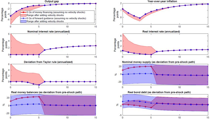
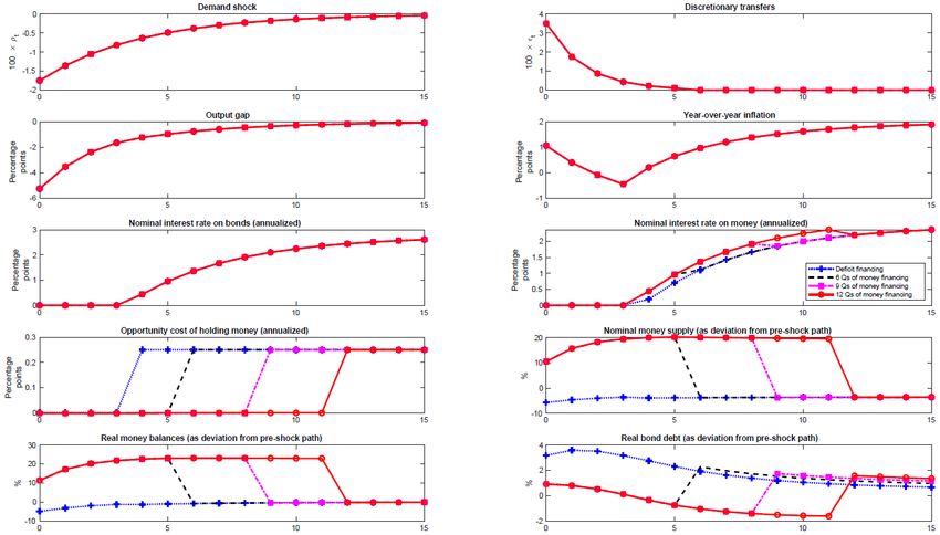
inflation outcomes irrespective of the regime in effect is especially important because inflation,
output and the nominal rate are normally the only variables entering into both ad-hoc and micro-
founded welfare functions. 10
 To summarize the key properties of the two financing regimes before diving into our
simulations, we emphasize the following three take-aways:
(i) Under a money-financing regime, monetary policy is directed toward providing the
 government with a certain amount of seigniorage.
(ii) In this case, the textbook model implies that the nominal policy rate must be set as needed
 to ensure that agents are willing to hold the volumes of money being created, rather than
 being set in line with the central bank’s usual feedback rule, which must (at least temporarily)
 be suspended.
(iii) In the textbook model, differences in output and inflation outcomes across regimes are
 entirely attributable to differences in the implied paths for the nominal interest rate.

3 Money financing versus debt financing in the textbook model
Figure 2 depicts the textbook model’s response to a large demand shock, assuming an illustrative
calibration similar to that in Galí (2019). 11 To isolate the effects of the money-financing versus
debt-financing decision, all simulations assume a common fiscal response to the demand shock,
namely a large discretionary transfer that the government then gradually withdraws over the
course of the next six quarters. Individual simulations differ in the way that these transfers are
financed. More specifically, the blue line corresponds to a standard debt-financing regime, while
the other lines assume money-financing regimes of various durations. For example, the black line
assumes that the central bank commits to money financing for the first year of the simulation.
The pink and red lines extend this commitment to 6 and 8 quarters, respectively. Figure 3 then
repeats for higher-duration commitments to money financing, all the way up to 12 quarters (or
twice the duration of the underlying fiscal program). Unless otherwise noted, all simulations

10
 For example, in the context of the textbook model, it can be shown that a second-order approximation
of the social loss function is given by a weighted sum of the squared deviations of inflation, the output
gap and the nominal rate from appropriately defined target values.
11
 Our only points of departure relative to the calibration in Galí (2019) are that (i) we assume a 2 percent
inflation target; (ii) we re-calibrate households’ subjective discount factor to place the annualized real
neutral rate at the midpoint of the 0.25–1.25 percent range assessed at the time of the Bank’s last neutral
rate update (Carter, Chen and Dorich 2019); (iii) while Galí (2019) assumes a form of strict inflation
targeting tantamount to letting ( , y ) → (∞, 0), we instead set � , y � = (1.5,0.5/4), in line with
Taylor (1993); and (iv) we set the Calvo parameter and inverse Frisch elasticity to 0.8 and 2, respectively,
both somewhat closer to the values assumed in English et al. (2017).

 7

assume perfect foresight, and most variables have been reported in deviations from their pre-
shock paths. The only exceptions are rates of interest and inflation, which we report in levels. 12
 From the figures, we see that the duration of the central bank’s commitment to money
financing is a critical determinant of the benefits that money financing has to offer relative to
debt financing in terms of its ability to boost output and inflation. For example, even though a
four-quarter money-financing regime has the central bank paying for the vast majority of the
underlying fiscal program, it yields no benefits relative to debt financing. In contrast, longer-term
money-financing regimes deliver increasingly powerful levels of stimulus.
 Consistent with the “separability” property emphasized in the previous section, these
outcomes are a direct consequence of the various money-financing regimes’ different
implications for the nominal rate path. For example, the four-quarter money-financing regime
initially involves a year of very low rate settings in order to induce agents to hold the large
volumes of money being created in the early stages of the fiscal program. However, the demand
shock itself is large enough that the ELB would bind even under debt financing for the first year
of the simulation, implying no difference in the resulting rate paths. In contrast, the longer-lived
money-financing regimes imply long intervals during which the central bank must maintain a
relatively more stimulative rate path to ensure that the private sector remains willing to hold the
volumes of money initially created in support of the fiscal program. These more stimulative rate
paths then exert strong upward pressure on output and inflation.
 A key feature of the simulations is that the reinstatement of the Taylor rule after an extended
period of money financing is associated with a sharp increase in the interest rate, along with a
sharp contraction in the nominal money supply. However, the contraction in the nominal money
supply tends to be smaller the longer the initial commitment to money financing is. The dynamic
underlying this pattern is relatively straightforward: longer commitments to money financing
imply greater cumulative stimulus and, therefore, a higher price level at the time that the Taylor
rule is to be re-instated. In turn, the higher price level associates a given level of nominal money
balances with a lower level of real balances. As a result, a smaller contraction in the nominal
money supply is needed to rebalance the money-demand equation at the interest rate implied
by the Taylor rule.
 From Figure 3, we see that this dynamic associates sufficiently long-lived commitments to
money financing with permanent expansions in the nominal money supply of the sort often
emphasized in the literature on helicopter money (e.g., Turner 2015; Bernanke 2016). However,
we stress that the transmission mechanism operating under long-lived regimes is qualitatively no
different from that operating under money-financing regimes of shorter duration—that is, long-
term commitments to money financing do not achieve greater stimulus simply by virtue of their
inducing permanent expansions in the nominal money supply per se, but rather because these

12
 For simplicity, our calibration abstracts from storage costs associated with money holding, so the ELB is
assumed to bind at a nominal rate of zero.

 8

expansions tend to be associated with especially stimulative nominal rate paths in equilibrium.
Moreover, while our results suggest that a permanent suspension of the Taylor rule is not needed
to achieve a large permanent expansion of the nominal money supply, they also suggest that it
may be possible to achieve such expansions only through long-lived departures from the central
bank’s usual feedback rule.
 All that said, the foregoing discussion raises an obvious question: if the benefits of money
financing in terms of its implications for output and inflation are ultimately driven by the
scheme’s implications for the nominal rate path, then could a case be made for using other
unconventional policies, such as forward guidance, to either implicitly or explicitly commit to the
desired path? Before tackling this question in our next section, we re-emphasize the following
two take-aways from figures 2 and 3:
(iv) In the textbook model, a money-financed fiscal expansion will generate more stimulus than
 a debt-financed expansion of the same magnitude only to the extent that money financing
 implies a more stimulative path for nominal interest rates than would be the case under debt
 financing.
(v) The duration of policy-makers’ commitment to money financing is a key determinant of the
 scheme’s overall effectiveness. To achieve high levels of stimulus in the textbook model,
 policy-makers must be prepared to suspend their usual feedback rule for an extended period
 following the withdrawal of the underlying fiscal stimulus.

4 Unstable money demand and other arguments for alternatives to
money financing
 “We didn’t abandon M1, M1 abandoned us.” – Governor Gerald Bouey 13
The status of the nominal rate path as a “sufficient statistic” for predicting output and inflation
outcomes under money financing suggests that it might be possible to achieve similar outcomes
under debt financing. In particular, this would involve (at least temporarily) replacing the Taylor
rule with an alternative monetary policy that implies a nominal rate path close to that obtained
under money financing. While forward guidance is a natural option for engineering such a
replication and will be the main subject of our attention in this section, we note that a variety of
other options for making monetary policy more history-dependent could achieve similar results.
For example, English, Erceg and Lopez-Salido (2017) reach conclusions broadly similar to our own
using an appropriately constructed form of price-level targeting. See Woodford (2012) and
Reichlin, Turner and Woodford (2019) for discussions of alternative approaches involving
nominal GDP targeting.
 We focus on forward guidance because the textbook model has the property that all of the
output and inflation outcomes realized under the money-financing regimes of various durations

13
 See Canada, House of Commons Standing Committee on Finance, Trade and Economic Affairs (1983).

 9

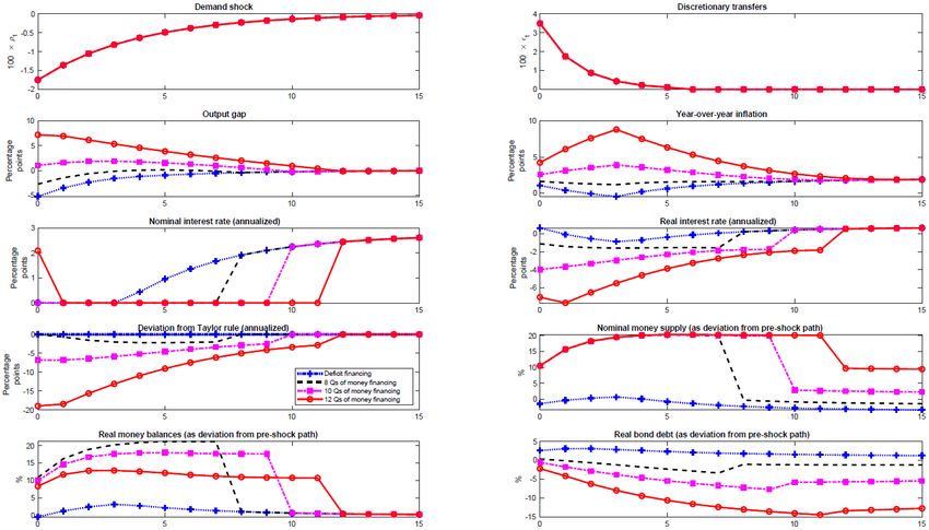
above could be replicated exactly under debt financing if the central bank simply used a period
of forward guidance to commit to following the nominal rate path associated with money
financing. Given our earlier point that inflation, output and the nominal policy rate are the only
variables determining welfare in our model, an approach along these lines would be welfare-
equivalent to money financing from an in-model perspective. However, our view is that a range
of extra-model considerations likely tip the overall balance in favour of forward guidance. These
considerations could also potentially do the same for price-level targeting and other such options
even if these options proved capable of delivering only an approximate replication of the output
and inflation outcomes realized under money financing.
 The first and most obvious of these extra-model considerations is that forward guidance and
other such alternative policies would involve less fiscal-monetary coordination. As a result,
policy-makers would be able to avoid the various political-economic complications that might
arise during extended periods of money financing. These complications include questions that
money financing might raise regarding the (perceived) independence of the central bank and its
longer-run commitment to price stability. There is also a risk that helicopter money might be
perceived to “blur the lines” between fiscal and monetary policy.
 Another key advantage of alternative policies like forward guidance and price-level targeting
is that these are policies under which the central bank directly chooses the level of the nominal
rate. In contrast, money financing involves adjusting the nominal rate as needed to ensure that
the private sector is willing to hold a particular amount of money. For this reason, money-demand
shocks would in the textbook model represent the same threat to money financing as they did
to the failed money-targeting frameworks of the 1970s and 1980s. While those historical
episodes occurred partly as a consequence of specific financial innovations that took place
around the same time, estimated money demand curves remain subject to considerable
volatility. Moreover, to the extent that large demand shocks often originate in the financial
sector, it would not be unusual for them to be accompanied by large swings in the private sector’s
demand for liquidity. As a result, these issues could begin manifesting at precisely the moments
when policy-makers would first begin contemplating money financing.
 A simple way to capture these considerations is by introducing a velocity shock into the
money demand curve 14—i.e.,
 = � − ̂ + if ̂ > ̂ 
 
� � (8)
 ≥ � − ̂ + if ̂ = ̂ .
In Figure 4, we explore this extra shock’s potential implications for the relative merits of forward
guidance versus money financing. More specifically, the red line denotes the economy’s
trajectory under a six-quarter money-financing regime, assuming that no velocity shocks arrive

14
 See Tsuruga and Wake (2019) for a similar case where policy-makers are uncertain of the slope of the
money-demand curve, along with the challenges created by interactions between this source of
uncertainty and fiscal implementation lags.

 10

and that the demand shock and fiscal response both remain in line with our previous simulations.
In contrast, the blue line corresponds to a situation where the central bank follows the same
nominal rate path but does so using six quarters of forward guidance before reinstating its Taylor
rule. For each of these two trajectories, the correspondingly coloured bands denote the ranges
within which outcomes would fall if a velocity shock either coincided with the initial demand
shock or unexpectedly arrived some time later.
 Though our calibration of the persistence and maximum size of velocity shocks is purely
illustrative, the results point to a clear qualitative difference between the two policy regimes in
terms of the variables responsible for absorbing these shocks. In particular, output and inflation
are fully insulated from velocity shocks under forward guidance, but both variables exhibit
substantial volatility under money financing. Intuitively, these differences arise because money-
supply decisions are dictated by fiscal considerations under the money-financing regime,
implying that the interest rate must absorb velocity shocks, which then propagate into output
and inflation via the IS and Phillips curves. In contrast, forward guidance leaves the central bank
free to adjust the money supply as needed to ratify its intended nominal rate path. These
considerations also suggest that it could be difficult to gauge the amount of money financing that
would be needed to achieve a given set of aggregate outcomes.
 All that said, an important drawback associated with forward guidance and other alternative
policies like price-level targeting is that they rely on expectational channels that may break down
if agents are less than fully rational or if monetary policy-makers fail to communicate their plans
clearly and credibly. While these concerns are valid, it is important to note that they also apply
to money financing, since we have already argued that the efficacy of money financing depends
critically on the (perceived) duration of policy-makers’ commitment to monetization and its
implications for the (expected) interest rate path. If anything, the more indirect—and potentially
unstable—nature of the nominal-rate-setting process would presumably make clear, credible
communication even more of a challenge under money financing, relative to forward guidance
and other such alternative policies.
 In the spirit of Poole (1970), another possible objection to forward guidance could be that it
would insulate the economy from velocity shocks at the cost of making it more vulnerable to
aggregate demand shocks. However, this would be an issue only if forward guidance took the
form of an unconditional commitment to a predetermined path for the interest rate. While it is
convenient in the context of our perfect-foresight simulations to model forward guidance in this
simple way, we note that forward guidance would in practice involve degrees of state
contingency that would mitigate Poole’s concerns considerably. For example, the Bank of
Canada’s use of forward guidance in 2009 was explicitly made “conditional on the inflation
outlook” (Bank of Canada 2009a). More exotic variants of state-contingent forward guidance
could include temporary price-level thresholds or targets, as proposed by Mendes and Murchison
(2014) and Bernanke (2017). Making forward guidance state-contingent allows the path of

 11

interest rates to be adjusted in response to demand shocks, thus avoiding the pitfalls of fixed
interest rate paths identified by Poole.
 More generally, this section’s main take-aways can be summarized as follows:
(vi) In the textbook model, the benefits of money financing can be replicated by using other
 policies to achieve the same nominal rate path, most notably including forward guidance.
(vii) Policies like forward guidance have the advantage that they avoid the political-economic
 complications associated with money financing.
(viii)In the textbook model, output and inflation outcomes are vulnerable to money-demand
 shocks under money financing but are fully insulated against these shocks under forward
 guidance and other alternative policies.

5 The role of Ricardian equivalence
Our repeated emphasis on the nominal rate path as the key intermediating variable in the
transmission mechanism for money financing might be somewhat surprising, since much of the
previous literature has emphasized an alternative mechanism having to do with Ricardian
equivalence. More specifically, it is sometimes argued that fiscal expansions should be more
stimulative when financed using a permanent expansion of the money supply rather than debt,
since debt financing may lead to negative wealth effects associated with increases in households’
future tax liabilities (e.g., Turner 2015; Bernanke 2016). In the appendix, we attempt to reconcile
our findings with this Ricardian equivalence-based view and argue that the latter is somewhat
incomplete.
 More specifically, we show that while money financing does not (directly) trigger changes in
households’ future tax liabilities, it still imposes a cost on households in the form of interest
foregone on each dollar of savings allocated to money rather than bonds. Under money financing,
this foregone-interest channel gives rise to wealth effects not dissimilar to those associated with
the tax channel under debt financing. In the special case of representative-agent economies like
the one on which we focus, the two channels prove to be equivalent in the precise sense that
households perceive neither bonds nor money as sources of net wealth after taking both channels
into account. In this sense, both the money- and debt-financing regimes are equally vulnerable
to wealth effects of the sort that the literature has tended to emphasize more heavily in debt-
financing contexts, which is why the results presented above are instead driven by intertemporal-
substitution effects associated with the nominal rate path. In fact, this is a specific example of a
more general point first made by Weil (1991) and more recently emphasized by Harrison and
Thomas (2019), 15 namely that the same conditions giving rise to Ricardian equivalence also tend
to preclude wealth effects associated with changes in the composition of government liabilities.

15
 See also Cohen (1985) and Ireland (2005).

 12

Though we provide further details in the appendix, we briefly note that none of the
arguments presented therein depend on the interest rate on money being exactly zero (or even
strictly less than the interest rate on bonds). As a result, the same reasoning extends to settings
where money takes the form of an interest-bearing asset, including the model to which we turn
our attention in the next two sections.

6 Money versus debt financing in a model with interest-bearing
money
In this section, we relax the textbook assumption that money pays no interest and adapt the
model to recognize that money financing would likely involve the creation of interest-bearing
reserves. To briefly preview our results, we find that the efficacy of money financing diminishes
drastically after taking into account the potential for interest-bearing forms of money. In fact, we
find that money financing of a given fiscal expansion now achieves no additional stimulus
whatsoever, relative to debt financing of an equally sized fiscal expansion.
 To introduce interest on money into the model, we retain most of the structure laid out in
Section 2 but follow Woodford (2003, pp. 101–123 and pp. 295–311) in re-interpreting money as
interest-bearing reserves. The key feature of the resulting model, which can be viewed as a
special case of a more general framework laid out in Harrison and Thomas (2019), is that the
opportunity cost of holding money now depends on the difference between the nominal interest
rate paid on reserves and that paid on other assets. 16 The money demand curve thus reads as

 = � − ( ̂ − ̂ �
 ) if ̂ − ̂ > ∆ı
 
� � (9)
 �
 ≥ � − ∆ı if ̂ − ̂ �
 = ∆ı,

where ̂ denotes the nominal interest rate paid on reserves, expressed as a deviation from its
steady-state value; 17 and ∆ı � denotes a lower bound on the difference ̂ − ̂ at which the
opportunity cost of holding reserves vanishes, making agents content to hold any amount of
balances beyond a satiation level. In Canada, ̂ corresponds to the Bank’s target for the overnight
rate; ̂ 
 corresponds to the lower bound of the operating band for the overnight rate, which is
normally set 25 basis points lower as part of a corridor system.
 In addition, we assume that a small amount of non-interest-bearing currency continues
circulating in the economy, though it accounts for a negligible portion of the overall monetary
base. As a result, all nominal rates in the economy remain subject to an ELB. More generally, our
strategy for introducing interest-bearing reserves into an otherwise standard New Keynesian
setting is meant to capture four key features of the payment system that would likely serve as a

16
 The consolidated government budget constraint must also be expanded to include interest payments
on money. However, as we stress momentarily, the IS and Phillips curves are both unchanged relative to
the textbook model.
17
 Specifically, ̂ 
 ≡ ( − ∗ )/(1 + ∗ ), where denotes the nominal rate paid on reserves, and ∗
denotes the steady state thereof.

 13

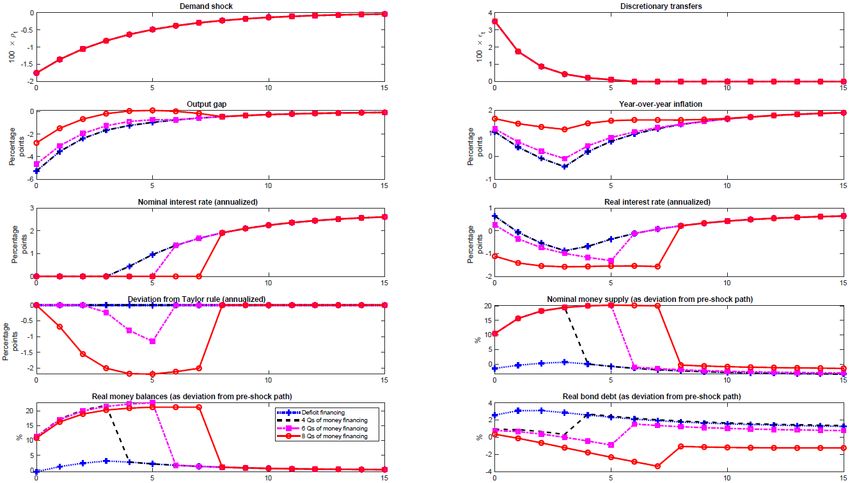
backdrop for the money-financing versus debt-financing decision in a modern economy: (i)
Interest-bearing reserves play a key role in generating liquidity services for the broader economy.
(ii) These reserves also represent the particular form of money on which a money-financing
scheme would likely rely. (Indeed, even if money financing initially relied only on currency
creation, those funds would likely find their way back into the financial system over time, where
banks would face incentives to re-deposit them in interest-bearing form.) At the same time, while
(iii) cash is becoming less and less important over time, (iv) its presence as an outside option still
places a lower bound on nominal returns. Moreover, Piazzesi, Rogers and Schneider (2019) argue
that a money demand curve like equation 9 can generate aggregate results qualitatively in line
with those of a more elaborate framework that models the payment system in greater detail.
 From a policy perspective, the key consequence of introducing an interest rate on money is
that this rate represents an extra degree of freedom in the money demand curve. As a result, the
central bank can now simultaneously set the broad interest rate ̂ in line with its feedback rule
while also engaging in money financing. This would involve adjusting ̂ as needed to keep the
opportunity cost of holding reserves at a level that makes the private sector willing to hold the
volumes of money being created in pursuit of the seigniorage target.
 Figure 5 depicts the model’s behaviour when policy-makers combine money financing with
the pursuit of a Taylor rule, namely by adjusting the interest rate paid on reserves in precisely
the way that we just described. More specifically, the black line in the figure corresponds to a
situation where policy-makers engage in money financing for the first six quarters of the
simulation, after which monetary policy is assumed to return to a more standard “corridor”
configuration under which the central bank maintains a constant 25-basis-point gap between the
interest rate paid on reserves and that paid on other assets. The pink line and red line then repeat
assuming 9- and 12-quarter commitments to money financing, respectively. At the same time,
the blue line denotes a debt-financing benchmark under which the central bank pursues its Taylor
rule while constantly aiming to maintain a corridor configuration.18 (This precludes any form of
money financing to the extent that such a configuration locks in the opportunity cost of holding
reserves.) All simulations assume the same demand shock and fiscal response as in previous
sections, thus allowing us to continue isolating the effects of the money-financing versus debt-
financing decision.
 From the figure, we see that the regimes under consideration all yield identical implications
for output and inflation, though they differ in terms of the composition of government liabilities.
The intuition for this result is that the addition of interest on money has no impact on the IS and

18
 In situations where the central bank cannot simultaneously respect the Taylor rule and maintain a
corridor configuration without driving the interest rate on reserves below the ELB, we assume that policy-
makers prefer a narrower corridor over deviation from the Taylor rule. This is consistent with the Bank’s
experiences in spring 2009, when the target for the overnight rate reached 25 basis points, which was
then assessed to be the ELB, and policy-makers shifted to setting the lower bound of the operating band
equal to the target rate. See Bank of Canada (2009b) for details.

 14

Phillips curves, which still take the forms given above and thus still have the property that the
only policy variable influencing output and inflation outcomes is the path of the broad nominal
interest rate ̂ . Since all of the regimes under consideration have this rate set in line with a
common Taylor rule, the details of the government’s financing plans are irrelevant from the
perspective of output and inflation.
 Given how starkly this result compares with the more nuanced findings emerging from the
textbook model with non-interest-bearing money, it is natural to ask if richer models might leave
some scope for policy-makers to concentrate their money-financing activities in non-interest-
bearing forms of money without fully abandoning the common practice of paying interest on
reserves. Before exploring some “intermediate” policy options of this sort in the next section, we
emphasize the following two take-aways from the model with interest-bearing money:
(ix) If money is interest-bearing, then the model suggests that monetary policy-makers no longer
 need to suspend their usual feedback rule in order to engage in money financing.
(x) In this case, money-supply decisions no longer have any impact on broad nominal interest
 rates, in which case the model predicts that money financing of a given fiscal expansion
 should generate no additional stimulus beyond what could be achieved with debt financing.

7 Tiering and other “intermediate” options
Although it is outside the scope of this paper to fully explore the merits of money financing in
more complicated models where interest- and non-interest-bearing forms of money coexist, the
foregoing discussion suggests a strong case for relying more heavily on the latter when
contemplating money financing in such settings. Of course, when doing so, policy-makers would
have to give careful thought to how they might best contain the incentives that private sector
agents would face to re-deposit non-interest-bearing money in interest-bearing forms.
 A natural candidate on this front would be a tiering system under which a given financial
institution’s reserves are remunerated only up to a threshold beyond which no further interest
is paid. Assuming that this threshold is set to ensure that the marginal dollar is unremunerated,
a tiering system could allow policy-makers to capture many of the benefits associated with
money financing in the textbook model. However, we maintain our above-noted view that these
benefits would be better pursued using forward guidance or other alternative policies. Doing so
would be simpler and significantly more robust to instability in the money-demand curve.
 A potential alternative to tiering might be to use reserve requirements to force financial
institutions to hold a certain amount of non-interest-bearing reserves while still allowing some
degree of remuneration for excess balances. Though superficially similar to tiering, this approach
is in our view unlikely to capture many of the benefits associated with money financing in the
textbook model: since financial institutions’ holdings of non-interest-bearing reserves would be
imposed rather than induced through a market mechanism, changes in the quantity of non-

 15

interest-bearing reserves would likely have little effect on broad nominal rates and thus little
effect on output and inflation.
 To summarize:
(xi) A tiering system would likely make it possible to capture some of the benefits associated
 with money financing in the textbook model without fully abandoning the common practice
 of paying interest on reserves.
(xii) However, in this case, those same benefits could likely be captured more effectively and
 robustly using forward guidance or other such alternative policies.

8 Concluding remarks
Our results suggest that money financing, when studied through the lens of two simple New
Keynesian models, should not be viewed as a way to get more stimulus out of a given fiscal
expansion. More specifically, depending on whether money financing relies on interest-bearing
or non-interest-bearing forms of money, either (i) it would have no stimulative benefits to offer
relative to debt financing, or (ii) all potential benefits could be pursued more effectively and
robustly by combining debt financing with a commitment to a sufficiently accommodative rate
path, implemented using forward guidance or other such alternative policies.
 That said, a potential issue from which our models abstract is that money financing could be
useful in a situation where the government is unable to raise funds in debt markets. Though this
possibility has received some attention in the literature, our view is that a scenario of this sort is
unlikely to arise in advanced economies with their own currencies. Moreover, it seems especially
unlikely that such a situation would arise at a time when the economy is at or near the ELB, which
is precisely when money financing would presumably be contemplated. If anything, ELB episodes
are symptomatic of an excess demand for assets, which should make borrowing relatively easy
for governments able to issue debt in their own currencies.
 Finally, we stress that our analysis is aimed at isolating the effects of the money-financing
versus debt-financing decision by assuming that the government’s spending plans are
independent of the financing regime. As noted earlier, this leaves open a possibility, emphasized
by Bartsch et al. (2019) and several others, that money financing could lead to larger (and
potentially more timely) fiscal expansions relative to those that the government would
implement using debt financing alone. Put differently, while our results do not support using
helicopter money as a way to increase the impact of a given fiscal stimulus, our analysis is silent
on extensive-margin considerations, including the non-economic factors that could influence the
size, form and timing of fiscal programs.

 16