Journal of International Money and Finance
←
→
Page content transcription
If your browser does not render page correctly, please read the page content below

Journal of International Money and Finance xxx (2018) xxx–xxx

                                                        Contents lists available at ScienceDirect

                                Journal of International Money and Finance
                                          journal homepage: www.elsevier.com/locate/jimf

Foreign effects of higher U.S. interest rates q
Matteo Iacoviello ⇑, Gaston Navarro
a
    Federal Reserve Board, Division of International Finance, 20th and C St. NW, Washington D.C. 20551, United States

a r t i c l e           i n f o                         a b s t r a c t

Article history:                                        This paper analyzes the spillovers of higher U.S. interest rates on economic activity in a
Available online xxxx                                   large panel of 50 advanced and emerging economies. We allow the response of GDP in each
                                                        country to vary according to its exchange rate regime, trade openness, and a vulnerability
JEL classification:                                     index that includes current account, foreign reserves, inflation, and external debt. We
F4                                                      document large heterogeneity in the response of advanced and emerging economies to
E5                                                      U.S. interest rate surprises. In response to a U.S. monetary tightening, GDP in foreign econo-
C3
                                                        mies drops about as much as it does in the United States, with a larger decline in emerging
Keywords:                                               economies than in advanced economies. In advanced economies, trade openness with the
U.S. monetary policy                                    United States and the exchange rate regime account for a large portion of the contraction in
Foreign spillovers                                      activity. In emerging economies, the responses do not depend on the exchange rate regime
Local projection                                        or trade openness, but are larger when vulnerability is high.
Macroeconomic transmission                                                                                    Ó 2018 Elsevier Ltd. All rights reserved.
Panel data

1. Introduction

   This paper presents new empirical evidence regarding the cyclical response of foreign economies to U.S. monetary shocks.
We make use of a large dataset exploiting the time-series and cross-sectional variation of foreign economies in their
exchange rate regime, trade openness, and an index of their external vulnerability. Our goal is to gain some empirical sense
of the differential importance of exchange rate channels, trade channels and broad ‘‘financial” channels in response to
changes in U.S. interest rates. Unlike previous studies that have focused on limited time periods, a few countries, or limited
controls, we rely on a comprehensive dataset containing observations on quarterly GDP and time-varying country charac-
teristics for 50 foreign economies for over 50 years. While data quality in international datasets varies systematically across
countries and over time, we believe this is a reasonable price to pay for a dataset that, by exploiting nearly 10,000 observa-
tions, is about two orders of magnitude larger than the typical dataset used to study the domestic effects of U.S. monetary
shocks.
   Fig. 1 shows the federal funds rate from 1965 through 2016. The shaded areas denote periods of rising interest rates. Fig. 2
zooms in on the six tightening episodes before the Global Financial Crisis, showing GDP growth in each episode relative to
what one could have predicted using a simple forecasting model.1 The bars measure average growth surprises from the

 q
    We thank Joshua Herman and Andrew Kane for excellent research assistance. We also thank Jim Hamilton, Andrew Rose, Christopher Erceg, Giovanni
Favara, Zheng Liu, Glenn Rudebusch, and Mark Spiegel for their comments and suggestions. The views expressed are those of the authors and not
necessarily those of the Federal Reserve Board or the Federal Reserve System.
 ⇑ Corresponding author.
    E-mail addresses: matteo.iacoviello@frb.gov (M. Iacoviello), gaston.m.navarro@frb.gov (G. Navarro).
  1
    The forecasting model is, for each country, a univariate autoregressive model for log GDP with four lags and a time trend. To avoid cluttering, some
economies are grouped ex post into regional clusters, with a bar for the average GDP response across them.

https://doi.org/10.1016/j.jimonfin.2018.06.012
0261-5606/Ó 2018 Elsevier Ltd. All rights reserved.

Please cite this article in press as: Iacoviello, M., Navarro, G. Foreign effects of higher U.S. interest rates. J. Int. Money Fin. (2018), https://
doi.org/10.1016/j.jimonfin.2018.06.012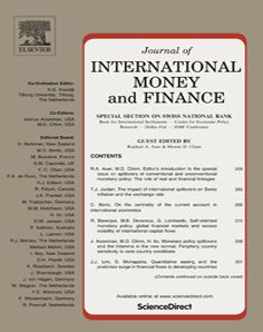
2                                   M. Iacoviello, G. Navarro / Journal of International Money and Finance xxx (2018) xxx–xxx

Fig. 1. The federal funds rate (FFR) from 1965:Q1 through 2016:Q2. Note: The shaded areas denotes periods of interest rate tightenings. A quarter t contains
a tightening if it satisfies any of the following criteria: (1) the FFR does not fall in t and rises by at least 20 and 40 basis points in quarters t  1 and t  2,
respectively; (2) the FFR does not fall by more than 30; 20, and 10 basis points in t; t  1, and t  2, does not fall in t þ 1, and rises by at least 20 and 30 basis
points in t þ 2 and t þ 3; (3) the FFR rises by at least 100 and 200 basis points in t  3 and t  2, and rises by at least 100 basis points in t þ 2.

beginning of each episode until one year after its end. For instance, in panel 1, Mexico’s GDP growth from 1978:Q1
through 1982:Q2 was about 3 percentage points higher, on average, than what one could have predicted using data up to
1977:Q4.2
   The non-uniform pattern of the bars across countries and episodes illustrates how the experience in the aftermath of U.S.
monetary tightenings varies across foreign economies. The high interest rates of the late 1970s–early 1980s eventually led to
lackluster growth in the United States and most foreign economies (panel 1). The tightenings of the 1980s were followed by
weaker growth in many emerging market economies (panels 2 and 3), but the situation was reversed with the higher inter-
est rates of the mid–1990s, which were followed by stronger growth across the board (panel 4). The higher interest rates of
the late 1990s were followed by lower growth among some emerging economies (panel 5). Finally, the most recent tighten-
ing period was followed by an acceleration in growth across all global economies (panel 6). Averaging across episodes,
growth in the United States and advanced economies was slightly higher than forecasted (+0.2 and +0.3%, respectively),
whereas growth in emerging economies was slightly lower (0.4%) in the years after these episodes. Additionally, the dis-
persion across episodes for emerging economies was twice as large as for advanced economies (standard deviation of 2 ver-
sus standard deviation of 0.9). This large dispersion—across and between countries—suggests that not all tightenings are
created equal. The nature of the tightening episode as well as country or region-specific characteristics could account for
their heterogeneous responses.
   This is the perspective adopted here. In the first step, we extract interest rate surprises using quarterly data from 1965
through 2016 to isolate exogenous movements in U.S. interest rates that are unlikely to be correlated with either domestic
or global economic conditions.3 In the second step, we study how the spillovers to foreign economies of interest rate surprises
depend on three factors: (1) the exchange rate regime against the dollar, (2) trade openness with the United States, and (3) an
index of external vulnerability. We use a panel for 50 advanced and emerging economies, and estimate spillovers using a local
projections method (Jorda, 2005). The interest rate spillovers are allowed to differ over time according to these three factors,
and across emerging and advanced economies.

  2
    For each country, the regressions start in 1960:Q1 or later depending on data availability, and are estimated using the full sample. The forecasts are
computed dynamically—using the coefficients estimated for the full sample—starting from the last observation before the monetary tightening. The dynamic
forecasts do not use actual data but exploit the hindsight of knowing the estimated trend growth and AR coefficients for the full sample.
  3
    Most of our focus is on interest rate increases driven by monetary policy shocks. However, Section 6.1 discusses the effect of higher U.S. interest rates due to
improved economic conditions.

Please cite this article in press as: Iacoviello, M., Navarro, G. Foreign effects of higher U.S. interest rates. J. Int. Money Fin. (2018), https://
doi.org/10.1016/j.jimonfin.2018.06.012
M. Iacoviello, G. Navarro / Journal of International Money and Finance xxx (2018) xxx–xxx 3
Fig. 2. Foreign GDP growth relative to forecast after U.S. interest rate increases. Note: Annual GDP growth surprises (actual minus forecast) in each region
relative to ARIMA model in the aftermath of selected U.S. monetary policy tightenings. The bars measure average growth surprises from the beginning of
each episode until one year after its end.
The paper’s main results are:
1. The foreign spillovers of higher U.S. interest rates are large, and on average nearly as large as the U.S. effects. A monetary
policy-induced rise in U.S. rates of 100 basis points reduces GDP in advanced economies and in emerging economies by
0.5% and 0.8%, respectively, after three years. These magnitudes are in the same ballpark as the domestic effects of a U.S.
monetary shock, which reduce U.S. GDP by about 0.7% after two years.
2. In advanced economies, higher U.S. interest rates are transmitted through standard exchange rate and trade channels. In
particular, the responses within advanced economies are larger when a country’s currency is (de facto) pegged to the dol-
lar, or when its trade volume with the United States is high.
3. In emerging economies, exchange rate and trade channels explain little of the differential GDP responses within econo-
mies. Instead, a vulnerability index that we interpret as capturing a country’s financial fragility explains a sizable com-
ponent of differences across economies, with GDP in more vulnerable economies falling much more in response to a
U.S. monetary tightening. This vulnerability index is constructed combining by current account, foreign reserves, infla-
tion, and external debt.
Our estimation methodology exploits both the between- and the within-country variation in a set of observables that are
often viewed as important determinants of the foreign spillovers of U.S. interest rate changes. Several studies that have
recently examined the international effects of U.S. monetary actions using vector autoregressions (VARs) or event studies
have relied on the implicit assumption that many country characteristics that determine such effects are fixed across the
sample.4 Such an assumption is invalidated by the data for virtually all the variables that we consider in our sample, with
all our indicators exhibiting far more variation within than across country borders. For instance, in the 1960s and 1970s, Mexico
had a lower level of trade openness with the United States than South Korea did, but Mexico’s trade exposure grew by a factor of
4
For a list of papers that have examined the foreign effect of higher interest rates, see Kim (2001), Canova (2005), Dedola et al. (2017), Ehrmann and
Fratzscher (2005), Maćkowiak (2007), Di Giovanni and Shambaugh (2008), and Georgiadis (2016). See the Appendix.
Please cite this article in press as: Iacoviello, M., Navarro, G. Foreign effects of higher U.S. interest rates. J. Int. Money Fin. (2018), https://
doi.org/10.1016/j.jimonfin.2018.06.0124 M. Iacoviello, G. Navarro / Journal of International Money and Finance xxx (2018) xxx–xxx
four in the decades since the NAFTA trade agreement, while Korea’s openness remained constant. Similarly, several advanced
economies were effectively pegged to the dollar before the collapse of the Bretton Woods system in 1971, and adopted a floating
exchange rate regime afterwards. More recently, China abandoned its peg to the dollar in 2010, increasing its exchange rate
flexibility. Studies that ignore time-variation in these country characteristics are likely to estimate the effects of interest rate
changes with a large amount of noise.
Section 2 reviews the theoretical underpinnings of the international transmission of interest rate shocks. Section 3
describes the data. Section 4 discusses the methodology and results of the effects of U.S. interest rates shocks. Section 5
extends our methodology to look at state-dependent effects of interest rate shocks. Section 6 contains robustness analysis.
Section 7 contains a historical quantification of the effect of U.S. monetary shocks on foreign economies. Section 8 concludes.
2. Channels of international interest rate transmission
2.1. The channels
Models of international interest rate transmission typically emphasize exchange rate channels, trade channels, and finan-
cial channels as key determinants of the response of foreign economies to changes in interest rates in another country.5 The
first two channels are a staple of virtually all general equilibrium, intertemporal models of macroeconomic policy transmission
that merge Keynesian pricing assumptions and international market segmentation building on the Mundell-Fleming-Dornbusch
framework.6 Financial channels have been emphasized in recent work that has studied the international implications of various
types of credit market frictions.7
The exchange rate channel is predicated on the idea of demand substitution between domestic and foreign-produced
goods, and implies that higher interest rates in the United States may lead to an expansion of activity abroad. Consider,
for instance, an increase in interest rates in the United States. Via the uncovered interest parity condition, higher U.S. interest
rates lead to an appreciation of the dollar. In turn, the stronger dollar moves the composition of world demand away from U.
S. goods and towards goods produced in other countries. With flexible exchange rates, GDP in foreign economies should rise,
boosted by cheaper exports. By contrast, a country that pegs its exchange rate to the dollar should experience an appreci-
ation that lowers its GDP.
The trade channel rests on the idea that higher U.S. interest rates reduce incomes and expenditures in the United States,
thus leading to lower U.S. demand for both domestically produced and imported goods, and reducing activity and GDP
abroad.8 Overall, the strength of this channel should depend on the share of exports and imports in economic activity (the trade
exposure), especially with the United States.
Financial channels capture the idea that higher U.S. interest rates can spillover to the price of various financial assets and
liabilities held abroad, thus affecting activity in foreign countries even after controlling for exchange rate and trade channels.
For instance, when domestic agents are credit constrained and hold dollar denominated debt, an increase in U.S. interest
rates may lead to a deterioration of domestic balance sheets in the presence of flexible exchange rates.9 A common theme
behind the financial channels is that frictions that prevent intertemporal smoothing through foreign borrowing and lending
may magnify the impact of foreign shocks for economies that are integrated with the world markets. These frictions can be
exacerbated when the fundamentals of a country are weak. For instance, high inflation may create political instability and con-
strain domestic monetary and fiscal responses to adverse shocks. Similarly, a large current account deficit or low foreign
reserves may put a country at risk of facing financial pressure from foreign lenders.
Recent work has also highlighted the importance of global factors that can propagate changes in one country’s monetary
conditions to the rest of the world, especially when capital markets are highly integrated. Rey (2015) and Miranda-Agrippino
and Rey (2017) show that changes in interest rates in ‘‘core” countries can trigger a global financial cycle that, regardless of
the exchange rate regime, may generate positive global spillovers. Bruno and Shin (2015) find evidence of monetary policy
spillovers on cross-border capital flows. This work highlights channels that seem to operate independently of, and above, the
traditional exchange rate and trade channels.
2.2. Disentangling the channels
Is it possible to tell these channels apart? Without loss of generality, consider an increase in U.S. interest rates driven by
an exogenous monetary shock.
5
We borrow this classification from Ammer et al. (2016). Blanchard et al. (2010) discuss a similar set of channels in accounting for the impact of the Global
Financial Crisis on emerging economies. See also Kim (2001).
6
See for instance the work of Obstfeld and Rogoff (1995) for a modern, micro-founded exposition of this framework.
7
See for instance Aghion et al. (2004) and Gertler et al. (2007).
8
See Erceg et al. (2005) for a two-country DSGE model where demand shocks in one country yield positive output spillovers to another country via the trade
balance channel.
9
These ‘‘financial accelerator” effects may work even with fixed exchange rates. When a country pegs its exchange rate, the rise in domestic nominal interest
rate which is required to maintain the peg may lead to a significant increase in the country’s real borrowing costs. In turn, the rise in borrowing costs may
induce a contraction in output which is further magnified by asset price channels operating through the financial accelerator.
Please cite this article in press as: Iacoviello, M., Navarro, G. Foreign effects of higher U.S. interest rates. J. Int. Money Fin. (2018), https://
doi.org/10.1016/j.jimonfin.2018.06.012M. Iacoviello, G. Navarro / Journal of International Money and Finance xxx (2018) xxx–xxx 5
If the exchange rate channel is important, the exchange rate regime should explain a substantial portion of the cross-
country variation in GDP response following an increase in U.S. interest rates. In particular, the traditional version of this
channel predicts that a country that pegs its exchange rate to the dollar should experience a larger negative GDP response.
If trade channels are important, trade intensity with the United States should matter for the cross-country GDP response
to higher U.S. interest rates, even after controlling for the exchange rate response. In particular, this channel predicts that
higher levels of trade with the United States will lead to a larger GDP contraction in response to an increase in U.S. interest
rates, as the decrease in U.S. demand spills over to the exports of the largest U.S. trading partners.
All other transmission mechanisms fall under the category of financial channels. By financial channels, we mean
mechanisms that stem from the presence of various forms of market imperfections and that operate above and
beyond the standard Mundell-Fleming-Dornbusch model. Suppose that we have already controlled for exchange rate
regime and trade openness with the United States in assessing the foreign GDP response to U.S. interest rate shocks.
We conjecture that, if additional financial variables can explain residual differences in how countries respond to U.S.
interest rate changes, these additional variables are likely to capture the role of financial channels in international
business cycles.
To what extent can we measure the strength of financial channels in the international transmission of monetary
policy? Our strategy is to construct a summary indicator of variables that have a high probability of signaling the
weakness in the economic fundamentals of a country. For practical purposes, these variables must be readily available
and be somewhat consistently defined across countries and over time. In our analysis, we focus on four variables: a
country’s current account deficit, foreign reserves, inflation, and external debt. We combine these four variables in a
summary indicator which combines them using equal weights, and we label this summary indicator the vulnerability
index.
The above classification is obviously a simplification, and we illustrate potential pitfalls with one example. It is possible
that the exchange rate channel matters but not through the standard dollar anchoring classification that we use. For
instance, the exchange rate channel might be captured by trade invoicing, as discussed by Gopinath (2015).10 U.S. monetary
policy might matter because exports and imports are priced in U.S. dollars regardless of the exchange rate regime. Channels of
this kind—or broadly-based confidence channels based on the outsize role of U.S. monetary policy—could also capture residual
differences in the effects of higher U.S. interest rates, but we do not control for them in our analysis.
3. The data
This Section describes the data used in our paper. Additional details on the sources are provided in the Appendix.
3.1. Data on GDP
Our main focus is on the effects of changes in U.S. interest rates on foreign real GDP. To this end, we put together a novel
dataset containing quarterly GDP data for 50 foreign economies (25 advanced and 25 emerging) plus the United States. The
coverage, which varies across countries, spans from as early as 1965:Q1 to as late as 2016:Q2.
Our benchmark analysis uses GDP data for the countries listed in Table 1. For some countries, we extend backward the
original, publicly available quarterly GDP series using annual GDP data that are available from the World Bank’s World
Development Indicators. To convert the annual data into a quarterly frequency, we use Denton’s proportional interpolation
method (Chen, 2007). For emerging economies, the ‘‘indicator series” used for interpolation is the purchasing power parity
(PPP) weighted GDP of the emerging economies for which quarterly GDP data are available. We adopt a similar procedure for
advanced economies, where the interpolation method uses PPP-weighted GDP of the other advanced economies (excluding
the United States).
3.2. Control variables: the exchange rate regime, trade openness, and vulnerability index
Our analysis also focuses on how specific variables across countries affect the spillovers from interest rate changes to GDP
outcomes. To this end, we compile data on the exchange rate regime against the dollar, trade openness with the United
States, and other variables for all the countries in the dataset. We use these data to construct indexes of (1) exchange rate
exposure, (2) trade exposure, and (3) external vulnerability.
1. For the exchange rate regime, we draw on the narrative analysis of Ilzetzki et al. (2017) and our own analysis of the lit-
erature to construct an index ranging from 0 to 1 for each country and period. We classify a country as 0 if it maintains a
flexible exchange rate against the U.S. dollar, 1/2 if it maintains an exchange rate band, and 1 if it pegs against the dollar.
In sum, the index takes on higher values the ‘‘more” a country pegs its exchange rate to the dollar.
2. For each country, we measure its trade openness with the United States by taking the sum of exports to, and imports
from, the United States, divided by GDP.
10
Long-span information on trade invoicing is scant. Gopinath (2015)’s index of trade invoicing starts in 1999.
Please cite this article in press as: Iacoviello, M., Navarro, G. Foreign effects of higher U.S. interest rates. J. Int. Money Fin. (2018), https://
doi.org/10.1016/j.jimonfin.2018.06.0126 M. Iacoviello, G. Navarro / Journal of International Money and Finance xxx (2018) xxx–xxx
Table 1
Data availability.
Country GDP Dollar Peg Trade U.S. Curr.Acct. Reserves Inflation Ext.Debt
First Firstq Last First Last First Last First Last First Last First Last First Last
Argentina 1965 1993 2016 1965 2016 1971 2016 1970 2016 1970 2016 1965 2016 1970 2016
Australia 1965 1965 2016 1965 2016 1965 2016 1970 2016 1970 2016 1965 2016 1970 2016
Austria 1965 1970 2016 1965 2016 1965 2016 1970 2016 1970 2016 1965 2016 1970 2016
Belgium 1965 1970 2016 1965 2016 1965 2016 1994 2016 1970 2016 1965 2016 1970 2016
Botswana 1965 1994 2016 1965 2016 1974 2016 1974 2016 1975 2016 1965 2016 1975 2016
Brazil 1965 1990 2016 1965 2016 1982 2016 1970 2016 1970 2016 1965 2016 1970 2016
Canada 1965 1965 2016 1965 2016 1965 2016 1970 2016 1970 2016 1965 2016 1970 2016
Chile 1965 1996 2016 1965 2016 1965 2016 1970 2016 1970 2016 1965 2016 1970 2016
China 1965 1992 2016 1965 2016 1972 2016 1981 2016 1976 2016 1965 2016 1980 2016
Colombia 1965 2000 2016 1965 2016 1965 2016 1970 2016 1970 2016 1965 2016 1970 2016
Czech Republic 1990 1996 2016 1965 2016 1993 2016 1992 2016 1992 2016 1971 2016 1992 2016
Denmark 1965 1966 2016 1965 2016 1965 2016 1970 2016 1970 2016 1967 2016 1970 2016
Ecuador 1965 1990 2016 1965 2016 1965 2016 1970 2016 1970 2016 1965 2016 1970 2016
El Salvador 1965 1990 2016 1965 2016 1965 2016 1970 2016 1970 2016 1965 2016 1970 2016
Finland 1965 1970 2016 1965 2016 1965 2016 1970 2016 1970 2016 1965 2016 1970 2016
France 1965 1965 2016 1965 2016 1965 2016 1970 2016 1970 2016 1965 2016 1970 2016
Germany 1970 1970 2016 1965 2016 1970 2016 1970 2016 1970 2016 1965 2016 1970 2016
Greece 1965 1970 2016 1965 2016 1965 2016 1970 2016 1970 2016 1965 2016 1970 2016
Hong Kong 1965 1990 2016 1965 2016 1965 2016 1997 2016 1970 2016 1965 2016 1978 2016
Hungary 1991 1995 2016 1965 2016 1991 2016 1991 2016 1991 2016 1967 2016 1991 2016
Iceland 1965 1997 2016 1965 2016 1965 2016 1970 2016 1970 2016 1965 2016 1970 2016
India 1965 1996 2016 1965 2016 1965 2016 1970 2016 1970 2016 1965 2016 1970 2016
Indonesia 1965 1984 2016 1965 2016 1967 2016 1970 2016 1970 2016 1965 2016 1970 2016
Ireland 1965 1965 2016 1965 2016 1965 2016 1970 2016 1970 2016 1965 2016 1970 2016
Israel 1965 1995 2016 1965 2016 1965 2016 1970 2016 1970 2016 1965 2016 1970 2016
Italy 1965 1970 2016 1965 2016 1965 2016 1970 2016 1970 2016 1965 2016 1970 2016
Japan 1965 1965 2016 1965 2016 1965 2016 1970 2016 1970 2016 1965 2016 1970 2016
Jordan 1975 1992 2016 1965 2016 1975 2016 1975 2016 1975 2016 1970 2016 1975 2016
Korea 1965 1965 2016 1965 2016 1965 2016 1970 2016 1970 2016 1965 2016 1970 2016
Luxembourg 1965 1965 2016 1965 2016 1997 2016 1970 2016 1983 2016 1965 2016 1989 2016
Malaysia 1965 1991 2016 1965 2016 1966 2016 1970 2016 1970 2016 1965 2016 1970 2016
Mexico 1965 1980 2016 1965 2016 1965 2016 1970 2016 1970 2016 1965 2016 1970 2016
Netherlands 1965 1965 2016 1965 2016 1965 2016 1970 2016 1970 2016 1965 2016 1970 2016
New Zealand 1965 1965 2016 1965 2016 1965 2016 1977 2016 1977 2016 1965 2016 1977 2016
Norway 1965 1970 2016 1965 2016 1965 2016 1970 2016 1970 2016 1965 2016 1970 2016
Peru 1965 1980 2016 1965 2016 1965 2016 1970 2016 1970 2016 1965 2016 1970 2016
Philippines 1965 1981 2016 1965 2016 1965 2016 1970 2016 1970 2016 1965 2016 1970 2016
Poland 1990 1995 2016 1965 2016 1990 2016 1990 2016 1990 2016 1971 2016 1990 2016
Portugal 1965 1965 2016 1965 2016 1965 2016 1971 2016 1970 2016 1965 2016 1971 2016
Singapore 1965 1975 2016 1965 2016 1965 2016 1970 2016 1970 2016 1965 2016 1970 2016
South Africa 1965 1965 2016 1965 2016 1965 2016 1970 2016 1970 2016 1965 2016 1970 2016
Spain 1965 1970 2016 1965 2016 1965 2016 1970 2016 1970 2016 1965 2016 1970 2016
Sweden 1965 1965 2016 1965 2016 1965 2016 1970 2016 1970 2016 1965 2016 1970 2016
Switzerland 1965 1965 2016 1965 2016 1965 2016 1980 2016 1980 2016 1965 2016 1980 2016
Taiwan 1965 1965 2016 1965 2016 1965 2016 1970 2016 1970 2016 1965 2016 1976 2016
Thailand 1965 1993 2016 1965 2016 1965 2016 1970 2016 1970 2016 1965 2016 1970 2016
Turkey 1965 1987 2016 1965 2016 1965 2016 1970 2016 1970 2016 1965 2016 1970 2016
United Kingdom 1965 1965 2016 1965 2016 1965 2016 1970 2016 1970 2016 1965 2016 1970 2016
United States 1965 1965 2016 1965 2016 1970 2016 1970 2016 1965 2016 1970 2016
Venezuela 1965 1997 2015 1965 2016 1965 2016 1970 2016 1970 2016 1965 2016 1970 2016
Note: Data coverage for each of the variables included in the panel. The GDP data span the period between columns ‘‘first” and ‘‘last.” For some countries,
we extend backward the original quarterly GDP series—available starting in the year listed in column ‘‘firstq”—using annual GDP data that are available
from the World Bank’s World Development Indicators. To convert the annual data into a quarterly frequency, we use Denton’s proportional interpolation
method (Chen, 2007).
3. Our external vulnerability index is an equally-weighted average of four indicators that we use to measure the financial
‘‘health” of a country11:
(a) Inflation, measured in each country by the year-on-year change in the headline consumer price index;
(b) Current account deficit, expressed as a share of GDP;
(c) External debt less foreign exchange reserves, expressed as a share of GDP;
11
Some of these indicators are not available early in the sample, as shown in Table 1. To avoid dropping observations relative to our benchmark analysis, we
fill in the missing observations using backward extrapolation. For instance, we assume that the current account position of a country in 1965–1969 is equal to
its 1970 value. Repeating this analysis without filled-in observations yields nearly identical results to those reported in the paper.
Please cite this article in press as: Iacoviello, M., Navarro, G. Foreign effects of higher U.S. interest rates. J. Int. Money Fin. (2018), https://
doi.org/10.1016/j.jimonfin.2018.06.012M. Iacoviello, G. Navarro / Journal of International Money and Finance xxx (2018) xxx–xxx 7
(d) Foreign exchange reserves, expressed as a share of GDP.
4. Average spillovers of higher U.S. interest rates
In this section, we estimate the foreign and domestic spillovers of higher U.S. interest rates. We consider higher rates as a
scenario in which the policy rate is higher than what could have been predicted using an estimated feedback rule.12 In this
section, we estimate the average international spillover of higher rates, while Section 5 discusses how this spillovers may
depend on the economy’s exposure to exchange rate, trade, and financial vulnerability channels.
4.1. Identification of U.S. monetary shocks
We identify U.S. monetary shocks by regressing the federal funds rate on a set of controls, and use the residuals as the
identified shocks. In particular, we estimate shocks ut as the residual in following regression:
rt ¼ h0 þ h1 Z t þ ut ð1Þ
where r t is the federal funds rate. The set of controls Z t includes contemporaneous and lagged values of inflation, log U.S.
GDP, corporate spreads, log foreign GDP, as well as lagged values of the federal funds rate and a quadratic time trend.13
Because we include current macroeconomic variables as controls, our shock identification is analogous to a Cholesky identifi-
cation in a VAR that orders the federal funds rate last, as done by Christiano et al. (2005) and others.14 We use quarterly data
from 1965:Q1 to 2016:Q2, and replace the federal funds rate with the Wu-Xia shadow rate from 2009 to 2015 to account for the
zero lower bound and for the stimulus to the economy provided by the unconventional monetary policy actions that followed
the Great Recession.15
Fig. 3 plots the identified monetary shocks. The largest contractionary shocks are in the early 1980s during the Volcker
tightening period, and in 2008 at the onset of the zero-lower-bound era. In recent years, the identified shocks point to a
tightening of policy in 2013, around the period of the taper tantrum, as well as to an easing in 2014 and 2015.
4.2. Estimation of the foreign effects
With the identified monetary shocks at hand, we compute the dynamic responses of foreign and U.S. GDP using the local
projection method developed by Jorda (2005). This method allows us to compute the response of variables to shocks at dif-
ferent horizons without imposing many structural restrictions. This flexibility can be easily extended to estimate state-
dependent responses, which eases comparison with the findings of the next section, where we compute responses as a func-
tion of the economy’s exposure to interest rate shocks.16
For computing the response of U.S. GDP, we estimate the following equation:
ytþh ¼ ah þ bh ut þ Ah Z t þ tþh for h ¼ 0; 1; 2; . . . ; H ð2Þ
where ytþh is U.S. GDP in quarter t þ h; ut is the monetary shock, and Z t is a set of controls. A plot of fbh g is the dynamic
response of U.S. output to an innovation in ut . We also estimate Eq. (2) using the federal funds rate as ytþh to compute its
response to the identified shock. In both cases, the set of controls Z t includes four lags of yt and a quadratic time trend.
We take advantage of the panel dimension when computing the foreign GDP response to the monetary shock. In partic-
ular, we estimate a version of (2) as follows:
yi;tþh ¼ ai;h þ bh ut þ Ah;i Z i;t þ i;tþh for h ¼ 0; 1; 2; . . . ; H ð3Þ
where yi;tþh is the GDP of country i in quarter t þ h, and ai;h is a country-specific fixed effect. Notice that we project all
countries on the same shock ut . Accordingly, fbh g measures the average response of output across countries to an innovation
in ut . Controls Z i;t include four lags of country i’s GDP, as well as a linear and a quadratic trend.17
We are interested in documenting how responses to higher U.S. rates may differ across advanced and emerging econo-
mies. To this end, we estimate Eq. (4) separately for advanced and emerging economies.
12
We also analyzed the effects of an alternative scenario in which monetary policy endogenously responds to improved domestic conditions. The results of
this alternative scenario are discussed in Section 6.
13
We use four lags for all variables. Inflation is measured as the four-quarter change in the GDP deflator. Corporate spreads correspond to the difference
between the Moody’s seasoned Baa corporate bond yield and the 10-Year Treasury note yield at constant maturity. We construct an index of foreign GDP by
cumulating the average of quarter-on-quarter GDP growth for the countries in the sample. Each quarter, the weights are based on each country’s GDP in
constant US dollars from the World Bank World Development Indicators (if data for a country are not available, its weight is set at zero, and the weights of other
countries are changed accordingly).
14
Our results below are robust to using the monetary shocks measure constructed by Romer and Romer (2004). See Section 6.
15
See Wu and Xia (2016) for details.
16
See, for instance, Auerbach and Gorodnichenko (2013) for a recent example of state-dependent multipliers estimation using Jorda (2005)’s local projections
method.
17
We let the coefficients on the controls Z i;t be country-specific. Assuming common coefficients across countries makes foreign responses to U.S. monetary
shocks marginally larger than in the specification presented here.
Please cite this article in press as: Iacoviello, M., Navarro, G. Foreign effects of higher U.S. interest rates. J. Int. Money Fin. (2018), https://
doi.org/10.1016/j.jimonfin.2018.06.0128 M. Iacoviello, G. Navarro / Journal of International Money and Finance xxx (2018) xxx–xxx
Fig. 3. Identified monetary shocks. Note: The shocks are calculated as the residuals of a regression of the federal funds rate on contemporaneous and lagged
values of inflation, log U.S. GDP, corporate spreads, log foreign GDP, as well as lagged values of the federal funds rate and a quadratic time trend.
4.3. Results: U.S. monetary policy matters
Fig. 4 shows the response of U.S. GDP, the federal funds rate, and foreign GDP to a monetary shock. The shaded areas
denote 68% confidence intervals and are based on robust standard errors that account for serial correlation (in the case of
the U.S. responses) and for clusters by time and country (in the case of the foreign responses).18 A shock that increases
the federal funds rate by 1 percentage point induces a lasting decline in U.S. GDP, which contracts output by 0:7% after two years
and recovers thereafter. The magnitude and duration of the U.S. output response to a monetary shock is largely in line with pre-
vious findings in the literature (Ramey, 2016).
The dynamic response of GDP in advanced foreign economies follows a similar profile to the U.S. one, but is smaller and
more delayed, with GDP dropping by about 0:5% three years after the shock. The GDP response of emerging economies is as
delayed as that of the advanced economies, but eventually as large as the one in the United States, with GDP falling 0:7% four
years after the shock. All told, the results highlight how emerging economies are more exposed than advanced economies to
higher U.S. interest rates.
5. Foreign effect of higher U.S. interest rates: disentangling the channels of transmission
We turn now to estimating how a country’s dynamic response to a monetary shock depends on exchange rate, trade, and
financial channels.
5.1. Methodology
Consider a set of variables v 2 V that measure the exposure of an economy to higher U.S. interest rates, and let higher
values of v represent higher exposure. To estimate how exposure affects the economy’s response to a monetary shock, we
extend the specification in Eq. (3) so that the identified shock interacts with the measures of exposure. In particular, we esti-
mate the following equation:
X v ?
yi;tþh ¼ ai;h þ bh ut þ bh evi;t1 ut þ Ah;i Z i;t þ i;tþh for h ¼ 0; 1; 2; . . . ; H; ð4Þ
v 2V
?
where evi;t is the exposure index for variable v. The interaction term evi;t1 ut is constructed so that bh captures the response
to a shock when the exposure measures are at their median values, and bvh represents the marginal response to the shock
when exposure evi;t1 is high.
?
We construct the interaction term evi;t1 ut in five steps. First, we standardize each exposure variable v i;t by subtracting
its mean and dividing by its variance. 19
Second, we construct a logistic transformation of the standardized variable (v si;t ) as
18
We calculate the confidence bands using the Driscoll and Kraay (1998) standard errors that already allow arbitrary correlations of the error term across
countries and time.
19
The standardization is a simple device to put all variables on equal footing, and follows the lead of many, including Auerbach and Gorodnichenko (2013)
and Herrera and Garcia (1999).
Please cite this article in press as: Iacoviello, M., Navarro, G. Foreign effects of higher U.S. interest rates. J. Int. Money Fin. (2018), https://
doi.org/10.1016/j.jimonfin.2018.06.012M. Iacoviello, G. Navarro / Journal of International Money and Finance xxx (2018) xxx–xxx 9
Fig. 4. Responses to a monetary shock. Note: Impulse response to a U.S. monetary shock in the benchmark specification. AFE denotes advanced foreign
economies, EME denotes emerging market economies. GDP is in percent deviation from baseline. Federal funds rate is in percentage points. The shaded
areas deNote 68% confidence intervals.
n o
exp vs ‘v ‘v
‘vi;t ¼ ni;t o. Third, we re-center ‘vi;t in terms of the distance between its 50th and its 95th percentile: evi;t ¼ ‘vi;t ‘50 v
v , where ‘p
1þexp v si;t 95 50
corresponds to the pth percentile of ‘vi;t . Fourth, we construct the interaction term evi;t1 urt . Finally, we orthogonalize
evi;t1 urt using a recursive procedure. For the first exposure variable v 1 , we regress evi;t1 1
urt on ut ; Z i;t and obtain the residual
? ? ?
evi;t1
1
urt . For the second variable v 2 , we regress evi;t1
2
urt on ut ; Z i;t ; evi;t1
1
urt and obtain the residual evi;t1
2
urt . We pro-
ceed in a similar vein with the other exposure measures.20
The standardization step makes all the exposure variables comparable. The logistic transformation maps variables to the
unit interval which allows us to consider them in distributional/probabilistic terms.21 The re-centering step allows us to inter-
pret the coefficients as deviations from median levels of exposure. In particular, bh is the response to the shock when all expo-
sure indexes are at their median value, and bh þ bvh is the response when the exposure index evi;t is at the 95th percentile of its
distribution.
The orthogonalization step eases interpretation and comparison with Section 4.3. In particular, because all the interaction
terms are orthogonal to the shock urt , the bh estimated in Eq. (4) is identical to the one from Eq. (3). Thus, we keep considering
fbh g as the average response to the shock. Furthermore, because each additional exposure measure is orthogonal to the pre-
vious ones, we can interpret bvh as the marginal effect of variable v on the pass-through of the monetary shock to foreign GDP
when v moves from the 50th to the 95th percentile of its distribution.
5.2. Exposure variables
In practice, we consider three measures of exposure that capture the three channels discussed in Section 2.
1. Exchange Rate Channel: We construct a variable measuring the degree to which a country’s currency is pegged to the
dollar. The variable equals 0 when a country has a flexible exchange rate against the dollar, 0:5 if the country pegs against
the dollar within a somewhat large band (±5%), and 1 if the country is closely pegged to the dollar (including a ±2% band).
We consider countries with a higher degree of anchoring to the dollar as more exposed to U.S. monetary shocks, as higher
U.S. rates would induce an appreciation of the dollar—and thus, the domestic currency—which depresses GDP by making
imports cheaper and exports more expensive. The median observation in our sample for advanced economies is a flexible
exchange regime, which applies to 80% of the country-quarter observations. Instead, the median for emerging economies
is a system with a close anchor to the dollar, which applies to 55% of the observations.22
2. Trade Channel: We measure the amount of trade with the United States (exports plus imports) as a fraction of the coun-
try’s GDP. Note that the median amount of trade with the United States is about 3.5% of GDP for advanced economies
(such as the United Kingdom in the 2000s), and around 10% of GDP for emerging economies (such as Chile in the 2000s).
? ? ?
20
More generally: for the nth exposure variable v n , we regress evi;t1
n
urt on ut ; Z i;t ; evi;t1
1
urt ; evi;t1
2
urt ; . . . ; evi;t1
n1
urt and obtain the residual
?
evi;t1
n
urt . This procedure is known as regression by successive (Gram-Schmidt) orthogonalization. See for instance Balli and Sørensen (2013) for an
application to regressions with interaction effects.
21
The logistic transformation is a simple manner to estimate the state-dependent effect of shocks that has been extensively used in recent work. See
Auerbach and Gorodnichenko (2017) and Ramey (2016).
22
Ilzetzki et al. (2017) also note that, by their classification, the U.S. dollar scores by a wide margin as the world’s dominant anchor currency.
Please cite this article in press as: Iacoviello, M., Navarro, G. Foreign effects of higher U.S. interest rates. J. Int. Money Fin. (2018), https://
doi.org/10.1016/j.jimonfin.2018.06.01210 M. Iacoviello, G. Navarro / Journal of International Money and Finance xxx (2018) xxx–xxx
Table 2
Summary statistics for the exposure measures.
Advanced economies Emerging economies
Exposure variables 5% Median 95% 5% Median 95%
Exchange rate regime versus dollar 0 0 1 0 0.85 1
Trade openness with the U.S., % 1.3 3.5 17.8 1.9 9.8 34.4
Inflation rate 0.6 3.4 18.3 0.6 7.5 88.2
Current account deficit, % of GDP 6.9 0.3 4.9 8.5 0.5 4.4
Foreign reserves, % of GDP 0.4 2.3 16.5 0.4 5.1 66.1
External debt minus reserves, % of GDP 2.1 29.9 361.6 31.4 11.4 75.0
Note: All variables computed as 12-quarters moving averages. The exchange rate regime ranges from zero (flexible exchange rate vis-à-vis the dollar) to one
(fixed regime). Trade openness is the sum of nominal merchandise imports and nominal merchandise exports, divided by nominal GDP. The vulnerability
index is an equally-weighted average of a logistic transformation of a country’s inflation, current account deficit, foreign reserves (with a negative sign), and
external debt.
3. Financial Channel: We construct a vulnerability index as an equally-weighted average of the following four variables: cur-
rent account deficit, foreign reserves (entering with a negative sign), inflation, and external debt.23
A large current account deficit may limit the willingness of foreign lenders to extend credit, or may even trigger sharp capital
outflows, especially in the presence of high interest rates abroad. Additionally, evidence from Claessens et al. (2010) indi-
cates that large current account deficits raise the incidence and severity of a crisis.
Both credit risk agencies and international organizations frequently consider foreign reserves and external debt in assessing
the external vulnerability of a country. See for instance Santacreu (2015). Additionally, there is evidence that both variables
are important in capturing the sensitivity of an economy to adverse shocks. For instance, Frankel and Saravelos (2012) sug-
gest that central bank reserves are one of the leading indicators in explaining crisis incidence across different countries. Lane
and Milesi-Ferretti (2017) indicate that excessive reliance on debt finance may increase a country’s actual and perceived vul-
nerability.
Although not a direct measure of financial channels, we also include inflation—measured by the annual change in
the consumer price index—in our vulnerability index. High inflation may indicate structural problems in a govern-
ment’s finances, or could generate political instability which in turn acts as an amplifier of the effects of higher
U.S. interest rate. High inflation may also increase the sensitivity of a country’s borrowing costs to changing
interest rates. For instance, Cantor and Packer (1996) find that inflation is a significant determinant of sovereign
ratings.
For each variable, we take a three-year moving average and truncate observations on both sides at a 5% threshold in order
to remove outliers and to guard against extreme measurement error—to us, it seems immaterial whether a country has a 100
or a 1000% inflation rate. The three exposure measures are constructed separately for advanced and emerging economies.
Table 2 presents the summary statistics for the exposure variables in our analysis. The vulnerability index is constructed
so that it takes on high values when foreign reserves are low, and when inflation, external debt, and the current account
deficit are high.
To give a visual impression of the evolution of these indicators, Fig. 5 plots the recent evolution of the three exposure
measures for a selected sample of countries.24 The figure showcases the evolution of our exposure measure over time and
across countries, which allows us to measure the heterogeneous effects of U.S. interest rates. The top left panel shows how
Canada, Japan, and the United Kingdom have at some point in the past abandoned their peg to the dollar.25 Canada, for instance,
was closely pegged to the dollar until 2002, kept a managed floating regime between 2002 and 2010, and moved to a floating
exchange regime thereafter.
The orthogonalization procedure merits some discussion. This procedure is a convenient method to illustrate the mar-
ginal effect of each exposure variable after controlling for the others. However, it also implies that the particular ordering
of the exposure measures matters. We choose the ordering in a way that conforms closely to the historical evolution of
the channels. The exchange rate channel is perhaps the most intuitive and natural, and we order it first. The trade channel
matters over and above the exchange rate channel, and we order it second. Finally, the financial channel is a residual channel
that captures forces that operate beyond the standard channels, and we order it last. That said, there is little correlation in
the data across our exposure measures. Therefore, we experimented with different orderings and found very similar quan-
titative results.
23
As an alternative to an equally-weighted average, we also considered the first principal component. The results were qualitatively and quantitatively
similar to those presented here.
24
In particular, we plot the logistic transformation of the original exposure variables after the second step, that is after truncation and before re-centering.
25
See Ilzetzki et al. (2017), which we draw on for our classification.
Please cite this article in press as: Iacoviello, M., Navarro, G. Foreign effects of higher U.S. interest rates. J. Int. Money Fin. (2018), https://
doi.org/10.1016/j.jimonfin.2018.06.012M. Iacoviello, G. Navarro / Journal of International Money and Finance xxx (2018) xxx–xxx 11
Fig. 5. Evolution of the exposure indexes for six countries. Note: The indexes are constructed separately for advanced economies (AFEs) and emerging
economies (EMEs). The vulnerability index is described in Table 2.
5.3. Results: exposure matters
Fig. 6 shows the foreign GDP response to a monetary shock, as well as the marginal effects of varying each exposure mea-
sure from its median value to its value at the 95th percentile.
The left column shows how the exchange rate channel affects the responses of foreign economies. For advanced econo-
mies, moving from the median—corresponding to a flexible exchange rate regime vis-à-vis the dollar—to the high end of the
distribution—corresponding to a dollar peg—more than doubles the drop in GDP following an adverse U.S. monetary shock.
The response among the ‘‘high-peg” countries is mostly representative of the early part of the sample, when a large fraction
of advanced economies were de facto pegged to the dollar. By contrast, the response of emerging economies is less sensitive
to whether they peg to the dollar or not. We illustrate this point in the bottom left panel of Fig. 6. Of note, for emerging
economies, median and high responses both identify countries that are anchored to the dollar. Nevertheless, the response
of countries that are not pegged (shown by the black ‘‘low exposure” line) exhibits a similar pattern, with a delayed decline
in GDP which bottoms out three years after the monetary shock.
The middle column shows the role of the trade channel. For advanced economies, trade intensity with the United States is
an important determinant of the spillovers of U.S. monetary shocks. For instance, moving from the U.K.’s median trade open-
ness to Canada’s high trade openness (see Fig. 5) doubles the negative response. For emerging economies, however, trade
intensity with the United States matters little. Moving from Korea’s current trade exposure with the United States—a value
close to the median—to Mexico’s trade exposure with the United States—a value at the upper end of the distribution—in-
creases the GDP decline only marginally.
The right column shows the importance of the financial channels. In both advanced and emerging economies, a high value
of the vulnerability index increases the spillovers. This effect is particularly pronounced for emerging economies, where
moving from a median to a high level of vulnerability more than doubles the GDP response.
Taken at face value, the traditional Mundell-Fleming-Dornbusch view of foreign spillovers is consistent with the response
of advanced economies. However, such a view appears at odds with the response of emerging economies, where exchange
rate and trade exposure to the United States matter only little. By contrast, the financial channels seem very important for
emerging economies, much more so than for advanced ones.
To shed further light into the contribution of the subcomponents of the vulnerability index to foreign spillovers, Fig. 7
illustrates the individual contribution of the four indicators, when they are increased from their median value to their
95th percentile of the distribution. The indicators have little explanatory power for the responses of advanced foreign econo-
Please cite this article in press as: Iacoviello, M., Navarro, G. Foreign effects of higher U.S. interest rates. J. Int. Money Fin. (2018), https://
doi.org/10.1016/j.jimonfin.2018.06.01212 M. Iacoviello, G. Navarro / Journal of International Money and Finance xxx (2018) xxx–xxx
Fig. 6. GDP response (in percent) to monetary shock by index. Note: The ‘‘median” response is the GDP response (in percent) of an economy with values for
each index equal to the median value, as reported in Table 2. The ‘‘high” response is the response of an economy with values for each index equal to the 95th
percentile, as reported in Table 2. The shaded areas deNote 68% confidence intervals.
Fig. 7. GDP response (in percent) to monetary shock for each component of the index. Note: The shaded areas deNote 68% confidence intervals.
Please cite this article in press as: Iacoviello, M., Navarro, G. Foreign effects of higher U.S. interest rates. J. Int. Money Fin. (2018), https://
doi.org/10.1016/j.jimonfin.2018.06.012M. Iacoviello, G. Navarro / Journal of International Money and Finance xxx (2018) xxx–xxx 13
Fig. 8. Exchange rate response (in percent) to monetary shock by index. Note: The ‘‘median” response is the response of the real exchange rate for an
economy with values for each index equal to the median value, as reported in Table 2. The ‘‘high” response is the response of an economy with values for
each index equal to the 95th percentile, as reported in Table 2. Higher values indicate an appreciation. The shaded areas deNote 68% confidence intervals.
mies, although a higher current account deficit and higher inflation are associated with a slightly larger GDP decline
following a contractionary U.S. monetary policy shock. By contrast, in emerging economies all four indicators—inflation in
particular—have explanatory power in enhancing the response of GDP to a U.S. shock.
We next provide additional evidence for the channels by investigating how other foreign variables respond to a U.S. mon-
etary shock. These exercises are shown in Figs. 8 and 9 for foreign real exchange rate indexes and foreign short-term interest
rates, respectively.26
In advanced economies (top panels of Figs. 8 and 9), the exchange rate and the interest rate responses follow textbook
predictions. The exchange rate appreciates for countries that peg to the dollar, while it depreciates for the (majority of) coun-
tries that maintain a flexible exchange rate regime. Peggers increase their interest rate almost one-for-one with the U.S. rate,
which leads to an overall appreciation of their currencies. For peggers, the large increase in interest rates causes a large
decline in GDP. In experiments not reported here, we also found that real exports drop more in countries that peg against
the dollar and in countries that trade relatively more with the United States.
In emerging economies (bottom panels of Figs. 8 and 9), the real exchange rate appreciates, and policy rates increase:
although the peak increase of policy rates is about 50 basis points, policy rates increase much more persistently than
they do in the United States. These effects occur regardless of the exchange rate regime. It is perhaps puzzling that
the results for emerging economies suggest a significant appreciation of their real exchange rate in response to a
U.S. monetary tightening. To us, this puzzling result follows from the persistent increase in domestic interest rates in
emerging economies.
6. Robustness
This section focuses on studying how the results regarding the foreign effects of an interest rate increase vary when we
consider alternative sources of interest rate increases, alternative samples, or alternative monetary shocks.
26
Note that here we plot trade-weighted real exchange rates (with higher values meaning appreciation), which can move even if a country pegs against the
dollar.
Please cite this article in press as: Iacoviello, M., Navarro, G. Foreign effects of higher U.S. interest rates. J. Int. Money Fin. (2018), https://
doi.org/10.1016/j.jimonfin.2018.06.01214 M. Iacoviello, G. Navarro / Journal of International Money and Finance xxx (2018) xxx–xxx
Fig. 9. Interest rate response (percentage points) to monetary shock by index. Note: The ‘‘median” response is the short-term interest rate response of an
economy with values for each index equal to the median value, as reported in Table 2. The ‘‘high” response is the response of an economy with values for
each index equal to the 95th percentile, as reported in Table 2. The shaded areas deNote 68% confidence intervals and are based on Newey-West standard
errors that account for serial correlation.
6.1. Demand shocks
Fig. 10 shows the impulse responses when the source of higher interest rates is a U.S. demand rather than a U.S. monetary
shock. We compute the aggregate demand shock as the residual of a U.S. log GDP equation against a quadratic time trend,
own lags, as well as lagged values of inflation, corporate spreads, log foreign GDP, and federal funds rate. The demand shock
is better understood as any combination of supply and demand factors that increases U.S. GDP within the quarter after con-
trolling for past domestic and foreign activity. U.S. GDP and U.S. interest rates (not plotted) increase by 1% and by 0.8 per-
centage points, respectively, before gradually returning to the baseline. The increase in the U.S. interest rate is in line with
what one could expect from an endogenous response in monetary policy (as would be implied, for instance, by a Taylor rule).
When the source of higher interest rates is a U.S. demand shock, the initial foreign response is positive, although the ‘‘for-
eign multiplier” is smaller for emerging than for advanced economies. In emerging economies, the positive spillovers of a
positive demand shock are quickly offset by the negative spillovers of higher U.S. interest rates, and GDP falls below baseline
after about one year.
6.2. Alternative samples and alternative monetary shocks
We now explore the robustness of the foreign effects of monetary policy shocks around our benchmark specification,
which we use as a reference point.
Fig. 11 shows the results when we allow the foreign effects of U.S. monetary shocks to differ between the pre-1985 and
post-1985 period.27 We choose 1985 as the breakpoint following a large literature that dates the mid-1980s as the beginning of
the Great Moderation in the United States.28 We find more uncertain effects of monetary shocks for the United States in the
post-1985 period, as shown by the larger confidence intervals around the point estimates. The results for advanced and emerg-
ing economies portray a similar picture: GDP initially increases in both blocs, before falling substantially below baseline after
two to three years. Importantly, in both subsamples the maximum GDP decline is larger in emerging than in advanced
economies, in line with the evidence for the full sample. Additionally, the larger uncertainty around the estimates in the later
27
Note that we re-estimate the monetary policy rule that we use to extract the monetary shocks across the two different subsamples.
28
See for instance McConnell and Perez-Quiros (2000) and Iacoviello et al. (2011).
Please cite this article in press as: Iacoviello, M., Navarro, G. Foreign effects of higher U.S. interest rates. J. Int. Money Fin. (2018), https://
doi.org/10.1016/j.jimonfin.2018.06.012You can also read