Ifo WORKING PAPERS 359 2021 - ifo Institut
←
→
Page content transcription
If your browser does not render page correctly, please read the page content below
ifo                                              359
                                                2021
WORKING                                          July 2021

PAPERS
 Trade Openness and Income
 Inequality: New Empirical Evidence
 Florian Dorn, Clemens Fuest, Niklas Potrafke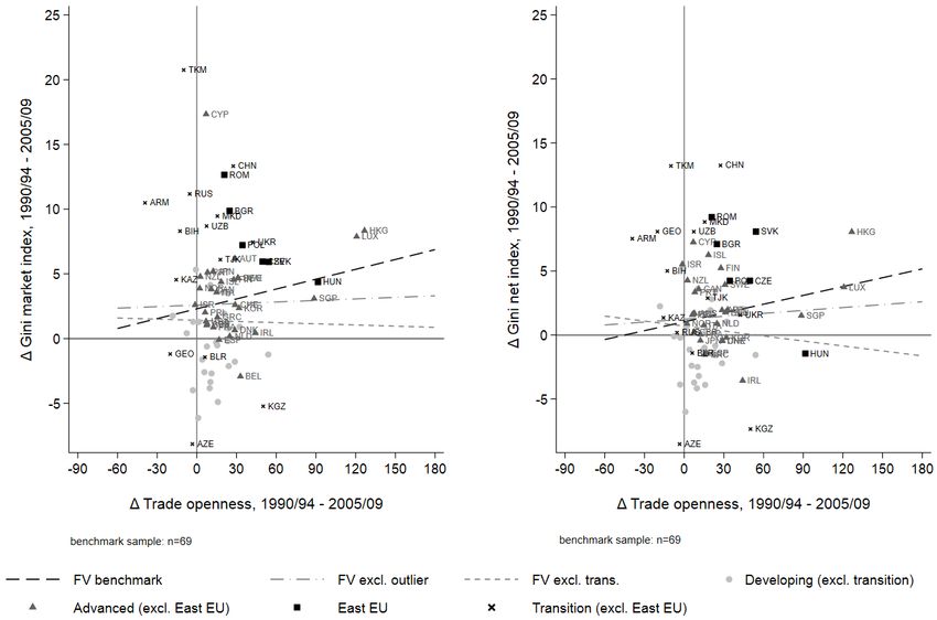
Imprint:

ifo Working Papers
Publisher and distributor: ifo Institute – Leibniz Institute for Economic Research at the
University of Munich
Poschingerstr. 5, 81679 Munich, Germany
Telephone +49(0)89 9224 0, Telefax +49(0)89 985369, email ifo@ifo.de
www.ifo.de

An electronic version of the paper may be downloaded from the ifo website:
www.ifo.de
ifo Working Paper No. 359

Trade Openness and Income Inequality: New Empirical Evidence*

                                               Abstract

We examine how trade openness influences income inequality within countries. The
sample includes 139 countries over the period 1970–2014. We employ predicted open-
ness as instrument to deal with the endogeneity of trade openness. The effect of trade
openness on income inequality differs across countries. Trade openness tends to dis-
proportionately benefit the relative income shares of the very poor, but not neces-
sarily all poor, in emerging and developing economies. In most advanced economies,
trade openness increased income inequality, an effect that is driven by outliers. Our
results suggest a strong effect of trade openness on inequality in China and transition
countries.

JEL Code: C26, D31, D63, F02, F60, H11, H20
Keywords: Trade openness, globalization, income inequality, instrumental variable
estimation, panel econometrics, development levels, transition economies

                  Florian Dorn**                                     Clemens Fuest
       ifo Institute – Leibniz Institute for              ifo Institute – Leibniz Institute for
               Economic Research                                  Economic Research
           at the University of Munich,                       at the University of Munich,
          University of Munich, CESifo                       University of Munich, CESifo
                 Poschingerstr. 5                                   Poschingerstr. 5
             81679 Munich, Germany                              81679 Munich, Germany
                   dorn@ifo.de                                        fuest@ifo.de

                                           Niklas Potrafke
                                ifo Institute – Leibniz Institute for
                                        Economic Research
                                    at the University of Munich,
                                   University of Munich, CESifo
                                          Poschingerstr. 5
                                      81679 Munich, Germany
                                          potrafke@ifo.de

This paper has been accepted for publication in Economic Inquiry.

* The authors have no conflicts of interest to declare. The article is independent research and partly
based on an earlier discussion paper conducted within the European Commission’s DG ECFIN Fellow-
ship Initiative 2016/17. The authors received funding from the European Commission during the Fel-
lowship Initiative 2016/17. FD received funding from the Hanns-Seidel-Foundation during this research.
** Corresponding author.
1 Introduction
How trade openness relates to income inequality has been examined in many empirical studies since the mid-1990s
(e.g., Wood, 1995; Cragg and Epelbaum, 1996; Feenstra and Hanson, 1996; Borjas et al., 1997; Leamer, 1998;
Meschi and Vivarelli, 2009; Jaumotte et al., 2013; Roser and Cuaresma, 2016). The empirical evidence is mixed.
These studies use macrodata at the country level and hardly report causal effects. We therefore investigate
how trade openness influences income inequality by employing a new identification strategy and considering
heterogeneity across countries. The sample includes up to 139 countries over the period 1970-2014.
We use an instrumental variable (IV) approach to identify the causal effect of trade openness on inequality.
Our IV is predicted openness based on a gravity equation using a time-varying interaction of geography and
exogenous large-scale natural disasters as proposed by Felbermayr and Gröschl (2013). The results do not suggest
that trade openness influences income inequality in the full country sample. There is a good reason why: The
Stolper-Samuelson theorem (Stolper and Samuelson, 1941) predicts that trade openness decreases inequality in
developing countries and increases inequality in developed countries.
We examine whether the effect of trade openness on income inequality differs across developing and developed
countries. In emerging and developing countries, our results suggest that trade openness disproportionately
benefits the very poor (not necessarily all poor), as predicted by the Stolper-Samuelson theorem. This finding is
in line with previous studies indicating that globalization, and in particular trade liberalization, reduces inequality
and poverty in developing countries (see Winters et al., 2004; Jaumotte et al., 2013; Bergh and Nilsson, 2014). In
our sample of 34 advanced economies, upper deciles disproportionately gain from trade openness at the expense
of the income shares of the bottom deciles of the income distribution. The relationship, however, is driven by
outliers. Our results therefore do not confirm, as predicted by the Stolper-Samuelson theorem, that trade openness
increases inequality in developed countries.
Our results, moreover, suggest a strong effect of trade openness on inequality within transition countries.
These countries have experienced a particularly fast change towards trade openness accompanied by large-scale
market-oriented reforms and an economic transition process in our period of observation. The market-oriented
reforms likewise promoted integration in the global market and increased income inequality. The impact on
income distribution during the transition period was hardly cushioned by either labor market institutions or
welfare states, which characterize many advanced economies (see Milanovic, 1999; Myant and Drahokoupil, 2010;
Perugini and Pompei, 2015b).
2 Theoretical predictions and empirical evidence
2.1 Theoretical predictions
The classical theoretical framework for examining the relationship between trade openness and distributional
market outcomes is the Heckscher-Ohlin (HO) model (Ohlin, 1933). It explains the inequality effect of trade
openness as a result of productivity differences and the relative factor endowment of countries, and the extent to
which individuals depend on labor or capital income. Countries specialize in production within their relatively
abundant factor and export these goods when they open up to trade. The Stolper-Samuelson theorem (Stolper
and Samuelson, 1941) shows that the subsequent trade-induced relative changes in product prices increase the
real return to the factors used intensively in the production of the factor-abundant export goods and decrease the
returns to the other factors. As a consequence, the country’s abundant production factors gain from openness,
while scarce factors lose. Because capital and skilled labor are relatively abundant in advanced economies, income
inequality and income concentration towards the top incomes is expected to increase. In developing countries,
unskilled labor, which is intensively used in local production, would benefit from economic openness by increasing
wages and income. In developing countries, income inequality is therefore expected to decrease. Based on the HO
model assumptions, how trade openness influences income inequality depends on a country’s development level.
Following the Stolper-Samuelson theorem, trade openness is expected to decrease income inequality in developing
countries and to increase income inequality in developed countries (with almost leveling effects in a full sample
including both groups).
Since the 1990s, several studies have pointed to limitations of the standard HO model implications and
provided mechanisms to explain why inequality patterns of country case studies do not necessarily follow the
predictions of the Stolper-Samuelson theorem. For instance, offshoring and outsourcing of less-skilled production
1decreases the wages and bargaining power of less-skilled workers in advanced economies, but offshored and out-
sourced activities might be relatively skill-intensive from the perspective of the workforce in developing countries
(see Feenstra and Hanson, 1996, 1999). Along the same lines, scholars discuss how rising exposure of sectors to
international trade competition (e.g., Cragg and Epelbaum, 1996; Munch and Skaksen, 2008; Egger and Kreick-
emeier, 2009; Sampson, 2014), import of capital goods (e.g., Feenstra and Hanson, 1997; Acemoglu, 2003), and
trade-induced technological transfers and catch-up processes (e.g., Berman and Machin, 2000; Zhu and Trefler,
2005; Burstein et al., 2013; Bloom et al., 2016) may increase the skill intensity and relative demand for skilled
labor in the developing world. In short, these mechanisms may explain why the skill premium of workers and
thus income inequality may rise in countries of all income groups when they opening to international trade.
2.2 Empirical evidence
How trade openness relates to income inequality has been examined in many empirical studies in the 1990s (e.g.,
Wood, 1995; Cragg and Epelbaum, 1996; Feenstra and Hanson, 1996; Borjas et al., 1997; Leamer, 1998) and has
been revisited since the early 2000s (e.g., Meschi and Vivarelli, 2009; Jaumotte et al., 2013; Roser and Cuaresma,
2016). The empirical evidence is mixed.1
Roser and Cuaresma (2016) use data for 32 developed countries and employ panel models over the period
1963-2002. They show that—in line with the Stolper-Samuelson theorem—trade openness is positively related to
income inequality. Their findings suggest that imports from developing countries are positively correlated with
income inequality in the developed world. This is a result that seems to be driven by the group of liberal market
economies but lacks statistical significance for other developed countries. The results by Meschi and Vivarelli
(2009) suggest, in contrast to the HO model predictions, that trade is positively associated with income inequality
in a sample of 65 developing countries. Their results are based on panel models over a rather short period from
1980 to 1999. The positive relationship between trade and income inequality within developing (Meschi and
Vivarelli, 2009) and within developed countries (Roser and Cuaresma, 2016) corroborates that international trade
gives rise to income inequality. By contrast, Jaumotte et al. (2013) suggest that trade openness is associated with
lower income inequality, a result that is based on a small sample of 31 developing and 20 developed countries
over the period 1981 to 2003. Their study does not, however, decompose the relationship between trade and
inequality within the subsamples of developing or developed countries. These empirical studies use macrodata at
the country level and hardly report causal effects.
Other studies use microdata to identify how trade openness influences local incomes across regions and workers
within individual countries. Empirical evidence on the effect with a focus on individual advanced economies is
mixed (e.g., Autor et al., 2013; Dauth et al., 2014). Reviews based on country case studies in the developing
world also conclude that the effect of trade on income inequality and poverty is context specific (e.g., Goldberg
and Pavcnik, 2007; Pavcnik, 2017). Microdata-based case studies are useful to understand causal mechanisms but
cannot predict external validity with respect to the overall effect of trade openness on income inequality.
Another strand of related studies examines the relationship of (economic) globalization and income inequality
(or poverty) (e.g., Dreher and Gaston, 2008; Bergh and Nilsson, 2010; Dorn and Schinke, 2018; Dorn et al., 2018;
Lang and Tavares, 2018; Sturm et al., 2019; Bergh et al., 2020).2 Overall, these studies find a positive relationship
between (economic) globalization and income inequality, although the results are mixed in advanced economies.
The findings, moreover, suggest a poverty-reducing effect of (economic) globalization in developing countries
(e.g., Bergh and Nilsson, 2010; Dorn et al., 2018; Lang and Tavares, 2018).3 These studies, however, often do not
decompose the effect of trade from financial indicators of economic globalization, and do not allow conclusions to
be inferred on the predictions of the HO trade model.4 We examine how trade openness influences inequality and
provide new empirical evidence on the HO theory predictions.5
1
Winters et al. (2004) review early empirical studies of the trade-inequality nexus and conclude that “there can
be no simple general conclusion about the relationship between trade liberalization and poverty” (p.106).
2
Some of these studies also use clever new identification strategies. For example, Lang and Tavares (2018) use
instrumental variables based on the geographical distribution of globalization.
3
Consequences of globalization are surveyed by Potrafke (2015).
4
There is no encompassing theory describing how overall (economic) globalization influences income inequality.
Scholars often use trade-based theories to describe how overall (economic) globalization influences income
inequality.
5
The same issue examined here was suggested, independently, by Siddique (2021).
23 Data
We use an unbalanced panel for up to 139 countries over the period 1970-2014. The data are averaged over five
years in nine periods between 1970 and 2014. We follow related literature and use five-year averages to reduce the
possibility of outliers, measurement errors, missing observations in individual years and short-term movements in
the business cycle influencing the inferences (see Felbermayr and Gröschl, 2013).
3.1 Variables
Income inequality
We use the Gini household income inequality indices of Solt’s (2016) Standardized World Income Inequality
Database (SWIID, v5.1) as the primary measure of income inequality. SWIID provides standardized Gini income
inequality measures for market and net outcomes based on the same concept, and thus allows the comparison of
income inequality before and after redistribution by taxation and transfers over time. We use both the market
and net income Gini indices.
The high coverage across countries and time and the adjustment procedure for achieving possible comparabil-
ity is the major reason for preferring SWIID to other secondary source datasets (see Dorn, 2016, for a discussion).
SWIID uses the Luxembourg Income Study (LIS) as a baseline. To predict missing observations in the LIS se-
ries, data from other secondary data sources and statistical offices are standardized to LIS by using systematic
relationships of different Gini types and model-based multiple imputation estimates. When estimating missing
observations, Solt (2016) considers that adjustments cannot be constant across countries and time by relying on
information from proximate years in the same country as the best solution, and on information on countries in
the same region and with similar development level as the second-best solution. There are, however, concerns
over the reliability of SWIID’s imputed estimates in data-poor regions (Ferreira et al., 2015; Jenkins, 2015).
A shortcoming of Gini indices is that they do not show which parts of a country’s income distribution
disproportionately gain or lose and cause changes in the Gini index. We therefore also employ the released data
on relative net income shares of the Global Consumption and Income Project (GCIP) by Lahoti et al. (2016) as
a measure of post tax and transfer income inequality. In a similar vein as SWIID, they estimate standardized
measures based on the available data sources to increase comparability across countries and time, and increase
the coverage of the data by using interpolation methods for missing country-year observations.
Trade openness and covariates
We measure trade openness by the sum of imports and exports as a share of GDP. Trade data are taken from the
World Development Indicators (World Bank, 2017).
We include the following control variables: real GDP per capita to control for any distributional effect due
to different income levels. Economic growth and the GDP per capita level have been shown to be positively
related to globalization and international trade (see Dreher, 2006; Dreher et al., 2008; Feyrer, 2009; Felbermayr
and Gröschl, 2013; Gygli et al., 2019) and to the development of the income distribution over time (see Berg et al.,
2012). Demographic changes and shifts in the size of population are also likely to influence both international trade
and the income distribution (OECD, 2008). We therefore add the age dependency ratio and the logarithm of total
population. The dependency ratio measures the proportion of dependents per 100 of the working age population,
where citizens younger than 15 or older than 64 are defined as the dependent (typically non-productive) part. A
higher share of dependent citizens is usually associated with higher income inequality and higher redistribution
activities within countries. Shifts in the size of the population affect the dependency ratio as well as a country’s
labor and skill endowment. Trade openness is likely to be correlated with other indicators of globalization such
as FDIs, migration or political globalization. Other globalization indicators might also influence inequality within
countries (Borjas et al., 1997; Bergh and Nilsson, 2010; Jaumotte et al., 2013; Dorn et al., 2018; Lang and
Tavares, 2018; Sturm et al., 2019). We therefore use the KOF globalization subindices for political and social
globalization as well as an index for FDIs as controls in our baseline models (Dreher, 2006, update KOF 2016).
Our instrument predicted openness is constructed by using a gravity model including exogenous large-scale natural
disasters in other countries. Natural disasters themselves are shown to influence trade openness and the per capita
income level of countries (see Felbermayr and Gröschl, 2013, 2014). Some natural disasters are registered across
borders. Natural disasters registered in the home country might have a direct impact on the home country’s
income distribution (see Keerthiratne and Tol, 2018). To make sure that our estimated relationship between
trade and inequality is not driven by the correlation between disasters registered in the home country and income
3inequality, we directly control for the effect of large-scale natural disasters on the income distribution within
countries. We included the one-period lagged large-scale natural disasters as a baseline control variable. Table
A1 in the Appendix describes summary statistics and data sources of all variables.
3.2 Country subsamples
Full and benchmark samples
Next to our full sample of 139 countries, we also use a sample for high and upper middle income countries as our
benchmark sample. High and upper middle income countries are classified by the criterion of the World Bank as
of 2015 and include 82 countries having a gross national income (GNI) per capita of USD 4,126 or more. The
57 countries in our dataset below the GNI per capita threshold of USD 4,126 are classified as low income and
lower middle income countries (lower income countries). Lower income countries are more likely than high and
middle income countries to have few period observations per country due to a lack of data availability. Data in
lower income countries are, moreover, more likely to be subject to measurement errors. There are serious concerns
about the quality of the income inequality data from less developed countries. Jenkins (2015), for example, shows
that source data on inequality of high quality, in which the income concept and the survey can be verified, are
rare in less developed and in particular in sub-Saharan African countries. The lack of data quality is also reflected
in the imputed Gini estimates in SWIID, as the imputation variability of imputed country-period observations
is large in some countries, especially in lower income countries (Ferreira et al., 2015; Jenkins, 2015). To address
potential biases in the estimates because of data quality, our benchmark sample excludes the 57 lower income
countries that are in the full sample. 29 of the 57 excluded countries are sub-Saharan African countries.
Development levels
We use subsamples for the most advanced economies and emerging markets & developing economies (EMD).6 To
distinguish between advanced economies and emerging markets and developing economies we apply the classifi-
cation of the International Monetary Fund (IMF, 2016). This classification is based on per capita income levels.
However, it also considers export diversification and the degree of integration into the global financial system
to classify advanced economies.7 The 34 countries fulfilling the criterion of the advanced economies sample are
also included in our benchmark sample (high and upper middle income countries). The subsample of emerging
markets and developing economies includes 105 countries taken from both income groups, the full set of lower
income countries and the countries of the benchmark sample, which are not classified as advanced economies.
Transition economies
Transition economies are another important country sample when examining the trade openness-inequality nexus.
Transition economies have experienced a large shift in trade openness since the fall of the Iron Curtain. The global-
ization shock for transition countries was, however, hardly cushioned by either labor market institutions, education
systems or welfare states, which characterize many advanced economies in the rest of the world. The transition
countries had limited capabilities in the education system and higher labor market frictions at the beginning of
their transition. The education and social systems rather deteriorated in the transition period (e.g., Campos
and Coricelli, 2002). The transition to an open and competitive market economy, FDI-induced new technologies
and equipment, and the overall skill-biased technological shift in the 1990s suddenly required other skills than
the working age population and the education systems were prepared for (see Aghion and Commander, 1999).
During the simultaneous period, transition countries also experienced many structural and institutional changes
in political institutions and their economy, such as privatizations of state-owned enterprises, deindustrialization,
price liberalizations, financial development, labor and product market deregulation, new models of corporate
governance, or shrinking and reforming of the public sector during their transformation from centrally planned
to market-based economies (Milanovic, 1999; Roland, 2000; Flemming and Micklewright, 2000; Ivanova, 2007;
Myant and Drahokoupil, 2010; Perugini and Pompei, 2015b). One of the most visible outcomes of the systematic
change and complex interplay of several forces is a remarkable increase in income inequality (see Campos and
Coricelli, 2002; Ivanova, 2007; Perugini and Pompei, 2015a). The market-oriented reforms, moreover, promoted
the inflow of FDI and the countries’ integration in the global market. The transition toward market economies
might therefore be an omitted driver of trade openness and inequality in transition countries. The systemic change
6
See Appendix for the list of countries by development levels.
7
Several oil exporters that have high per capita GDP but almost no export diversification, for example, would
not make the IMF classification for advanced economies.
4and restructuring of the economy and governance has likely influenced the speed of globalization and the rise of
income inequality (Milanovic, 1999; Milanovic and Ersado, 2011; Aristei and Perugini, 2014).
We use a sample of the (new) European Union member states from Central and Eastern Europe (East EU)
and China. These countries have already been shown to contribute to a large extent to changes in the global
income distribution since the fall of the Berlin Wall (see Lakner and Milanovic, 2016).
4 Descriptive statistics
4.1 Trade openness and income inequality across countries
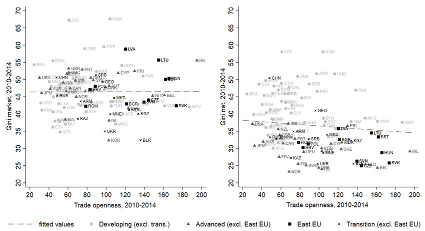
We examine the correlation between trade openness and income inequality across countries in the most recent
five-year period of observation, 2010-2014: Income inequality before taxes and transfers is hardly correlated with
trade openness (see Figure 1). The coefficient of correlation is 0.01.
The Gini index after tax and transfers is on average 9.8 index points lower than the Gini index value before
redistribution in the period 2010-14. Net income inequality in open countries is, however, lower than in less open
countries. The correlation coefficient between trade openness and the Gini net index is -0.17, indicating that more
developed and open countries have larger welfare states. EU member states and other advanced economies are
among the most open countries and have the world’s lowest levels of income inequality after redistribution.
Figure 1: Trade openness and Gini income inequality, 2010-2014
Source: SWIID 5.1, World Bank (2017), own calculations.
Notes: Figure 1 relates to the full country sample within the period 2010-2014. The figure excludes Luxem-
bourg and Singapore as outliers. Transition (excl. East EU) relate to former members of the Soviet Union
(FSU, non-EU), Western Balkan (non-EU) states, and China. Unconditional correlations: βmarket = 0.005;
βnet = −0.171∗ (∗ p < 0.1).
4.2 Trends across samples and countries
Trade openness and income inequality both increased quite rapidly between the late 1980s and the late 1990s;
that is the first decade after the fall of the Berlin Wall in 1989 (Figure 2). There was a further increase in
trade openness around the world in the 2000s. The pre tax/transfer and post tax/transfer Gini indices, however,
decreased from the early 2000s in EMD economies. In advanced economies, the Gini net index has been around
31 since 2000, while market income inequality has increased in the same period of time. The differing trends in
the mean values of the Gini indices before and after taxation and transfers indicate a rise of redistribution in
the sample of advanced economies since the early 2000s. Before taxation and transfers, income inequality is at a
5similar level in advanced and EMD economies. After taxation and transfers, inequality is much lower in advanced
economies than in the emerging and developing world.8
Figure 2: Global trends in trade openness and Gini income inequality
Source: SWIID 5.1, World Bank (2017), own calculations.
Notes: Trends between the periods 1985-1989 and 2010-2014. Unweighted mean of balanced samples. In
the full sample, 63 of 140 countries have observations in all six periods, in the benchmark sample 47 of 82
countries, 24 of 34 countries within the sample of advanced economies, and 39 of 106 countries in the sample
of emerging and developing economies (EMD).
In Figure 3 we focus on changes in income inequality and trade openness in individual countries of our
benchmark sample between the periods 1990-1994 and 2005-2009 (based on 69 countries from the benchmark
sample having observations in both periods 1990-1994 and 2005-2009). The unconditional correlation between
the changes in trade openness and the market and net income inequality is positive. The coefficients of correlation
are 0.025 and 0.023. There are, however, two groups of countries that are the key drivers of the linear relationship
between the late 1980s and late 2000s: First, Hong Kong, Luxembourg and Singapore are outliers regarding
trade openness. Second, the transition countries in Eastern Europe and China experienced a huge opening
process (globalization shift) and a huge rise in income inequality during that time.9 The other countries from
the benchmark sample also enjoyed rapidly increasing trade openness but experienced less pronounced increases
in income inequality than Eastern European countries and China. When we exclude the outliers Hong Kong,
Luxembourg and Singapore, the unconditional correlation between the change in trade openness and income
inequality is almost zero (the coefficients are 0.004 and 0.008). After excluding outliers and transition countries,
the unconditional correlation between the change in trade openness and income inequality is negative instead.
The coefficients of correlation are -0.003 and -0.013 when we exclude transition countries and outliers from
the benchmark sample. Within the sample of advanced economies, the changes in trade openness and income
inequality outcomes are hardly correlated between the periods 1990-1994 and 2005-2009. The coefficients of
correlation are 0.027 and 0.024. After excluding transition countries and outliers, the relationship between trade
and the Gini inequality indices turns out to be negative. The coefficients of correlation are -0.072 and -0.078 in
the remainder sample of advanced economies.
8
In the EU15, post tax/transfer inequality is lower than in other advanced regions such as the western offshores.
The trends in inequality reflect the fact that countries of the western offshores such as the United States do
have more market-oriented economic systems and less generous welfare states than their Scandinavian and
continental European counterparts (see Fuest et al., 2010; Doerrenberg and Peichl, 2014; Dorn and Schinke,
2018). Empirical research has shown how inequality dynamics differ among advanced economies during the last
wave of globalization, with larger increases in income inequality in Anglo-Saxon countries such as the United
States and less pronounced trends in Continental Europe (see Atkinson and Piketty, 2007; Dorn, 2016; Roser
and Cuaresma, 2016; Dorn and Schinke, 2018).
9
Post-communist countries from Central and Eastern Europe (East EU) and the former Soviet Union (FSU) had
relatively low levels of trade openness and income inequality before 1990. During their first stage of transition
from centrally planned to market-based economies in the 1990s, both groups experienced a large rise in trade
openness and income inequality (see Dorn et al., 2018). While trade openness increased in both groups during
the 2000s, inequality increased in new EU member countries from Central and Eastern Europe but decreased
in the other countries of the former Soviet Union such as the Russian Federation (see Gorodnichenko et al.,
2010; Aristei and Perugini, 2014).
6Figure 3: Changes in trade openness and Gini income inequality, between 1990/94 and 2005/09
7
Source: SWIID 5.1, World Bank (2017), own calculations.
Notes: Figure 3 describes countries within the benchmark sample including high and middle income countries having observations in periods
1990-1994 and 2005-2009. Transition (excl. EU) captures former members of the Soviet Union, Western Balkan (Non-EU) states, and China.
The balanced benchmark sample includes 69 countries. Hongkong, Luxembourg and Singapore are extreme outliers. After excluding outliers and
transition countries, the balanced sample consists of 52 countries. Unconditional correlations in the benchmark sample: βmarket = 0.025, βnet =
0.023, after excluding outliers βmarket = 0.004, βnet = 0.008, and after excluding outliers and (EU and Non-EU) transition economies βmarket =
−0.003, βnet = −0.013; significance level: ∗ p < 0.1. FV = fitted values.5 Empirical strategy
5.1 OLS panel fixed effects model
We estimate the baseline panel model by ordinary least squares (OLS), where countries are described by i and
five-year periods by τ :
0
Yi,τ = β × T RADEi,τ + Θ × χi,τ + υi + υτ + i,τ (1)
Yi,τ describes the measure of income inequality (Gini index, or relative income share by decile) of country i in
period τ . The explanatory variable T RADEi,τ describes the trade openness of country i in period τ . The vector
χi,τ includes control variables as described in Section 3.1, υi describes the country fixed effects, υτ describes the
fixed period effects, and i,τ is the error term. All variables are included as averages in each of the nine periods
(t = 1,...,9).
By estimating OLS in a fixed effects (FE) model we exploit the within-country variation over time, eliminating
any observable and unobservable country-specific time-invariant effects. We also include fixed time effects to
control for other confounding factors (e.g., period-specific shocks) that influence multiple countries simultaneously.
We use standard errors robust to heteroscedasticity clustered at the country level.
5.2 2SLS panel IV model
Endogeneity problem and IV approach
There are two reasons for potential endogeneity of trade openness in our model: omitted variable bias and reverse
causality.
We included many control variables, but other unobserved omitted variables may give rise to biased estimates.
The omitted variable bias indicates that there is still a third (or more) variable(s), which influence(s) both trade
openness and income inequality. For example, increasing mobility may induce countries to reduce (capital) taxes
and cut welfare benefits, which, in turn, will influence disposable income and probably also employment. If
competition from countries with cheap labor induces companies in high income countries to specialize in the
production of high-tech goods and services, which requires highly skilled labor, this will have an impact on the
skill premium. It is difficult to disentangle these effects from the ‘direct’ influence of trade openness on income
inequality, that is the influence of trade openness, given other factors.
Second, reverse causality may occur because changes in income inequality are likely to influence policies that
affect trade openness. The debate on the Transatlantic Trade and Investment Partnership (TTIP), for instance, is
also influenced by the perception that gains from trade may be distributed rather unevenly. Shifts in the income
distribution within a country may also have direct effects on the trade openness level of the country, for example
if more people are able to travel, to buy more expensive import goods or to make international investments and
savings.
To deal with the endogeneity problem of trade openness, we use predicted openness based on a gravity
equation as an IV. Frankel and Romer (1999) apply predicted openness in a cross-sectional approach. We want
to exploit exogenous time variation in predicted openness using the IV in a panel model and controlling for
unobserved country effects (see Feyrer, 2009; Felbermayr and Gröschl, 2013). We employ the exogenous component
of variations in openness predicted by geography and time-varying natural disasters in foreign countries, as
proposed by Felbermayr and Gröschl (2013) for a panel data model, as an IV for trade openness. The incidence of
natural disasters such as earthquakes, hurricanes or volcanic eruptions in one country influences the openness of
its trading partners, depending on the two countries’ geographic proximity.10 An earthquake hitting Mexico, for
example, will increase international trade of other countries with Mexico. The rise in a country’s trade openness
level will be larger, the closer a country is located to Mexico.
Instrument construction
The predicted openness is constructed in two steps: First, exogeneous natural disasters are included in a gravity
model to predict bilateral trade openness. Bilateral openness ω̂ti,j describes trade flows between country i and
10
For example, the effect of an earthquake in Mexico will be stronger for trade flows of Honduras or the United
States than those of India.
8country j in year t and is predicted by a reduced gravity model using a Poisson Pseudo Maximum Likelihood
(PPML) estimation to account for zero trade flows and standard errors clustered by country pairs.
Bilateral openness ω̂ti,j is regressed on variables exogenous to income inequality such as largescale natural
disasters in foreign countries j, interactions of the incidence of natural disasters in foreign countries j and bilateral
geographic variables, or population:
0 0
ω̂ti,j = exp[δ × Dtj + γ × Zti,j + λ × (Φi,j j i j i,j
t × Dt ) + υ + υ + υt + t ] (2)
where Zti,j = [lnP OPti ; lnP OPtj ; lnDIST i,j ; BORi,j ] includes exogenous controls such as population (P OP )
in countries i and j in year t, and the bilateral geographic variables distance DIST , and a common border dummy
BOR, based on Frankel and Romer (1999). Dtj denotes exogenous large-scale natural disasters in country j, while
Φi,j j j j i,j
t = [lnF IN DISTt ; lnAREA ; lnP OPt ; BOR ] describes the exogenous variables interacting with Dt , such
j
as the international financial remoteness F IN DIST , the surface area AREA, or population P OP of country j.11
Country and time fixed effects are captured by υ i , υ j , υt , while i,j
t accounts for the idiosyncratic error. The
bilateral openness equation (2) is designed to maximize conditional correlation between observed trade openness
and the constructed instrument (see relevance of the instrument below).
We follow the approach preferred by Felbermayr and Gröschl (2013) and use exogenous “large” scale natural
disasters (as Dtj ) to make sure that a disaster is of a sufficiently large dimension and caused not by local deter-
minants or the development level of the country but rather by exogenous global phenomena. This classification
of natural disasters includes “large” earthquakes, droughts, storms, storm floods and volcanic eruptions that (i)
caused 1,000 or more deaths; or (ii) injured 1,000 or more people; or (iii) affected 100,000 or more people. In
our robustness checks, we use alternative definitions of disasters to construct the instrument, such as a broader
specification of disasters that includes all kinds of natural disasters or counting all sizes of disasters (see Section
6.4). The data on natural disasters is taken from the Emergency Events database (EM-DAT).
In the second step of constructing the IV, Felbermayr and Gröschl (2013) use an exogenous proxy for mul-
tilateral openness Ωi,t by aggregating the obtained predicted bilateral openness values ω̂ti,j of country i over all
bilateral country pairs and years t:
X
Ωi,t = ω̂ti,j (3)
i6=j
Based on our underlying data, we obtain values for all years from 1966 to 2008. Averaging over nine periods
τ and using one-period lags of predicted openness Ωi,τ −1 , we obtain our instrument for T RADEi,τ in equation
(1).
Relevance of the instrument
The relevance of the IV predicted openness Ωi,τ −1 depends on its conditional correlation with trade openness
T RADEi,τ . The first stage regression has the following form:
0
T RADEi,τ = α × Ωi,τ −1 + ϕ × χi,τ + υ j + υt + i,j
t (4)
The model is estimated by applying the FE estimator, controlling for any time-invariant country character-
istics, and using robust standard errors clustered at the country level. The first stage also includes all control
variables χi,τ as in equation (1) and period dummies to control for common period effects.
The first stage regression results show that the IV is relevant (see Appendix, Table A2). Our predicted
openness variable correlates positively with trade openness (T RADE). The relationship is statistically significant
at the 1% level in the full sample, the benchmark sample and in the sample of advanced economies. In the sample
of developing economies, the statistical significance is at the 10% level. The Cragg-Donald Wald F-statistics on
the excluded instrument are well above the 10% critical value (F ≥ 16.38) of the weak instrument test by Stock
and Yogo (2005). The partial R2 of lagged predicted openness ranges between 2.4% in the sample of developing
economies and 23.3% in the sample of advanced economies.
Exclusion restriction
Income inequality does not influence predicted openness because the instrument is constructed from exogenous
11
As large-scale natural disasters may hit both bordering countries, the interaction of disasters and the common
border dummy is included. Interactions of the disaster variable with surface area and population in country j
consider the fact that economic and population density matters for the aggregate damage caused by large-scale
natural disasters.
9components, such as large-scale natural disasters and bilateral geographic components. We do not believe that
predicted openness influences income inequality directly or through other explanatory variables that we did not
include in our model. Predicted openness is an arguably excludable instrument. Foreign natural disasters are
expected to have no effect on income inequality other than through the extent of trade openness or other indicators
of globalization, e.g., international transactions and migration. We control for other globalization indicators such
as FDIs and social and political globalization in our regression models. Migration is included in the social
globalization index and we control for migration as an individual variable in our robustness tests.12
Large-scale natural disasters may give rise to changes in the income distribution. Felbermayr and Gröschl
(2013, 2014) have shown, for example, that natural disasters influence overall per capita income. Some natural
disasters are registered across borders. Natural disasters registered in the home country might have a direct
impact on the home country’s income distribution (see Keerthiratne and Tol, 2018). To mitigate any potential
omitted variable bias because of cross-border natural disasters we directly control for the effect of large-scale
natural disasters in the home country.
6 Results
6.1 Baseline results
We examine the average effect of trade openness on Gini income inequality in our full and benchmark sample.
Our results in Table 1 do not suggest a statistically significant relationship between trade openness and income
inequality in the full sample and benchmark sample—estimating the models by OLS (columns 1-4) and 2SLS
(columns 5-8) notwithstanding. The baseline specifications do not confirm that trade openness influences in-
equality within countries when we use large country samples—in line with predictions of the Stolper-Samuelson
theorem.
The baseline results in Table 1 also show the coefficient estimates of the control variables. FDIs and large-
scale natural disasters increase income inequality both before and after redistribution. The Gini market index
increases when the share of dependents increases. Population and inequality are negatively correlated before tax
and transfers.
Table 2 shows the baseline 2SLS results when we use the relative net income shares (by deciles) as the
dependent variables. The results in Table 2 corroborate our baseline results when using the Gini index as the
dependent variable in the full sample (panel a), indicating that the relationship between trade openness and
income inequality lacks statistical significance. The relationship between trade openness and relative income
shares in the benchmark sample is more pronounced (panel b). The coefficient estimate of trade openness is
negative when the relative income shares of the lower income deciles 1 to 7 are used as the dependent variables
and positive when the relative income shares of the three highest income share deciles are used as the dependent
variables. But the coefficient estimates are rather small. The effect of trade openness, however, is only statistically
significant for the upper middle class in the 9th decile (column 9 of Table 2). The coefficient is significant at
the 5% level and indicates that the income share of decile (9) increased by 0.12 percentage points when trade
openness increased by ten percentage points.
6.2 The role of development levels
The effect of trade openness on income inequality is expected to differ depending on the development level of
countries. The Stolper-Samuelson theorem (Stolper and Samuelson, 1941) predicts that trade openness increases
inequality in developed countries and decreases inequality in developing countries. We examine two subsamples
depending on the development level of countries: the sample of 34 advanced economies and the sample of 102
emerging markets and developing economies (see Table 2, panel c and d). The instrument is relevant within both
subsamples. The Cragg-Donald Wald F-statistic is above the 10% and 15% critical values.
12
One may argue that the exclusion restriction is not fulfilled because natural disasters that occur in the trading
partner countries (which are often direct geographical neighbors) give rise to migration. For example, when a
natural disaster occurs in Mexico, especially poor Mexican citizens are likely to leave Mexico and migrate to a
neighboring country such as Honduras. If this is true, the natural disaster that hit Mexico (and gave rise to
the exogenous variation in our instrumental variable predicted openness) influenced trade openness and income
inequality in Honduras. Empirical studies show, however, that natural disasters hardly give rise to international
migration in the medium and long term (see Gröschl and Steinwachs, 2017).
10Table 1: Trade openness and income inequality – baseline results (OLS and 2SLS)
OLS 2SLS
Full sample Benchmark sample Full sample Benchmark sample
(1) (2) (3) (4) (5) (6) (7) (8)
Gini market Gini net Gini market Gini net Gini market Gini net Gini market Gini net
Trade openness 0.00817 0.0110 -0.00872 -0.00107 -0.0658 -0.0276 0.000943 0.0232
(0.0133) (0.0106) (0.0153) (0.0113) (0.0692) (0.0563) (0.0418) (0.0339)
GDP p.c. 0.0952 0.0235 0.0955 0.00434 0.150 0.0522 0.0880 -0.0146
(0.0590) (0.0500) (0.0575) (0.0460) (0.0916) (0.0673) (0.0743) (0.0517)
Population (log) -5.322∗ -2.298 -2.873 1.146 -5.964∗∗ -2.633 -2.660 1.682
(2.835) (2.203) (3.969) (3.075) (2.842) (2.204) (3.858) (3.186)
Age dependency 0.129∗∗ 0.0666 0.193∗∗∗ 0.140∗∗ 0.101 0.0518 0.197∗∗∗ 0.151∗∗∗
(0.0509) (0.0436) (0.0692) (0.0597) (0.0613) (0.0513) (0.0683) (0.0578)
Social glob. 0.0618 0.0252 0.0431 0.000700 0.0604 0.0245 0.0435 0.00156
11
(0.0507) (0.0400) (0.0522) (0.0399) (0.0498) (0.0375) (0.0508) (0.0407)
Political glob. -0.0346 -0.0173 -0.0102 0.00560 -0.0212 -0.0103 -0.0131 -0.00176
(0.0369) (0.0303) (0.0464) (0.0379) (0.0395) (0.0312) (0.0467) (0.0377)
FDI 0.0695∗∗∗ 0.0426∗∗∗ 0.0777∗∗∗ 0.0437∗∗∗ 0.0783∗∗∗ 0.0472∗∗∗ 0.0777∗∗∗ 0.0437∗∗∗
(0.0208) (0.0154) (0.0260) (0.0162) (0.0222) (0.0168) (0.0254) (0.0159)
Nat. disasters (t-1) 2.103∗∗∗ 2.115∗∗∗ 2.390∗∗∗ 2.450∗∗∗ 2.255∗∗∗ 2.194∗∗∗ 2.377∗∗∗ 2.419∗∗∗
(0.377) (0.478) (0.315) (0.392) (0.345) (0.445) (0.317) (0.403)
Fixed effects
Country FE Yes Yes Yes Yes Yes Yes Yes Yes
Period FE Yes Yes Yes Yes Yes Yes Yes Yes
Countries 139 139 82 82 139 139 82 82
Observations 794 794 516 516 794 794 516 516
Partial R2 0.067 0.131
F Test, weak ID 45.573 62.899
F Test, p-value 0.000 0.000
Notes: OLS and 2SLS panel fixed effects estimations based on nine periods using 5-year averages between 1970 and 2014. Clustered robust standard errors in
parentheses. Weak ID test using Cragg-Donald Wald F-statistic. Stock and Yogo (2005) weak ID critical value: 16.38 (10 %). Significance levels: ***p < 0.01; **p
< 0.05; *p < 0.1.Table 2: Trade openness and income inequality – subsample results (2SLS)
(1) (2) (3) (4) (5) (6) (7) (8) (9) (10) (11) (12)
(13)
D1 D2 D3 D4 D5 D6 D7 D8 D9 D10 Gini market Gini net
(a) Full sample
Trade openness -0.000703 -0.00229 -0.00168 -0.000640 0.000542 0.00174 0.00288 0.00384 0.00442 -0.00835 -0.0666 -0.0284
(-0.08) (-0.29) (-0.23) (-0.09) (0.08) (0.30) (0.57) (0.78) (0.51) (-0.20) (-0.97) (-0.51)
Countries 136 136 136 136 136 136 136 136 136 136 136 136
Observations 783 783 783 783 783 783 783 783 783 783 783 783
Partial R2 0.067
F Test, weak ID 45.593
F Test pvalue 0.000
(b) Benchmark sample
Trade openness -0.00707 -0.00861 -0.00826 -0.00735 -0.00600 -0.00411 -0.00137 0.00302 0.0117∗∗ 0.0280 0.000222 0.0228
(-1.02) (-1.41) (-1.47) (-1.42) (-1.28) (-0.99) (-0.37) (0.81) (2.00) (0.89) (0.01) (0.68)
Countries 81 81 81 81 81 81 81 81 81 81 81 81
Observations 513 513 513 513 513 513 513 513 513 513 513 513
Partial R2 0.134
F Test, weak ID 64.572
F Test pvalue 0.000
(c) Advanced econ.
12
Trade openness -0.00867∗∗ -0.00779∗ -0.00667 -0.00537 -0.00382 -0.00191 0.000522 0.00389 0.00942∗∗∗ 0.0204 -0.0287 0.00350
(-2.12) (-1.94) (-1.51) (-1.14) (-0.81) (-0.42) (0.13) (1.28) (2.88) (0.69) (-0.79) (0.16)
Countries 34 34 34 34 34 34 34 34 34 34 34 34
Observations 244 244 244 244 244 244 244 244 244 244 244 244
Partial R2 0.233
F Test, weak ID 58.875
F Test pvalue 0.000
(d) Developing econ.
Trade openness 0.0317∗ 0.0240 0.0219 0.0203 0.0183 0.0148 0.00900 -0.00151 -0.0231 -0.117 -0.235 -0.212
(1.71) (1.41) (1.25) (1.13) (1.03) (0.88) (0.61) (-0.12) (-1.07) (-1.04) (-1.09) (-1.14)
Countries 102 102 102 102 102 102 102 102 102 102 102 102
Observations 539 539 539 539 539 539 539 539 539 539 539 539
Partial R2 0.025
F Test, weak ID 10.821
F Test pvalue 0.072
Notes: 2SLS panel fixed effects estimations based on nine periods using 5-year averages between 1970 and 2014. T-statistics in parentheses. Robust standard errors
clustered at the country level. All specifications include country and year fixed effects, and baseline control variables (see Table 1): GDP per capita, population(log),
dependecy ratio, social globalization index, political globalization index, FDI index, and large scale natural disasters. Weak ID test using Cragg-Donald Wald F-
statistic. Stock and Yogo (2005) weak ID critical values: 16.38 (10 %), 8.96 (15 %). Significance levels: ***p < 0.01; **p < 0.05; *p < 0.1.We examine how trade openness influences Gini inequality. 2SLS results in Table 2 do not show that trade
openness influences income inequality when we use Gini market and Gini net indices as the dependent variables
(columns 11-12), neither within the most advanced economies (panel c) nor within the sample of emerging and
developing economies (panel d).
We also examine how trade openness influences the relative net income shares in Table 2 (columns 1-10).
Within the advanced economies, the results suggest that trade openness increased income inequality. Table 2
shows that trade openness decreased the relative net income shares of the lowest income deciles and increased
the relative net income shares of the upper middle class income deciles (panel c). The effect is negative and
significant for the two lowest income deciles (panel c, columns 1-2) and positive and statistically significant for
the 9th decile (panel c, column 9). The coefficient, however, indicates a rather small effect. The income share
of the upper middle class (decile 9) increased by 0.09 percentage points when trade openness increased by 10
percentage points. Within the emerging and developing world, our results suggest that trade openness tends to
decrease income inequality. Trade openness tends to decrease income shares of the upper deciles and to increase
income shares of the poor and middle class within the emerging and developing economies. Trade openness,
however, also lacks statistical significance in almost all specifications in Table 2, panel (d). The exception is the
coefficient estimate in panel (d), column (1), suggesting a rather positive effect of trade openness on the relative
income share of the poorest in the income distribution of emerging and developing countries. The coefficient
indicates that the bottom 10% income share (decile 1) increased by 0.3 percentage points when trade openness
increased by 10 percentage points.
Our 2SLS results based on relative income shares as the dependent variable are again in line with predictions
of the Stolper-Samuelson theorem. Within developing economies, our findings suggest that the poorest people
disproportionately gain from trade openness at the expense of the relative income shares of higher income deciles.
Within advanced economies, our findings suggest that the upper middle class disproportionately gain from trade
openness at the expense of the relative income shares of bottom deciles.
The findings suggest that trade openness influences income inequality, both within our benchmark country
sample and within advanced economies. The benchmark sample includes the advanced economies sample and the
48 emerging economies having a per capita income level above a minimum threshold (not including developing
countries having a GNI per capita below USD 4,126, as of 2015). As coefficient estimates of trade openness in
the benchmark sample are larger than in the sample of advanced economies, and 41.5 percent of countries in
the benchmark sample are advanced economies, other countries within the benchmark sample might be the main
drivers of the significant positive effect of trade openness on income inequality.
6.3 Outliers and transition countries
The unconditional relationship between the change in trade openness and income inequality seems to be driven
by outliers in trade openness and by Central and Eastern European transition countries (East EU) and China
(see Section 4). We therefore examine the effect of trade openness on income inequality when we exclude outliers
and transition countries. The results are shown in Table 3.
First, we exclude Singapore as an outlier in trade openness from the sample of advanced economies (Table 3,
panel a) and the benchmark sample of high and upper middle income countries (Table 3, panel b). The results
in Table 3 show that all coefficient estimates lack statistical significance after excluding Singapore, both in the
advanced economies and in the benchmark sample. Within the remaining 33 advanced economies, the coefficient
estimates for trade openness are positive for the effect on the bottom 70% income share (panel a, columns 1-7)
and negative for the effect on income shares of the upper 30% (panel a, columns 8-10) after excluding the nine
observations for Singapore. Within the remaining benchmark sample of 80 countries, the coefficient estimates for
trade openness have are positive for the bottom 20% and top 20% income shares (panel b, columns 1-2 and 9-10)
and negative for the deciles in the middle class (panel b, columns 3-8) after excluding observations for Singapore.
These findings, however, do not support the prediction by the Stolper-Samuelson theorem that trade liberalization
increases inequality in developed countries.
Second, we exclude China and the East EU transition countries from the benchmark sample of high and
upper middle income countries (Table 3, panel c). The coefficients of the trade openness variables become smaller
and do not turn out to be statistically significant when we exclude China and the East EU transition countries.
After excluding China and transition economies, the coefficient estimate of trade openness on the income share
of the 9th decile in column (9) is 0.008 and lacks statistical significance—it is 0.012 at the 5% significance level
when China and transition economies are included (Table 2, panel b). In a similar vein, the coefficient of trade
13Table 3: The role of outliers and transition economies (2SLS)
(1) (2) (3) (4) (5) (6) (7) (8) (9) (10) (11) (12)
(13)
D1 D2 D3 D4 D5 D6 D7 D8 D9 D10 Gini market Gini net
(a) Advanced, excl. outlier
Trade openness 0.00728 0.00503 0.00386 0.00304 0.00231 0.00150 0.000403 -0.00131 -0.00432 -0.0178 -0.0306 -0.000956
(0.95) (0.72) (0.55) (0.44) (0.36) (0.26) (0.08) (-0.27) (-0.60) (-0.44) (-0.49) (-0.03)
Countries 33 33 33 33 33 33 33 33 33 33 33 33
Observations 235 235 235 235 235 235 235 235 235 235 235 235
Partial R2 0.186
F Test, weak ID 42.613
F Test, p-value 0.000
(b) Benchmark, excl. outlier
Trade openness 0.00630 0.000605 -0.00177 -0.00316 -0.00404 -0.00452 -0.00449 -0.00348 0.000570 0.0140 -0.0227 -0.00786
(1.26) (0.11) (-0.30) (-0.51) (-0.62) (-0.68) (-0.68) (-0.55) (0.09) (0.31) (-0.50) (-0.21)
Countries 80 80 80 80 80 80 80 80 80 80 80 80
Observations 504 504 504 504 504 504 504 504 504 504 504 504
Partial R2 0.126
F Test, weak ID 58.531
F Test, p-value 0.000
(c) Excl. transition econ.
Trade openness -0.00174 -0.00316 -0.00313 -0.00274 -0.00209 -0.00111 0.000357 0.00279 0.00765 0.00317 -0.0454 -0.0120
(-0.26) (-0.54) (-0.55) (-0.50) (-0.41) (-0.24) (0.09) (0.75) (1.33) (0.09) (-1.16) (-0.39)
14
Countries 69 69 69 69 69 69 69 69 69 69 69 69
Observations 454 454 454 454 454 454 454 454 454 454 454 454
Partial R2 0.139
F Test, weak ID 59.729
F Test, p-value 0.000
(d) Transition effect
Trade openness -0.00333 -0.00538 -0.00540 -0.00485 -0.00390 -0.00251 -0.000453 0.00286 0.00939 0.0136 -0.0301 -0.00195
(-0.48) (-0.89) (-0.95) (-0.90) (-0.79) (-0.56) (-0.12) (0.74) (1.56) (0.41) (-0.76) (-0.06)
Trade*Transition -0.0167∗ -0.0145 -0.0128 -0.0112 -0.00938 -0.00716 -0.00412 0.000701 0.0106 0.0646 0.136∗∗ 0.111∗
(-1.90) (-1.58) (-1.44) (-1.34) (-1.24) (-1.07) (-0.72) (0.13) (1.10) (1.41) (2.00) (1.79)
Countries 81 81 81 81 81 81 81 81 81 81 81 81
Observations 513 513 513 513 513 513 513 513 513 513 513 513
Partial R2 0.131
F Test, weak ID 30.608
F Test, p-value 0.001
Notes: Singapore excluded as outlier in panels (a) and (b). Transition economies include China and East-EU member states (Bulgaria, Croatia, Czech Republic,
Estonia, Hungary, Latvia, Lithuania, Poland, Romania, Slovakia, Romania). 2SLS panel fixed effects estimations based on nine periods using 5-year averages
between 1970 and 2014. T- statistics in parentheses. Robust standard errors clustered at the country level. All specifications include country and year fixed effects,
and baseline control variables (see Table 1): GDP per capita, population(log), dependecy ratio, social globalization index, political globalization index, FDI index,
and large scale natural disasters. Weak ID test using Cragg-Donald Wald F-statistic. Stock and Yogo (2005) weak ID critical values: 16.38 (10 %). Significance
levels: ***p < 0.01; **p < 0.05; *p < 0.1.You can also read