Dry Bulk Shipping and the Evolution of Maritime Transport Costs, 1850-2020

Munich Personal RePEc Archive

Dry Bulk Shipping and the Evolution of
Maritime Transport Costs, 1850-2020

Jacks, David and Stuermer, Martin

Simon Fraser University, Federal Reserve Bank of Dallas

December 2020

Online at https://mpra.ub.uni-muenchen.de/104710/
MPRA Paper No. 104710, posted 16 Dec 2020 08:01 UTC

Dry Bulk Shipping and the Evolution of Maritime Transport Costs, 1850-2020*

 David S. Jacks (Simon Fraser University, CEPR, and NBER) #
 Martin Stuermer (Federal Reserve Bank of Dallas, Research Department) §

 December 2020

Abstract: We provide evidence on the dynamic effects of fuel price shocks, shipping demand shocks,
and shipping supply shocks on real dry bulk freight rates in the long run. We first analyze a new and
large dataset on dry bulk freight rates for the period from 1850 to 2020, finding that they followed a
downward but undulating path with a cumulative decline of 79%. Next, we turn to understanding the
drivers of booms and busts in the dry bulk shipping industry, finding that shipping demand shocks
strongly dominate all others as drivers of real dry bulk freight rates in the long run. Furthermore, while
shipping demand shocks have increased in importance over time, shipping supply shocks in particular
have become less relevant.

JEL classifications: E30, N70, R40
Keywords: Dry bulk, maritime freight rates, structural VAR

*
 The views in this paper are those of the authors and do not necessarily reflect the views of the Federal Reserve
Bank of Dallas or the Federal Reserve System. We thank Christiane Baumeister and James Morley for timely
comments. We also especially thank Christiane Baumeister for allowing us to use additional freight rate data for
the post-1973 period and Alexis Wegerich for allowing us to use the coal price data underlying his thesis. Sean
Howard, Aida Kazemi, and Sean Lee also provided excellent research assistance. Finally, Jacks gratefully
acknowledges the Social Science and Humanities Research Council of Canada for research support.
#
 David S. Jacks, Simon Fraser University, Economics Department, 8888 University Dr W, Burnaby, BC V5A 1S6,
Canada; email: dsjacks@gmail.com
§
 Martin Stuermer, Federal Reserve Bank of Dallas, Economics Department, 2200 N Pearl St, Dallas, TX 75201, USA;
email: martin.stuermer@dal.frb.org
 1

1. Introduction
 A long-standing body of research in economic history centers on documenting the radical
decline in transportation costs from the 18th and 19th centuries as well as identifying the fundamental
drivers of this transport revolution. In a key contribution to this literature, Mohammad and Williamson
(2004) offer up the most comprehensive analysis of maritime transport costs in the critical period from
1869 to 1950. They collect tramp freight rates for a larger and more representative sample of routes
than in previous research, identify significant but varying rates of productivity growth in the shipping
sector over these 80 years, and find that this productivity growth is most strongly associated with
dramatic changes in ship cargo capacities/sizes and turnaround times in ports. In O’Rourke and
Williamson’s related and seminal work on the pre-World War I global economy (1994, 1999), the
associated decline in maritime transport costs along with the diffusion of railways takes pride of place in
explaining the emergence of the first wave of globalization from 1870.
 Alongside such considerations of slowly evolving trends in freight rates, professional sentiment
has long argued for the existence of alternating booms and busts in the maritime shipping industry
(Metaxas, 1971; Cufley, 1972; Stopford, 2009). What is more, a burgeoning academic literature in
behavioural finance and industrial organization has taken these claims to heart, finding that such
boom/bust activity goes a long way in understanding the dynamics of ship building, ship earnings, and
ship prices in the dry bulk sector. The key underlying mechanism in these papers is the role of
unanticipated positive shipping demand shocks and their propagation over time. In the wake of such
shocks, the attendant booms in maritime freight rates generate over-investment in shipping supply
either due to time-to-build constraints as in Kalouptsidi (2014) or firms being simultaneously too
optimistic in their projections of future freight rates and too pessimistic in their projections of their
competitors’ responses as in Greenwood and Hansen (2015).
 Here, we seek to — at least partially – integrate these two perspectives on maritime transport
costs in the short- and long-run. Building on new and more encompassing data on global shipping
activity, we first present evidence on the evolution of real dry bulk freight rates for the entire period
from 1850 to 2020.1 To our knowledge, this is the longest consistently-measured and continuous series
on the costs of shipping goods in the literature. In so doing, we document the following important facts.
First, real dry bulk freight rates are estimated to have followed a downward but undulating path over
time: thus, they fell from 1850 to 1910, rose from 1910 to 1950, and fell once again from 1950 with a

1
 All figures for 2020 are only for January through July.
 2

cumulative decline of 79% between 1850 and 2020. Second, behind these slowly evolving trends, there
were also often abrupt movements with real dry bulk freight rates in some instances nearly tripling on a
year-to-year basis.
 Abstracting away from this long-run trend and its potential productivity-related determinants,
we then narrow our focus to understanding the drivers of booms and busts in the dry bulk shipping
industry which occur at a higher frequency. That is, is it possible to rationalize the often extreme inter-
annual changes we observe in dry bulk freight rates by considering fundamentals in the sector? We build
on a canonical structural vector auto-regressive model with sign restrictions to set-identify shocks in the
market for maritime dry bulk shipping services. Based on assumptions related to basic supply-and-
demand analysis, we specify four orthogonal shocks to real maritime freight rates which we interpret as
a fuel price shock, a shipping demand shock, a shipping supply shock, and a residual shock.2
 In particular, we allow positive shipping demand shocks, representing an unexpected expansion
in global GDP as in periods of rapid industrialization and urbanization, to have long-run effects not only
on global GDP itself but also on the production of shipping services. The idea is that an increase in dry
bulk freight rates due to an increase in shipping demand triggers not only investment in new shipping
capacity but also technological change in the wider industry. Such a shipping demand shock is also
allowed to lead to a permanent increase in real fuel prices. In contrast, we assume that negative
shipping supply shocks, which we interpret as a change in the physical availability of world mercantile
shipping, negatively affect global GDP and real fuel prices but positively affect real maritime freight
rates. Likewise, we assume that positive fuel price shocks negatively affect global GDP and are allowed
to lead to permanent declines in the supply of shipping services but an increase in real maritime freight
rates. Finally, the residual term captures all remaining uncorrelated shocks, including changes in
expectation and potential measurement error. For our purpose, It can also – at least partially –be
interpreted as a utilization shock (see Kilian, Nomikos, and Zhou, 2020). Here, a negative innovation in
this term – perhaps due to a change in regulations associated with shipping – is assumed to have a
negative effect on global real GDP, a positive effect on the supply of shipping services, an ambiguous
effect on real fuel prices, and a positive effect on real maritime freight rates. In combination, this
identification scheme allows us to leave all short-run relationships unrestricted.
 Based on the sign-restricted VAR model, we compute structural impulse response functions and
historical decompositions for real dry bulk freight rates. The historical decomposition shows the

2
 We emphasize that these shocks are specifically related to the market for dry-bulk shipping services and should
not be confused with the aggregate demand and aggregate supply shocks used in the macroeconomic literature.
 3

cumulative contribution at each point in time of each of the four structural shocks in driving booms and
busts in real dry bulk freight rates. It serves to quantify the independent contribution of the four shocks
to the deviation of our new series from its base projection after accounting for long-run trends in real
dry bulk freight rates.
 Our results indicate that shipping demand shocks strongly dominate all others as drivers of real
dry bulk freight rates over the long run. Over the period from 1880 to 2020, the average share of
shipping demand shocks in explaining variation in real dry bulk freight rates is 45% while the average
share of shipping supply shocks is 22% and the average share of fuel price shocks is 11%. Residual shocks
absorb the remaining 22% of variation in the real dry bulk index. Additionally, we consider the
contribution of these shocks across three sub-periods: the pre-World War I era from 1880 to 1913, the
interwar years from 1919 to 1939, and the post-World War II era from 1949 to 2020. We find that the
contribution of shipping demand shocks to variation in real dry bulk freight rates increased substantially
in the interwar years and remained elevated in the post-World War II era. Likewise, the contribution of
shipping supply shocks decreased substantially in the interwar years and remained suppressed in the
post-World War II era. Finally, the contribution of both fuel price shocks and residual shocks remained
roughly constant through the three sub-periods.
 The rest of the paper proceeds as follows. Section 2 describes the new dry bulk freight rate
series constructed for this paper while Section 3 outlines the methodology related to structural vector
auto-regressions. Section 4 quantifies the contribution of various shocks on freight rate dynamics.
Section 5 concludes.

2. A new series of dry bulk freight rates and other data
 One of the chief outputs of this paper comes in the form of a new and comprehensive
dataset on global dry bulk freight rates from 1850 to 2017.3 The primary sources of the data are a
mixture of an abundant academic literature (both contemporary and historical), government reports,
and official/trade publications along with standards in the literature like Angier (1920) and Isserlis
(1938). Appendix A details the sources in full.
 We narrow our attention to activity in the dry bulk sector — that is, commodity cargo like coal,
grains, and ore which is shipped in large, unpackaged parcels — for two principle reasons. For one, this

3
 From 2017, our index of real dry bulk freight rates is extended by using the annual changes in the real value of
the Baltic Dry Index. In future work, we hope to supplement the underlying dataset with raw observations on dry
bulk freight rates for the years of 2018, 2019, and 2020. However, materially similar results should arise as the
correlation in between our index and the BDI is very high (r =0.98 for the period from 1999-2017).
 4

sector represents roughly 50% of world trade by volume in the present day (UNCTAD, 2015). Historically,
this share would have only been higher, given that the composition of trade by value only began to favor
manufactured goods from the late 1950s (Jacks and Tang, 2018). Thus, developments in the dry bulk
sector loom large in our understanding of the global economy and its evolution.
 For another, dry bulk markets are decentralized spot markets whereby
exporters/importers/traders must engage in a search process in order to hire a ship for a specific
itinerary. Thus, Brancaccio, Kalouptsidi, and Papageorgiou (2020) and others characterize dry bulk ships
as the “taxis of the oceans”, and so, their hire rates — that is, dry bulk freight rates — reflect real-time
conditions in the supply of and demand for their services. This is in contrast to other means of maritime
transport like containerships or liners which operate in between fixed ports on fixed schedules and
which sometimes can be bound to long-term contracts among exporters, importers, and shippers.
 All told, there are 10,448 observations on maritime freight rates underlying the real dry bulk
index presented below. Table 1 summarizes the principal currencies, destinations, goods, and origins in
the raw freight rate data. The sample is split roughly 85/15 between observations in Great British
pounds (which predominate up to the 1960s) and US dollars (which predominate after the 1960s) and is
heavily weighted towards coal and grains. European countries and their offshoots are also heavily
represented in terms of destinations and origins, given their outsized role in global trade flows
throughout the 19th and 20th centuries (Jacks and Tang, 2018).
 Our method of annually aggregating the individual observations comes in using the following
general estimating equation:

 (1)

where fi,t, is the real freight rate between a particular origin and destination (e.g. New York City to
London) for a particular good (e.g. wheat) at time t; D represents a set of indicator variables that are
equal to 1 at time t, equal to -1 at time t-j when the last observation of this particular
origin/destination/good combination was observed, and equal to 0 otherwise; and  is an error term.
This procedure has strong intuitive appeal in that it roughly amounts to calculating an unweighted
average of changes in real freight rates in any given year. This procedure has also been used to good
effect by Klovland (2009, 2017) in a set of papers which explore the trajectory of freight rates at a higher
(monthly) frequency and which will form a good basis of comparison as they draw on different samples
of freight rates than those used here. Finally, we employ the most conservative selection of the data and

 5

only use real freight rate observations which are observed on a year-to-year basis, thereby excluding any
observations which include gaps which are two or more years in length.
 Figure 1 depicts the resulting index for real dry bulk freight rates from 1850 to 2020 as the solid
black series. At first glance, the series matches up well with many of our priors, but how does it compare
with existing estimates in the literature? Mohammed and Williamson (2004) draw on the original
sources underlying Isserlis (1938) in an attempt to correct his index for issues related to aggregation,
deflation, and sample selection. They report a global real freight rate index for successive five-year
periods from 1870-1874 to 1995-1999. Evaluating these values at their midpoints generates a
correlation in between Mohammed and Williamson’s series and ours of 0.85. We can make this
association even tighter if we only consider the period of their primary focus which is from 1870 to
1939: in this case, the correlation climbs to a value of 0.94 over these 70 years.4 Likewise, we find: a
correlation of 0.98 in between our series and that reported in Klovland (2009) for the period from 1850
to 1861; a correlation of 0.89 in between our series and that reported in Klovland (2017) for the period
from 1912-1920; and a correlation of 0.98 in between our series and the annual Baltic Dry Index for the
period from 1999-2017. By all accounts then, our index of real dry bulk freight rates appears to be highly
representative of developments in the general market for shipping services.
 In Figure 1, our series is also overlayed by an estimate of its very long-run trend. The now-
familiar story of a radical decline in real maritime freight rates for the period before the first World War
is reproduced in the dotted black series with dry bulk rates estimated to have declined by 55% in
between 1850 and 1910. This decline was then partially reversed with the index estimated to have risen
62% between 1910 and 1950 and finally resumed with the index estimated to have fallen 71% between
1950 and 2020. Cumulatively, the index is estimated to have fallen 79% in between 1850 and 2020.
Underpinning the secular declines from 1850 to 1910 and from 1950 to 2020 has been significant
productivity growth as changes in naval architecture occurred enabling large increases in ship cargo
capacities/sizes, shipping transitioned from sail to steam and from steam to the internal combustion
engine, and equally dramatic improvements in goods handling and storage in ports were achieved
(Harley, 1988; Mohammed and Williamson, 2004; Tenold, 2019).

4
 The primary reason for any divergence in between Mohammed and Williamson’s series and ours stems from the
fact that after 1950 they tie their series to the Norwegian Shipping News global freight rate index for tramp
charters. Likely due to the time-varying but unknown set of weights it uses, the Norwegian Shipping News index
demonstrates a somewhat larger decline from 1950 to 2000 but substantially less variation in real freight rates
than we document here.
 6

Of course, behind the smooth arcs and slow transitions depicted in Figure 1 are often abrupt
movements of real dry bulk freight rates on a year-to-year basis. Figure 2 depicts the de-trended version
of the real dry bulk index to get a better sense of the inherent variation in the series. Prior to 1970,
positive spikes in the real dry bulk index occur in and around 1854, 1917, 1943, 1951, and 1956. And all
of these spikes can be associated with the outbreak of interstate conflict (respectively, the Crimean War,
World War I, World War II, the Korean War, and the Suez Crisis). After 1970, the spikes are dominated
by the oil price shocks of 1974 and 1980 and the commodity demand shock emanating from China in the
period from 2004 to 2008. And while there are some sharp reversals in the index (most significantly
after World War I and during the Great Depression), there is also a degree of asymmetry across the
relative strength of its booms versus busts.
 Apart from documenting long-run trends in maritime transport costs, the other purpose of this
paper then comes in explaining this inter-annual variation in the real dry bulk index by considering the
roles of global economic activity, real fuel prices for shipping, and worldwide shipping capacity. The
other data needed for our analysis relate to these measures in the following fashion:

(a) Global economic activity
 Positive shipping demand shocks, representing an unexpected expansion in global economic
activity as in periods of rapid industrialization and urbanization, are a key variable in our econometric
model below. However, how to measure such demand shocks is an open question as there is an active
debate in empirical macroeconomics in defining the most appropriate measure of global economic
activity at sub-annual frequencies (Kilian, 2009; Kilian and Zhou, 2018; Baumeister and Hamilton, 2019;
Hamilton, 2019; and Baumeister, Korobilis, and Lee, 2020). For better or worse, we must remain
somewhat agnostic on these issues as data constraints — even at the annual level – become far more
binding the further back in time we go.
 Our benchmark measure of global economic activity is world real GDP data based on Maddison
(2010) with extensions from Jacks and Stuermer (2020). This measure is far from ideal in that GDP
contains many elements which are not likely to be bearing on the demand for shipping services and
which may be growing over time (in particular, the domestic component of the service sector). As
sensitivity analysis, we also consider an index of US industrial production spanning the period from 1850
to 2020. This is likely closer to the type of economic activity which we are most interested it, but
admittedly, this measure is limited in its geographic scope and, therefore, its representativeness. Finally,
we also consider an index of world industrial production from Baumeister and Hamilton (2019) which
 7

covers the OECD plus Brazil, China, India, Indonesia, Russia, and South Africa representing roughly 75%
of world GDP but which regrettably is only available from 1958.
 Panels A through C of Figure 3 respectively document changes in world real GDP, US industrial
production, and industrial production for the OECD+6 in percentage terms from 1850 to 2020. The
pairwise correlation for changes in world real GDP and US industrial production from 1850 to 2020 is
0.95 while the pairwise correlation for changes in world real GDP and industrial production for the
OECD+6 from 1958 to 2020 is 0.99. Appendix A details the sources for the individual series.

(b) Real fuel prices for shipping
 In our framework, fuel price shocks emerge from unanticipated changes in supply and demand
conditions in global energy markets. In principle, fuel prices are one of the most important variable costs
in the shipping industry and have obvious implications for the determination of real dry bulk freight
rates. In practice, we need to be conscious of important changes in the primary fuels used in the
shipping industry as Panel A of Figure 4 makes clear. It depicts the share of world mercantile gross
tonnage by fuel type from 1879 (when consistent records on world mercantile gross tonnage first
become available). There, we see the well-known decline of sail (with coal achieving dominance in 1885
but with sail lingering around until 1957) and the less well-studied decline of coal-driven propulsion
(with fuel oil achieving dominance in 1937 but with coal lingering around until 1989).
 We then combine these tonnage shares with data on real energy prices from Wegerich (2016)
and Jacks (2019). There are two important considerations in this regard. First, we lack long-run data on
fuel oil prices and instead use petroleum prices. We rationalize this choice by noting that, while fuel oil
and other distillate prices can indeed diverge from petroleum prices in the short run due to differential
supply and demand, the two series are very highly correlated on an annual basis (r = 0.98 for the period
from 1983 to 2019). Second, we need to contend with the fact that for at least part of our period, a not-
insignificant share of world tonnage was still under sail and, therefore, remained relatively unaffected
by changes in real fuel prices.
 To this end, we construct two real fuel price indices. Our benchmark series depicted in Panel B
of Figure 4 considers the respective shares of coal, fuel oil, and sail in all tonnage (irrespective of the
type of propulsion)5 and combines these with real prices for coal and petroleum. An alternative series
depicted in Panel C of Figure 4 only considers the respective shares of coal and fuel oil in tonnage with

5
 We make this distinction for the fact that ships which used fuel oil for boilers — that is, the generation of steam
— dominated those which used fuel oil for internal combustion until 1963.
 8

propulsion via mechanical means and combines these with the same real price data for coal and
petroleum. Not surprisingly, the correlation between the two series is very high at 0.98 as they are
virtually the same from 1900, the point at which the share of sail dips below 25% and steadily declines
to zero. Regardless of the series considered, large and positive fuel price shocks can easily be discerned
for years with known disruptions in global energy markets (e.g., 1973 and 1979).

(c) Worldwide shipping capacity
 The final component needed for our analysis is a measure of changes in the supply of shipping
services in the dry bulk market. We rely on a newly constructed series on changes in world mercantile
gross tonnage from 1879 to 2020 which is depicted in Figure 5 (again, Appendix A details the sources of
this new series).
 In Figure 5, changes in the supply of shipping are tracked on an annual basis back to 1880 when
consistent records on world mercantile gross tonnage first become available. We see ample variation
over this period with lower volatility in the annual growth rate of shipping in the post-1950 period ( =
2.8) than in the pre-1950 period ( = 4.1). Some of this volatility is naturally attributable to the
pronounced destruction of and subsequent recovery in the size of the fleet surrounding the World Wars
(including a tremendous 16.8% increase in 1943). But the pre-1950 period was also marked with more
frequent (and sizeable) downward adjustments in world mercantile gross tonnage during peacetime:
indeed, the largest annual decline in the fleet (-6.5%) came in the year 1892. In contrast, the only period
of any decline in the post-1950 period was from 1982 to 1987 when the fleet cumulatively shrank by a
relatively modest 5.0%.
 Given the sweeping span of time under consideration, we should acknowledge some important
caveats associated with the use of this particular measure of shipping supply. For one, even a
statistically accurate measure of physical tonnage of worldwide mercantile shipping worldwide will fail
to capture the effective increases in shipping capacity which marked the transitions from sail to steam
and from steam to the internal combustion engine. These transitions were marked by increasing speeds
of shipping service: one ton under steam was initially reckoned to be roughly as effective as one ton
under sail in 1850 but subsequently reckoned to be roughly as effective as four tons under sail in 1910
(Sturmey, 1962, pp. 13-14). However, in our series on world mercantile gross tonnage, we choose to
take the data at face value rather than impose arbitrary corrections for effective shipping supply, given
uncertainty over the exact timing and magnitude of these transitions.

 9

There has also been a remarkable revolution in naval architecture which has – somewhat
lamentably – been overshadowed in the academic literature by the aforementioned changes in
propulsion. In particular, the post-1950 era gave way to a marked transition from general cargo carriers
to ships which were not only much larger in size but also much more specialized in the types of goods
they carried (Beaver, 1967; Lundgren, 1996; Tenold, 2019). Much of the impetus for this increasing
specialization in shipping came from the needs of the petroleum industry in which the main sites of
consumption and production were generally very far removed. But the lessons in construction, design,
and port handling learned there were soon applied to chemical carriers, combination carriers, natural
gas tankers, and, of course, dry bulk carriers. The use of our series on world mercantile gross tonnage
will necessarily have to then come with the assumption that changes in aggregate tonnage are highly
correlated with changes in the tonnage of dry bulk carriers.
 Finally, we need to acknowledge the fact that our measure of physical shipping supply perhaps
does not capture equally important changes in shipping utilization. That is, a given stock of ships can be
ran faster – but generally at a more than proportionate cost of fuel – and thereby increase the effective
capacity of shipping in response to a positive shipping demand stock. Likewise, owners can voluntarily
remove their ships from active service in response to a negative shipping demand shock, during which
time their ships may be completely idled or sent for repairs and service. An example may be instructive
in this last case. In the midst of the Great Depression, the British Chamber of Shipping estimated that
“due to trade depression ... about 18,000,000 tons of vessels, or about 20 percent of world tonnage,
were laid up at the end of 1931” (Sollohub 1932, p. 410). We can then compare this estimate of laid-up
tonnage to the observed change in world mercantile gross tonnage as depicted in Figure 5: from 1930 to
1931, it actually increased by 0.75%; and from there, it only slowly declined by 7.5% into 1935 (after
which it began to climb again). This matters in that the separate processes of laying-up and reactivating
tonnage each come with their own fixed costs which likely lead to non-linearities in the effective supply
of shipping services.
 Our proposed means of dealing with these issues is as follows. To account for the slowly
evolving changes in naval architecture and propulsion discussed above, we use the annual percentage
change in world mercantile gross tonnage as our measure of the supply of shipping services in the
structural VAR below. Thus, if we can assume these transitions are roughly linear over the long run (as
Panel A of Figure 4 would indeed suggest), then changes in effective shipping supply due to changes in
technology will be roughly constant on a year-to-year basis and will effectively be differenced out.
Likewise, to account for unobserved changes in effective supply due to time-varying utilization rates
 10

either from changes in the speed of shipping services or the process of laying up/recommissioning part
of the fleet, we will interpret the residual term in the structural VAR below as primarily capturing
utilization shocks among other orthogonal components.

3. Structural Vector Autoregression
 We build on a structural vector auto-regressive model with sign restrictions to set-identify
shocks in the dry bulk freight market. Faust (1998), Canova and De Nicolo (2002), and Uhlig (2005)
pioneered this model which has become a standard of the applied macroeconomics literature. Kilian and
Murphy (2012, 2014), in particular, apply this model to decompose changes in the real price of crude oil
into components driven by different types of shocks. The same methodology makes it possible to set-
identify the various shocks that drive dry bulk freight rates at any one moment that might have an
offsetting impact. This allows us to deal with two notable problems, namely intangible shocks and
reverse causality.

3.1 Identification
 We set-identify four orthogonal shocks to real dry bulk freight rates. We interpret these as a fuel
price shock, a shipping demand shock, a shipping supply shock, and a residual shock. We relate them to
one another and real dry bulk freight rates via basic supply-and-demand analysis as summarized in Table
2. In what follows, we normalize all shocks to have a positive effect on the real freight rate index.
 The first shock is intended to capture exogenous shifts in the demand curve for shipping which
are associated with unanticipated changes in the global business cycle. To identify this shipping demand
shock, we assume that a positive shock leads to higher global real GDP, global mercantile tonnage, real
fuel prices, and real freight rates. The second shock corresponds to a classic shipping supply shock. We
assume that an unexpected inward shift of the supply curve negatively affects global real GDP, global
mercantile tonnage, and real fuel prices, but increases real freight rates. Likewise, we interpret the third
shock as a fuel price shock. We assume that a positive fuel price shock negatively affects global real GDP
and global mercantile tonnage while it positively affects real fuel prices and real freight rates.
 Finally, we include a residual shock designed to capture idiosyncratic shocks not otherwise
accounted for. This could relate to shifts in the demand for shipping due to forward-looking behavior or
to other demand shocks specific to the market for shipping driven by changes in preferences, regulation,
or technology. This type of shock may also capture exogenous shocks to capacity utilization in the global
shipping fleet (see Kilian, Nomikos, and Zhou, 2020). For example, the International Maritime
 11

Organization introduced regulation in 2020 imposing a reduction in the sulfur content of fuels used by
ships. One means of compliance is through the use of scrubbers for filtration purposes, but this comes
with additional monetary and time costs of installation, additional weight for non-shipping purposes,
and additional fuel costs as a scrubber consumes roughly 5% more fuel per tonne of cargo (Kerriou,
2020). Here, we assume that such a negative utilization shock negatively affects global real GDP as
bottlenecks in global value chains emerge stemming from the reduction in effective shipping capacity,
positively affects global mercantile tonnage as shipbuilders respond to the exogenous reduction in
utilization by increasing fleet size, and naturally leads to higher real freight rates. However, we leave the
effect of such a residual shock on real fuel prices unrestricted.

3.2 Econometric Model
 We regress each of the endogenous variables = (∆ , ∆ , log( ), log( ))′ , namely the
percentage change in global real GDP (∆ ), the percentage change in global mercantile tonnage (∆ ),
the log of the real fuel price index , and the log of the real freight rate index , on their own lags and
the lags of all other endogenous variables in our baseline regression:

 (2) 0 = 1 −1 + ⋯ + − + Π ∗ + 0 .

 The matrix of deterministic terms (D) consists of a constant and a linear trend. These
deterministic terms account for long-run trends in productivity growth in the shipping industry, the costs
of energy and shipping production, trade costs, and other factors. We also add annual fixed effects for
World War I and the three subsequent years after its conclusion (that is, from 1914 to 1921) as well as
World War II and the three subsequent years after its conclusion (that is, from 1939 to 1948). These
fixed effects control for the war-related market distortions introduced by government policy and
restrictions to trade.
 The matrix 0 governs the instantaneous relationship among the endogenous variables. The
inverse of this matrix 0−1 is called the structural multiplier matrix which relates to the reduced form
coefficients of the endogenous variables = 0−1 with the dimension of = 1, … , being × .
The structural form matrix for the deterministic terms is Π ∗ = 0−1 Π. The × matrix is assumed to
consist of serially and mutually uncorrelated structural innovations. It relates to the reduced form
residuals through the structural multiplier matrix 0−1 namely = − 1 −1 − ... − − .
These equations allow us to express the mutually correlated reduced-form innovations, , as weighted

 12

averages of the mutually uncorrelated structural innovations, . The elements of the structural
multiplier matrix 0−1 are the weights.
 To estimate the structural multiplier matrix 0−1, we impose sign restrictions on its elements as
described above. The basic intuition of sign restrictions in our setup is to search for different series of
random shocks that are admissible solutions for the unknown structural shocks given the vector of
reduced-form parameters. This depends on whether the implied structural impact matrix satisfies the
assumed sign restrictions. As a result, the parameters of the impact multiplier matrix are no longer
point-identified but set-identified.

3.3 Historical Decomposition
 Based on the structural model, a historical decomposition allows us to decompose fluctuations
in the real dry bulk index into the respective contributions of the accumulated effects of each structural
shock and the deterministic terms. Basically, we compute what the counter-factual freight rate series
would have looked like based on the emergence of only one type of shock, removing the effects of the
other shocks.
 We decompose the four endogenous variables according to:

 ( ) ( )
 (3) ̃ = ∑ −1 −1 −1 −1
 =0 Φ 0 −1 + ∑ =0 Φ Π0 −1 + Γ1 0 + … + Γ − +1 ,

where Φ are the estimated reduced form impulse responses which capture the responses of the
endogenous variables to one-unit shocks periods ago. They are computed from Φ = ′ and
 ( ) ( )
[ 1 , … , ] = , with ( × ) matrix = [ , 0( × ) , …, 0( × ) ]. The companion matrix is

defined as a ( × ) matrix:

 1 ⋯ −1 
 0 0
 = [ ]
 ⋱ ⋮
 0 0

 The matrix 0−1 is the estimated structural multiplier matrix of the endogenous variables and
Π ∗ is the structural form matrix for the deterministic terms. We denote variables that are derived from
the historical decomposition by upper tildes. The first term on the right-hand side of equation (3)
contains the sum of the cumulative contributions of the five structural shocks on each of the
endogenous variables. The second term is the contributions of the deterministic terms to the
endogenous variables. The last term on the right-hand side includes the cumulative effect of the initial

 13

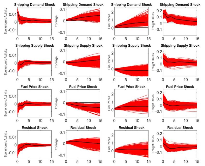
states on the five endogenous variables which become negligible for stationary processes as → ∞.

3.4 Estimation and Inference
 We rely on Bayesian methods of inference, the most common approach in the literature on sign-
identified VAR models.6 We assume a conventional Gaussian-inverse Wishart prior on the reduced-form
parameters and an independent uniform prior on the rotation matrices. Given the vector of reduced-
form parameters, this allows us to generate a large number of candidate solutions for the structural
impact matrix 0−1 based on 5,000 draws from the reduced-form posterior with 20,000 draws of the
rotation matrix each. To do so, we follow Rubio-Ramirez, Waggoner, and Zha (2010) and implement a
QR decomposition using the Householder transformation to generate matrices with orthogonal shocks.
For each candidate solution of the structural impact matrix 0−1 , we compute the set of implied
structural impulse responses. If these impulse responses fulfill the sign restrictions, we retain the
respective structural model.
 To evaluate the posterior of the structural impulse responses, we follow the procedure of Inoue
and Kilian (2013, 2019) and compute the mode (that is, the most likely model) and the joint credible sets
of the admissible structural models. These sets account for the dependence of the elements of the
structural impulses across the admissible models.

4. Results
4.1 Impulse Response Functions
 Figure 6 presents the estimated set of impulse response functions for the four endogenous
variables. The functions show how (from left to right) the percentage change in global economic activity,
the percentage change in world mercantile gross tonnage, the log of the real fuel price index, and the
log of the real dry bulk index react to a one-standard deviation change in (from top to bottom) the
shipping demand shock, the shipping supply shock, the fuel price shock, and the residual shock through
time. The mode and the joint credible sets of the admissible structural models are depicted in black and
red, respectively.
 In the main, the impulse response functions demonstrate that the reaction of real dry bulk
freight rates to the different types of shocks are either in line with what one would reasonably expect or

6
 For more details on Bayesian estimation of sign-identified VAR models, see Kilian and Lütkepohl (2017).
 14

– in effect – indistinguishable from zero. A positive shipping demand shock and a positive fuel price
shock both increase real dry bulk freight rates, but with the former leading to stronger and more long-
lasting effects than the latter. Likewise, a negative shipping supply shock increases real dry bulk freight
rates while a residual shock does not have a clear effect on freight rates. On average, shipping demand
shocks are, by far, the most persistent with their effects lingering up to 10 to 15 years. This is followed
by fuel price shocks and shipping supply shocks which are significantly less persistent with effects that
only last for a few years. Finally, the effect of residual shocks is, for the most part, fairly minimal.

4.2 Historical Decompositions
 Historical decompositions show the contribution of each shock in driving variation in the real dry
bulk freight rate series. They quantify the independent contribution of the four shocks to deviations in
real dry bulk freight rates from their base projection. Figure 7 allows us to visually discern the historical
drivers of booms and busts in the dry bulk shipping industry. The vertical scales are identical across the
four sub-panels so that the figures clearly illustrate the relative importance of a given shock. Another
way of intuitively thinking about these historical decompositions is that each of the sub-panels
represents a counterfactual simulation of what real dry bulk freights rates would have been if it had only
been driven by this particular shock.
 For instance, we can consider the case of shipping demand shocks by integrating the lessons of
economic and financial history on variation in global output. The historical decomposition starts in 1880
when dry bulk freight rates were likely somewhat depressed due to the negative accumulated effects of
shipping demand shocks during the Long Depression of the 1870s. Afterwards, the effects of shipping
demand shocks are in line with our historical knowledge about the business cycles in major economies
at the time. For example, the effects of the large negative shipping demand shock in the late 1900s can
be associated with the Panic of 1907. Likewise, real dry bulk freight rates plummeted in the early 1930s
as the Great Depression dramatically reduced global trade and the demand for shipping services.
 After World War II, positive shipping demand shocks led to increases in real dry bulk freight
rates in the wake of the immediate post-war efforts at re-industrialization and re-urbanization in much
of Europe and Japan as well as the later economic transformation of the East Asian Tigers and Japan.
From 1950 to 1980, this amounted to a nearly uninterrupted — but far from constant — string of
positive shipping demand shocks. This long swing was reversed in the period from 1980 to 2000.
However, from the early 2000s, a series of positive commodity demand shocks emerged which were
clearly related to unexpectedly strong global growth driven by the industrialization and urbanization of
 15

China. Indeed, this period represents the most dramatic upswing in the cumulative effects of shipping
demand shocks seen in these 140 years of global macroeconomic history. The lingering effects of the
Global Financial Crisis are also clearly visible in the series for the accumulated effects of shipping
demand shocks. Finally, the historical decomposition shows that shipping supply shocks, fuel price
shocks, and residual shocks alike had much less of an important role in driving deviations in long-run real
dry bulk freight rates from their underlying trend.
 Table 3 more precisely quantifies these impressions by numerically summarizing the
contribution of each shock by period. For the full period from 1879 to 2020, shipping demand shocks
explain 45% of the variation in real dry bulk freight rates while shipping supply shocks explain 22%.
These two types of fundamental shocks which are related to simple supply and demand conditions,
thus, explain a significant majority (67%) of the medium- and long-run variation in real dry bulk freight
rates. Fuel price shocks and residual shocks respectively explain 11% and 22% of the same.
 It is also possible to replicate this decomposition for shorter spans of time by using the
parameter estimates derived from the full sample in combination with the respective size of shocks for
various sub-periods. In the lower half of Table 3, we consider the independent contribution of the four
shocks in the pre-World War I era from 1880 to 1913, the interwar years from 1919 to 1939, and the
post-World War II era from 1949 to 2020. In the pre-World War I era, we find a more balanced
contribution across shipping demand shocks and shipping supply shocks with shares of 34% and 30%,
respectively. We also find that the contribution of shipping demand shocks to variation in real dry bulk
freight rates increased substantially to 52% in the interwar years while the contribution of shipping
supply shocks decreased substantially to 19% in the same. What is more, the share of shipping demand
shocks remains elevated at 47% and the share of shipping supply shocks remains suppressed at 20% in
the post-World War II era. While there may be several potential explanations for this phenomenon (see
below), we must leave their exploration for future research. In contrast, the contribution of both fuel
price shocks and residual shocks remained roughly constant through the three sub-periods, not straying
very far from the headline numbers of 11% and 22% reported above.

4.3 Sensitivity analysis
 Our results are relatively robust to a number of different approaches to the data. First, we have
previously noted that the use of real global GDP may not be ideal, given changes in the composition of
GDP over time away from goods production and towards services. To this end, we substitute the series
of real global GDP with the series of US industrial production depicted in Panel B of Figure 3. And while
 16

the pairwise correlation for changes in world real GDP and US industrial production from 1850 to 2020 is
0.95, we may also reasonably expect some changes in the values of parameter estimates from the
structural VAR. Likewise, we also substitute the series of real global GDP with the proxy for world
industrial production which covers the OECD plus Brazil, China, India, Indonesia, Russia, and South Africa
and which is depicted in Panel C of Figure 3. Finally, we substitute the series of real fuel prices inclusive
of sail tonnage with an index of real fuel prices which excludes sail tonnage and which is depicted in
Panel C of Figure 4.
 Rather than display and try to visually compare the associated impulse response functions and
historical decompositions, we instead reproduce the decomposition exercise in Table 3 and numerically
summarizing the contribution of each shock by period across the three alternate specifications. The first
panel of Table 4 reports the shares for our benchmark specification. This is then followed by the shares
from the specification using the index of US industrial production, the specification using the index of
OECD +6 industrial production, and finally the specification using the real fuel price index which excludes
sail tonnage.
 There, we find that relative to the benchmark specification, the substitution of the index of US
industrial production for real global GDP leads to a 11 percentage point reduction in the share of
shipping demand shocks from 1880 to 2020. 10 percentage points of this reduction are then evenly split
in between increases in the share of shipping supply shocks and fuel price shocks. However, shipping
demand shocks retain pride of place, both here in the full sample and for two of the three sub-periods.
On balance, we find these results somewhat reassuring, but it is an open question how much
interpretative weight to place on these figures, given the geographic specificity of this proxy for global
economic activity and the waning US share of world industrial production.
 More reassuringly, the substitution of the index of OECD+6 industrial production for real global
GDP delivers results which are numerically more consistent with those for the benchmark specification
in the post-World War II period. Thus, the share of shipping demand shocks only decreases by 5
percentage points while the share of shipping supply shocks remains roughly constant. However, the
largest changes occur: (1) for fuel price shocks which are now reckoned to explain 25% of the variation
in real dry bulk freight rates (a result which is perhaps not surprising given the size of these shocks in the
past 60 years); and (2) for residual shocks which are now reckoned to explain a mere 13% of the same (a
figure which also represents the lowest share of the residual across all specifications and sub-periods).
 Finally, the substitution of the real fuel price index derived without sail tonnage for the real fuel
price index derived with sail tonnage yet again sees shipping demand shocks prevail in the full sample
 17

and for two of the three sub-periods. In sum, these results suggest that while numerical values change
across specifications, the relative ordering of the importance of these shocks remain relatively invariant:
shipping demand shocks are generally the most important driver of booms/busts in the dry bulk
shipping industry followed, in order, by shipping supply shocks, residual shocks, and fuel price shocks.

5. Conclusion
 This paper is the first to provide evidence on the drivers of real maritime transport costs in the
very long-run. To this end, we develop and analyze a new and large dataset on dry bulk freight rates for
the period from 1850 to 2020, finding that, in real terms, these followed a downward, but undulating
path with a cumulative decline of 79% between 1850 and 2020. We relate this secular decline to a
historical literature which documents significant productivity growth as radical changes in goods
handling and storage in ports, naval architecture, and propulsion took place (Harley, 1988; Mohammed
and Williamson, 2004; Tenold, 2019).
 Our next step came in understanding the drivers of booms and busts in the dry bulk shipping
industry. Here, we speak to both a recent academic literature and a long-standing professional
consensus which emphasize the role of shipping demand in governing cyclic patterns of investment and
profitability in the dry bulk industry. Somewhat reassuringly, we find that shipping demand shocks do
indeed strongly dominate all other shocks as a driver of real dry bulk freight rates over the long run.
Furthermore, while shipping demand shocks have increased in importance over time, shipping supply
shocks in particular have become less relevant.
 What remains as tasks for the future comes in developing disaggregated measures of maritime
transport costs across commodity classifications and destination/origin pairings. That is, it would be
useful to have a characterization of the respective shares of shocks for particular commodity-
destination-origin combinations which could then be matched with known features of commodity and
industrial production and their geographical determinants. An additional way forward would also come
in developing a much more refined measure of shipping supply, specifically as it relates to the dry bulk
sector. Here, we have had to abstract away from the implications of increasing specialization by ship
type, technological change in propulsion, and time-varying utilization rates which may vitally affect any
measure of the effective – as opposed to the observed – supply of dry bulk shipping services. Thus, in
any final reckoning of the respective role of fundamentals in the dry bulk shipping market, shipping
supply may yet reemerge as a more dominant force if our current measure of mercantile gross tonnage
diverges too far from actual conditions in the industry.
 18

19

References
Angier, E.A.V. (1920), Fifty Years’ Freights 1869-1919. London: Fairplay.
Baumeister, C. and J.D. Hamilton (2019), “Structural Interpretation of Vector Autoregressions
 with Incomplete Identification: Revisiting the Role of Oil Supply and Demand Shocks.” American
 Economic Review 109(5): 1873-1910.
Baumeister, C., D. Korobilis, and T.K. Lee (2020), “Energy Markets and Global Economic
 Conditions.” CEPR Working Paper 14580.
Beaver, S.H. (1967), “Ships and Shipping: The Geographical Consequences of Technological
 Progress.” Geography 52(2): 133-156.
Brancaccio, G. Kalouptsidi, M. and T. Papageorgiou (2020), “Geography, Transportation, and
 Endogenous Trade Costs.” Econometrica 88(2): 657-691.
Canova, F. and G. De Nicolo (2002), “Monetary Disturbances Matter for Business Fluctuations
 in the G7.” Journal of Monetary Economics 49(6): 1131-1159.
Cufley, C. (1972), Ocean Freights and Chartering. London: Staples Press.
Faust, J. (1998), “The Robustness of Identified VAR Conclusions about Money.” Carnegie-
 Rochester Conference Series on Public Policy 49: 207-244
Greenwood, R. and S.G. Hanson (2015), “Waves in Ship Prices and Investment.” Quarterly
 Journal of Economics 130(1): 55–109.
Hamilton, J.D. (2019), “Measuring Global Economic Activity.” NBER Working Paper 25778.
Harley, C.K. (1988), “Ocean Freight Rates and Productivity, 1740-1913: The Primacy of
 Mechanical Invention Reaffirmed.” Journal of Economic History 48(4): 851-876.
Inoue, A. and L. Kilian (2013), “Inference on Impulse Response Functions in Structural VAR
 Models.” Journal of Econometrics 177(1): 1-13.
Inoue, A. and L. Kilian (2019), “Corrigendum to “Inference on Impulse Response Functions in
 Structural VAR Models.” Journal of Econometrics 209(1): 139-143(1)
Isserlis, L. (1938), “Tramp Shipping Cargoes and Freights.” Journal of the Royal Statistical
 Society 101(1): 53-146.
Jacks, D.S. (2019), “From Boom to Bust: A Typology of Real Commodity Prices in the Long
 Run.” Cliometrica 13(2): 201-220.
Jacks, D.S. and M. Stuermer (2020), “What Drives Commodity Price Booms and Busts?”
 Energy Economics 85: Article 104035.
Jacks, D.S. and J.P. Tang (2018), “Trade and Immigration, 1870-2010.” NBER Working Paper
 25010.
Kalouptsidi, M. (2014), “Time to Build and Fluctuations in Bulk Shipping.” American Economic
 Review 104(2): 564-608.
Kellou, A. (2020), “Low Sulfur Regulations: The Impact on Maritime Shipping Prices.”
 https://market-insights.upply.com/en/low-sulfur-regulations-the-impact-on-maritime-shipping-
 prices
Kilian, L. (2009), “Not All Oil Price Shocks are Alike: Disentangling Demand and Supply
 Shocks in the Crude Oil Market.” American Economic Review 99(3): 1053–69.
Kilian, L. and H. Lütkepohl (2017), Structural Vector Autoregressive Analysis. Cambridge:
 Cambridge University Press.
Kilian, L. and D.P. Murphy (2012), “Why Agnostic Sign Restrictions are Not Enough:
 Understanding the Dynamics of Oil Market VAR Models.” Journal of the European
 Economic Association 10(5): 1166-1188.
Kilian, L. and D.P. Murphy (2014), “The Role of Inventories and Speculative Trading in the
 Global Market for Crude Oil.” Journal of Applied Econometrics 29(3): 454-78.
Kilian, L., N. Nomikos, and X. Zhou (2020), “A Quantitative Model of the Oil Tanker Market in
 20

the Arabian Gulf.” CEPR Discussion Paper 14798.
Kilian, L. and X. Zhou (2018), “Modeling Fluctuations in the Global Demand for
 Commodities.” Journal of International Money and Finance 88: 54-78.
Klovland, J.T. (2009), “New Evidence on the Fluctuations in Ocean Freight Rates in the
 1850s.” Explorations in Economic History 46(3): 266-284.
Klovland, J.T. (2017), “Navigating through Torpedo Attacks and Enemy Raiders: Merchant
 Shipping and Freight Rates during World War I.” NHH Department of Economics Discussion
 Paper 07/2017.
Lundgren, N.-G. (1996), “Bulk Trade and Maritime Transport Costs: The Evolution of Global
 Markets.” Resources Policy 22(1/2): 5-32
Lütkepohl, H. and M. Krätzig (2004), Applied Time Series Econometrics. Cambridge:
 Cambridge University Press.
Maddison, A. (2010), Historical Statistics of the World Economy: 1–2008 AD.
 http://www.ggdc.net/maddison/
Metaxas, B. (1971), The Economics of Tramp Shipping. London: Athlone Press.
Mohammed, S.I.S. and J.G. Williamson (2004), “Freight Rates and Productivity Gains in
 British Tramp Shipping 1869-1950.” Explorations in Economic History 41(2): 172-203.
O’Rourke, K.H. and J.G. Williamson (1994), “Late Nineteenth-Century Anglo-American Factor-
 Price Convergence” Journal of Economic History 54(4): 892-916.
O’Rourke, K.H. and J.G. Williamson (1999), Globalization and History. Cambridge: MIT Press.
Rubio-Ramirez, J.F., D.F. Waggoner, and T. Zha (2010), “Structural Vector Autoregressions:
 Theory of Identification and Algorithms for Inference.” Review of Economic Studies 77(2): 665-
 696.
Sollohub, W.A. (1932), “The Plight of Foreign Trade.” American Economic Review 22(3): 403–
 413.
Stopford, M. (2009), Maritime Economics. New York: Routledge Press.
Stuermer, M. (2018), “150 Years of Boom and Bust: What Drives Mineral Commodity Prices?”
 Macroeconomic Dynamics 22(3): 702-717.
Sturmey, S.G. (1962), British Shipping and World Competition. London: Athlone Press.
Tenold, S. (2019), Norwegian Shipping in the 20th Century. London: Palgrave Macmillan.
Uhlig, H. (2005), “What are the Effects of Monetary Policy on Output? Results from an
 Agnostic Identification Procedure.” Journal of Monetary Economics 52(2): 381-419.
Wegerich, A. (2016), Digging Deeper: Global Coal Prices and Industrial Growth, 1840-1960.
 Ph.D. thesis, Brasenose College, University of Oxford.
UNCTAD (2015), Review of Maritime Transport. Geneva: United Nations Conference on Trade
 and Development.

Appendix A

This appendix details the sources of global economic activity, real fuel prices, real maritime freight rates,
and world mercantile gross tonnage used throughout this paper.

Global economic activity

In the paper, we consider three measures of global economic activity depicted in Panels A through C of
Figure 3. Our benchmark measure is world GDP derived from Maddison (2010) with updates from
Stuermer (2018).

 21

Our second measure is an index of US industrial production for the period from 1850 to 2020 formed by
chaining Davis’ (2004) annual USIP index, Miron and Romer’s (1990) monthly USIP index, and the
Federal Reserve Economic Data’s (2020) non-seasonally adjusted monthly USIP index. The sources are as
follows:

Davis, J.H. (2004), “An Annual Index of US Industrial Production, 1790-1915.” Quarterly
 Journal of Economics 119(4), 1177-1215.
Federal Reserve Economic Data (2020), IPB50001N, Industrial Production: Total Index, Not
 Seasonally Adjusted; https://fred.stlouisfed.org/series/IPB50001N
Miron, J.A. and C.D. Romer (1990), “A New Monthly Index of Industrial Production, 1884-
 1940.” Journal of Economic History 50(2), 321-337.

Finally, for the period, from 1958 to 2020, we also consider an index of world industrial production
which covers the OECD plus Brazil, China, India, Indonesia, Russia, and South Africa. This series was
originally published by the OECD in its Main Economic Indicators database. However, the organization
discontinued the series in 2011. Baumeister and Hamilton (2019) have extended and updated the OECD
series based on the same methodology.

Real fuel prices

The share of world mercantile gross tonnage by fuel type from 1879 depicted in Panel A of Figure 4 were
derived from the world fleet statistics website administered by the Lloyd's Register Foundation:
https://hec.lrfoundation.org.uk/archive-library/world-fleet-statistics

The real fuel price indices depicted in Panels B and C of Figure 4 were then constructed off the shares
above and the real price of petroleum taken from Jacks (2019) and of Welsh best steam coal taken from
Wegerich (2016) with extensions from 1962 using the real price of coal taken from Jacks (2019).

Real maritime freight rates

Freight rates quoted in Great British pounds were converted into real 1990 GBP using the CPI deflator in
O’Donoghue, Goulding, and Allen (2004) with updates from the Bank of England. Freight rates quoted in
US dollars were converted into real 1990 USD using the CPI deflator in Officer and Williamson (2020)
with updates from the Bureau of Labor Statistics.

O’Donoghue, J., L. Goulding, and G. Allen (2004), “Consumer Price Inflation since 1750.”
 Economic Trends 604: 38-46.
Officer, L.H. and S.H. Williamson (2020), "The Annual Consumer Price Index for the United
 States, 1774-Present." http://www.measuringworth.com/uscpi/

The underlying sources for the nominal freight rate data are as follows:

Andrews, F. (1907), “Ocean Freight Rates and the Conditions Affecting Them.” USDA Bureau
 of Statistics Bulletin no. 67. Washington: GPO.
Angier, E.A.V. (1920), Fifty Years’ Freights 1869-1919. London: Fairplay.
Baumeister, C., D. Korobilis, and T.K. Lee (2020), “Energy Markets and Global Economic
 Conditions.” CEPR Working Paper 14580.
Brentano, L. (1911), Die Deutschen Getreidezoelle. Stuttgart.
 22