Model-Based 3D Hand Pose Estimation from Monocular Video
←
→
Page content transcription
If your browser does not render page correctly, please read the page content below
1

     Model-Based 3D Hand Pose Estimation from
                 Monocular Video
    Martin de La Gorce, Member, IEEE, David J. Fleet, Senior, IEEE and Nikos Paragios, Senior, IEEE

                                                                              F

Abstract—A novel model-based approach to 3D hand tracking from
monocular video is presented. The 3D hand pose, the hand texture
and the illuminant are dynamically estimated through minimization of
an objective function. Derived from an inverse problem formulation, the
objective function enables explicit use of temporal texture continuity
and shading information, while handling important self-occlusions and
time-varying illumination. The minimization is done efficiently using a
quasi-Newton method, for which we provide a rigorous derivation of
the objective function gradient. Particular attention is given to terms
related to the change of visibility near self-occlusion boundaries that are
neglected in existing formulations. To this end we introduce new occlu-
sion forces and show that using all gradient terms greatly improves the
performance of the method. Qualitative and quantitative experimental
                                                                                  Fig. 1. Two hand pictures in the first column and their
results demonstrate the potential of the approach.                                corresponding edge map and segmented silhouette in
                                                                                  the two other columns. Edge and Silhouette are little
Index Terms—Hand Tracking, Model Based Shape from Shading, Gen-                   informative to disambiguate the two different index poses.
erative Modeling, Pose Estimation, Variational Formulation, Gradient
Descent
                                                                                  texture and are often self-occluding. Edge information
                                                                                  is often ambiguous due to clutter. For example, the
1    I NTRODUCTION                                                                first column in Fig. 1 shows images of a hand with
Hand gestures provide a rich form of nonverbal human                              different poses of its index finger. The other columns
communication for man-machine interaction. To this                                show corresponding edge maps and silhouettes, which
end, hand tracking and gesture recognition are central                            remain unchanged as the finger moves; as such, they do
enabling technologies. Data gloves are commonly used                              not reliably constrain the hand pose. For objects like the
as input devices but they are expensive and often inhibit                         hand, which are relatively uniform in color, we posit that
free movement. As an alternative, vision-based tracking                           shading is a crucial visual cue. Nevertheless, shading has
is an attractive, non-intrusive approach.                                         not been used widely for articulated tracking (but see [1],
   Fast, effective, vision-based hand pose tracking is,                           [2]). The main reason is that shading constraints require
however, challenging. The hand has approximately 30                               an accurate model of surface shape. Simple models of
degrees of freedom, so the state space of possible hand                           hand geometry where hands are approximated as a small
poses is large. Seaching for the pose that is maximally                           number of ellipsoidal or cylindrical solids may not be
consistent with an image is computationally demanding.                            detailed enough to obtain useful shading constraints.
One way to improve state space search in tracking is to                           Surface occlusions also complicate shading cues.
exploit predictions from recently estimated poses, but                               Two complementary approaches have been suggested
this is often ineffective for hands as they can move                              for monocular hand tracking. Discriminative methods
quickly and in complex ways. Thus, predictions have                               aim to recover hand pose from a single frame through
large variances. The monocular tracking problem is ex-                            classification or regression techniques (e.g., [3], [4], [5],
acerbated by inherent depth uncertainties and reflection                          [6]). The classifier is learned from training data that is
ambiguities that produce multiple local optima.                                   generated off-line with a synthetic model, or acquired by
   Another challenge concerns the availability of use-                            a camera from a small set of known poses. Due to the
ful visual cues. Hands are usually skin colored and it                            large number of hand DOFs it is impractical to densely
is difficult to discriminate one part of the hand from                            sample the entire state space. As a consequence, these
another based solely on color. The silhouette of the                              methods are perhaps best suited for rough initialization
hand, if available, provides only weak information about                          or recognition of a limited set of predefined poses.
the relative positions of different fingers. Optical flow                            Generative methods use a 3D articulated hand model
estimates are not reliable as hands have little surface                           whose projection is aligned with the observed image for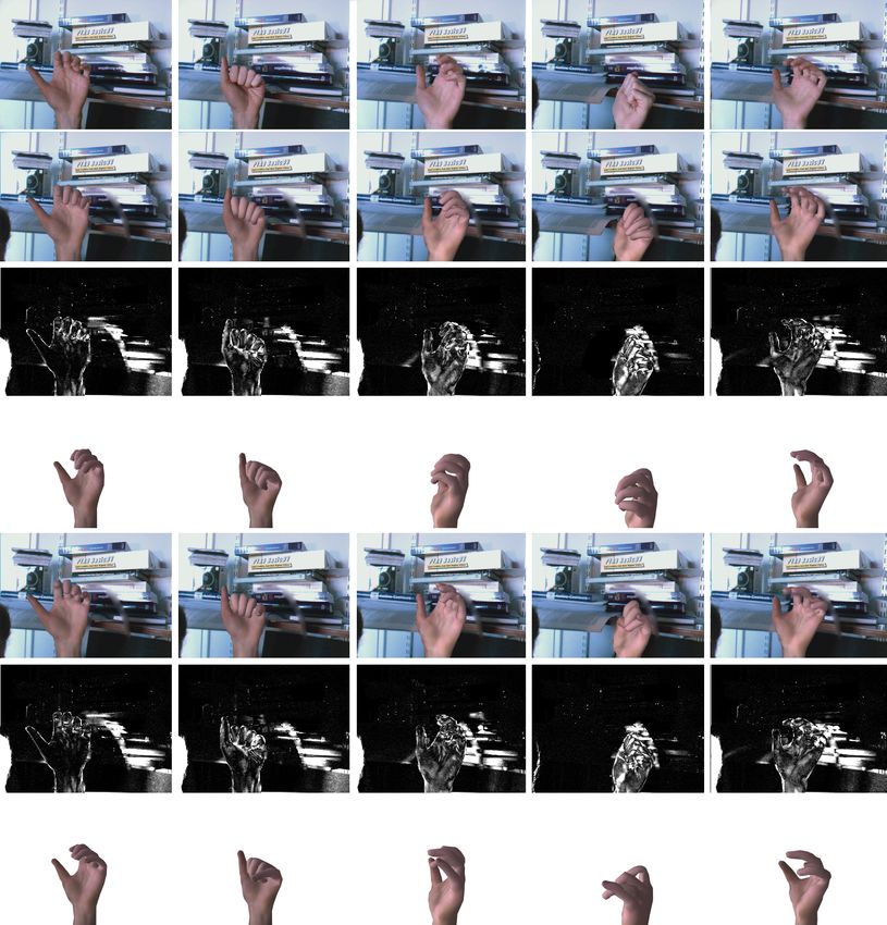
2

pose recovery (e.g., [7], [8], [9], [10], [11]). The model
projection is synthesized on-line and the registration of
the model to the image can be done using local search,
ideally with continuous optimization. A variety of cues
such as the distance to edges, segmented silhouettes
[12], [13] or optical flow [1] can be used to guide the
registration. The method in [14] combines discriminative
and generative approaches but does not use on-line syn-
thesis. A set of possible poses in generated in advance,
which restrict the set of pose that can be tracked.
   Not surprisingly, similar challenges exist for the re-
lated problem of fully-body human pose tracking. For
full-body tracking it is particularly difficult to formulate
good likelihood models due to the significant variability                    (a)                          (b)
in shape and appearance (e.g., see [15]). Interestingly,       Fig. 2. (a) The skeleton (b) The deformed hand triangu-
with the exception of recent work in [16] on human body        lated surface
shape and pose estimation for unclothed people, shading
has not been used extensively for human pose tracking.
  This paper advocates the use of richer generative            2     G ENERATIVE M ODEL
models of the hand, both in terms of geometry and              2.1   Synthesis
appearance, along with carefully formulated gradient-          Our analysis-by-synthesis approach requires an image
based optimization. We introduce a new analysis-by-            formation model, given a 3D hand pose, surface texture,
synthesis formulation of the hand tracking problem that        and an illuminant. The model is derived from well-
incorporates both shading and texture information while        known computer animation and graphics concepts.
handling self-occlusion. Given a parametric hand model,           Following [17], we model the hand surface by a 3D,
and a well-defined image formation process, we seek            closed and orientable, triangulated surface. The surface
the hand pose parameters which produce the synthetic           mesh comprising 1000 facets (Fig. 2b). It is deformed
image that is as similar as possible to the observed           according to pose changes of an underlying articulated
image. Our similarity measure (i.e., our objective function)   skeleton using Skeleton Subspace Deformation [18], [19].
simply comprises the sum of residual errors, taken over        The skeleton comprises 18 bones with 22 degrees of
the image domain. The use of a triangulated mesh-              freedom (DOF). Each DOF corresponds to an articulation
based model allows for a good shading model. By also           angle whose range is bounded to avoid unrealistic poses.
modeling the texture of the hand, we obtain a method           The pose is represented by a vector θ, comprising 22
that naturally captures the key visual cues without the        articulation parameters plus 3 translational parameters
need to add new ad-hoc terms to the objective function.        and a quaternion to define the global position and
   During the tracking process we determine, for each          orientation of the wrist with respect to the camera. To
frame, the hand and illumination parameters by mini-           accommodate different hand shapes and sizes, we also
mizing an objective function. The hand texture is then         add 54 scaling parameters (3 per bone), called morpho-
updated in each frame, and then remains static while           logical parameters. These parameters are estimated during
fitting the model pose and illumination in the next            the calibration process (see Sec. 4.1), subject to linear
frame. In contrast to the approach described in [1],           constraints that restrict the relative lengths of the parts
which relies on optical flow, our objective function does      within each finger.
not assume small inter-frame displacements in its for-            Since hands have relatively little texture, shading is
mulation. It therefore allows large displacements and          essential to modeling hand appearance. Here adopt the
discontinuities. The optimal hand pose is determined           Gouraud shading model and assume Lambertian re-
through a quasi-Newton descent using the gradient of           flectance. We also include an adaptive albedo function to
the objective function. In particular, we provide a novel,     model texture and miscellaneous, otherwise unmodeled,
detailed derivation of the gradient in the vicinity of         appearance properties. The illuminant model includes
depth discontinuities, showing that there are important        ambient light and a distant point source, and is specified
terms in the gradient due to occlusions. This analysis of      by a 4D vector denoted by L, comprising three elements
continuity in the vicinity of occlusion boundaries is also     for a directional component, and one for an ambient
relevant, but yet unexplored, for the estimation of full-      component. The irradiance at each vertex of the surface
body human pose in 3D. Finally, we test our method on          mesh is obtained by the sum of the ambient coefficient
challenging sequences involving large self-occlusion and       and the scalar product between the surface normal at
out-of-plane rotations. We also introduce sequences with       the vertex and the light source direction. The irradiance
3D ground truth to allow for quantitative performance          across each face is then obtained through bilinear inter-
analysis.                                                      polation. Multiplying the reflectance and the irradiance
3

                                                                          Texture T
yields the appearance for points on the surface.                  0   1    2   3   4       6             first patch
                                                                                       5
   Texture (albedo variation) can be handled in two ways.                                      j
                                                              0
                                                                                                         second patch
The first associates an RGB triplet with each vertex of the   1
surface mesh, from which one can linearly interpolate         2
                                                                                                         unused texels

over mesh facets. This approach is conceptually simple        3                                    consistency along edges for integer coordinates
but computationally inefficient as it requires many small
                                                              i                                    T3,0 = T3,3 ; T2,1 = T3,4 ; T1,2 = T3,5 ; T0,3 = T3,6
facets to accurately model smooth surface radiance. The
second approach, widely used in computer graphics,                                                 linearity of the interpolation along diagonal edge
involves mapping an RGB reflectance (texture) image                                                T2,0 + T3,1 = T3,0 + T2,1
onto the surface. This technique preserves detail with                                             T1,1 + T2,2 = T2,1 + T1,2
a reasonably small number of faces.                                   3D mesh                      T0,2 + T1,3 = T1,2 + T0,3
   In contrast with previous methods in computer vision
that used textured models (e.g., [20]), our formulation       Fig. 3. Adjacent facets of the triangulated surface mesh
(Sec. 3) requires that surface reflectance be continuous      project to two triangles in the 2D texture map T . Since
over the surface. Using bilinear interpolation of the dis-    the shared edge projects to distinct segments in the
cretized texture we ensure continuity of the reflectance      texture map, one must specify constraints that the texture
within each face. However, since the hand is a closed         elements along the shared edge be consistent. This is
surface it is impossible to define a continuous bijective     done here using 7 linear equality constraints.
mapping between the whole surface and a 2D planar
surface. Hence, there is no simple way to ensure conti-
nuity of the texture over the entire surface of the hand.     in the texture map. Using bilinear texture mapping, the
   Following [21] and [22], we use patch-based texture        texture intensities of points with non-integer coordinates
mapping. Each facet is associated with a triangular region    (i + 1 − λ, j + λ), λ ∈ (0, 1) along the edge are given by
in the texture map. The triangles are uniform in size
and have integer vertex coordinates. As depicted in               λ(1 − λ)(Ti,j + Ti+1,j+1 ) + λ2 Ti,j+1 + (1 − λ)2 Ti+1,j . (1)
Fig. 3, each facet with an odd (respectively even) index
                                                              By twice differentiating this expression with respect to
is mapped onto a triangle that is the left-upper-half
                                                              λ, we find that it is linear with respect to λ if and only
(respectively right-lower-half) of a square divided along
                                                              if the following linear constraint is satisfied:
its diagonal. Because we use bilinear interpolation we
need to reserve some texture pixels (texels) outside the                           Ti,j + Ti+1,j+1 = Ti+1,j + Ti,j+1 .                              (2)
diagonal edges for points with non-integer coordinates
(see Fig.3). This representation is therefore redundant for   The second set of constraints are for those points along
points along edges of the 3D mesh; i.e., 3D edges of the      the diagonal edges. Finally, let T denote the linear sub-
mesh belong to two adjacent facets and therefore occur        space of valid textures, i.e., whose RGB values satisfy the
twice in the texture map, while each vertex occurs an         linear constraints to ensure continuity over the surface.
average of 6 times (according to the Eulerian properties         Given the mesh geometry, the illuminant, and the
of the mesh). We therefore introduce constraints to en-       texture map, the formation of the model image at each
sure consistency between RGB values at different points       2D image point x can be determined. First, as in ray-
in the texture map that map to the same edge or vertex        tracing, we determine the first intersection between the
of the 3D mesh. By enforcing consistency we also ensure       triangulated surface mesh and the ray starting at the
the continuity of the texture across edges of the mesh.       camera center and passing through x. If no intersection
   With bilinear texture mapping, consistency can be          exists the image at x is determined by the background.
enforced with two sets of linear constraints on the texture   The appearance of each visible intersection point is
map. The first set specifies that the intensities of points   computed using the illuminant and information at the
on mesh edges with integer-coordinates in the texture         vertices of the visible face. In practice, the image is
map must be consistent. The second set enforces the           computed on a discrete grid and the image synthesis
interpolation of the texture to be linear along edges         can be done efficiently using the triangle rasterization
of the triangular patches in the texture map. As long         technique in combination with a depth buffer.
as the texture interpolation is linear along each edge,          When the background is static, we simply assume
and the intensities of the texture map are consistent         that an image of the background is readily available.
at points with integer texture coordinates, the mapping       Otherwise, we assume a probabilistic model for which
will be consistent for all points along each edge. The        background pixel colors are drawn from a background
bilinear interpolation is already linear along vertical and   density pbg (·) (e.g., it can be learned in the first frame
horizontal edges, so we only need to consider the diag-       with some user interaction).
onal edges while defining the second set of constraints.         This completes the definition of the generative process
Let T denote the discrete texture image. Let (i + 1, j)       for hand images. Let Isyn (x; θ, L, T ) denote the synthetic
and (i, j + 1) denote two successive points with integer      image comprising the hand and background, at the point
coordinates along a diagonal edge of a triangular patch       x for a given pose θ, texture T and illuminant L.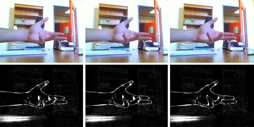
4

                                                                  and about the position of discontinuities in optical flow.
                                                                  Third, (5) is a continuous function of θ; this is not the
                                                                  case for measures based on distances between edges like
                                                                  the symmetric chamfer distance.
                                                                     By changing the domain of integration, the integral of
                                                                  the residual within the hand region can be re-expressed
            Iobs              Isyn               R                as a continuous integral over the visible part of the
                                                                  surface. It can then be approximated by a finite weighted
Fig. 4. The observed image Iobs , the synthetic image Isyn        sum over centers of visible faces. Much of the literature
and the residual image R                                          on 3D deformable models adopts this approach, and as-
                                                                  sumes that the visibility of each face is binary (fully vis-
                                                                  ible or fully hidden), and can be obtained from a depth
2.2   Objective Function                                          buffer (e.g., see [20]). Unfortunately, such discretizations
Our task is to estimate the pose parameters θ, the texture        produce discontinuities in the approximate functional as
T , and the illuminant L that produce the synthesized             θ varies. When the surface moves or deforms, the visibil-
image Isyn () that best matches the observed image,               ity state of a face near an occlusion boundary is likely to
denoted Iobs (). Our objective function is based on a             change, causing a discontinuity in the sum of residuals.
simple discrepancy measure between these two images.              This is problematic for gradient-based optimization. To
First, let the residual image R be defined as                     preserve continuity of the discretized functional with
                                                                 respect to θ, the visibility state should not be binary.
        R(x; θ, T, L) = ρ Isyn (x; θ, L, T ) − Iobs (x) , (3)     Rather, it should be a real-valued and smooth as the
where ρ is either the classical squared-error function            surface becomes occluded or unoccluded. In practice,
or a robust error function such as the Huber function             this is cumbersome to implement and the derivation of
used in [23]. For our experiments we choose ρ to be the           the gradient is complicated. Therefore, in contrast with
conventional squared-error function, and therefore the            much of the literature on 3D deformable models, we
pixel errors are implicitly assumed to be IID Gaussian.           keep the formulation in the continuous image domain
Contrary to this IID assumption, nearby errors often tend         when deriving the expression of functional gradient.
to be highly correlated in practice. This is mainly due to           To estimate the pose θ and the lighting parameters L
simplifications of the model. Nevertheless, as the quality        for each new image frame, or to update the texture T ,
of the generative model improves, as we aim to do in              we look for minima of the objective function. During
this paper, these correlations become less significant.           tracking, the optimization involves two steps. First we
  When the background is defined probabilistically, we            minimize (5) with respect to θ and L, to register the
separate the image domain Ω (a continuous subset of R2 )          model with respect to the new image. Then we minimize
into the region S(θ) covered by hand, given the pose,             the error function with respect to the texture T to find
and the background Ω\S(θ). Then the residual can be               the optimal texture update.
expressed using the background color density as

                   ρ Isyn (x; θ, L, T ) − Iobs (x)), ∀x ∈ S(θ)    3   PARAMETER E STIMATION
R(x; θ, L, T ) =
                   − log pbg (Iobs (x)) , ∀x ∈ Ω\S(θ)             The simultaneous estimation of the pose parameters θ
                                                            (4)
                                                                  and the illuminant L is a challenging non-linear, non-
Fig. 11 (rows 3 and 6) depicts an example of the residual
                                                                  convex, high-dimensional optimization problem. Global
function for the likelihood computed in this way.
                                                                  optimization is impractical and therefore we resort to an
  Our discrepancy measure, E, is defined to be the
                                                                  efficient quasi-Newton, local optimization. This requires
integral of the residual error over the image domain Ω:
                                                                  that we are able to efficiently compute the gradient of E
                            Z
                                                                  in (5) with respect to θ and L.
              E(θ, T, L) =      R(x; θ, L, T ) dx           (5)
                              Ω                                      The gradient of E with respect to lighting L is straight-
                                                                  forward to derive. The synthetic image Isyn () and the
This simple discrepancy measure is preferable to more
                                                                  residual R() are smooth functions of the lighting param-
sophisticated measures that combine heterogeneous cues
                                                                  eters L. As a consequence, we can commute differentia-
like optical flow, silhouettes, or chamfer distances be-
                                                                  tion and integration to obtain
tween detected and synthetic edges. First, it avoids the
                                                                                                 Z
tuning of weights associated with different cues that is                     ∂E                ∂
                                                                                 (θ, L, T ) =       R(x; θ, L, T ) dx
often problematic; in particular, a simple weighted sum                      ∂L               ∂L Ω
                                                                                              Z                            (6)
of errors from different cues implicitly assumes (usually                                        ∂R
incorrectly) that errors in different cues are statistically                                =       (x; θ, L, T ) dx .
                                                                                               Ω ∂L
independent. Second, the measure in (5) avoids early
decisions about the relevance of edges through thresh-            Computing ∂R ∂L (x; θ, L) is straightforward with applica-
olding, about the area of the silhouette by segmentation,         tion of the chain rule to the generative process.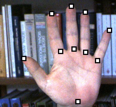
5

                                Γθ
                           x                                      The first term, the partial derivative of E with respect
                                n̂Γθ(x)                           to θ, with β fixed, corresponds to the integration of the
                                                                  residual derivative everywhere except the discontinuity:
                    occlusions boundary Γθ
      Γθ            segment crossing Γθ at x                                            Z
                                                                                 ∂E                ∂r
                    occluding side                                                   =                (x, θ) dx .      (10)
                    near occluded side                                           ∂θ      [0,1]\{β} ∂θ
                   (a)                                (b)
                                                                  The second term in (9) depends on the partial derivative
Fig. 5. (a) Example of a segment crossing the occlusions          of E with respect to the boundary location β. Using the
boundary Γθ . (b) A curve representing the residual along         fundamental theorem of calculus, this term reduces to
this segment                                                      the difference between the residuals at both sides of the
                                                                  occlusion boundary, multiplied by the derivative of the
                                                                  boundary location β with respect to the pose parameters
   Formulating the gradient of E with respect to pose             θ. From (8) it follows that
θ is not straightforward. This is the case along occlu-
sion boundaries where the residual is a discontinuous                        ∂E ∂β                           ∂β
                                                                                   = [r0 (β, θ) − r1 (β, θ)]    .         (11)
function. As a consequence, for this subset of points,                       ∂β ∂θ                           ∂θ
R(x; θ, L, T ) is not differentiable and therefore we cannot      While the residual r(x, θ) is a discontinuous function of
commute differentiation and integration. Nevertheless,            θ at β, the energy E is still a differentiable function of θ.
while the residual is discontinuous, the energy function
remains continuous in θ. The gradient of E with respect           3.1.2 General 2D Case
to θ can therefore be specified analytically. Its derivation      The 2D case is a generalization of the 1D example. Like
is the focus of the next section.                                 the 1D case, the residual image is spatially continuous
                                                                  almost everywhere, except for points at occlusion bound-
3.1    Gradient With Respect to Pose and Lighting                 aries. At such points the hand occludes the background
The generative process above was carefully formulated             or other parts of the hand (see Fig. 5a). Let Γθ be
so that scene radiance is continuous over the hand. We            the set of boundary points, i.e., the support of depth
further assume that the background and the observed               discontinuities in the image domain. Because we are
image are known and continuous. Therefore the residual            working with a triangulated surface mesh, Γθ can be
error is spatially continuous everywhere except at self-          decomposed into a set line segments. More precisely,
occlusion and occlusions boundaries denoted by Γθ .               Γθ is the union of the projections of all visible portions
                                                                  of edges of the triangulated surface that separate front-
3.1.1 1D Illustration                                             facing facets from back-facing facets. For any point x in
                                                                  Γθ , the corresponding edge projection locally separates
To sketch the main idea behind the gradient derivation
                                                                  the image domain into two subregions of Ω\Γθ , namely,
we first consider a 1D residual function on a line segment
                                                                  the occluding side and the near-occluded side (see Fig. 5).
that crosses a self-occlusion boundary, as shown in Fig. 5.
                                                                    Along Γθ , the residual image R() is discontinuous with
Along this line segment the residual function is contin-
                                                                  respect to x and θ. Nevertheless, like in the 1D case, to
uous everywhere except at the self-occlusion location, β.
                                                                  derive ∇E, we need to define a new residual R+ (θ, x),
Accordingly we express the residual on the line in two
                                                                  which extends R() by continuity onto the occluding
parts, namely, the residual to the left of the boundary r0
                                                                  points Γθ . This is done by replicating the content of R()
and the residual on the right r1 :
                                                               in Ω\Γθ from the near-occluded side. In forming R+ , we
                         r0 (x, θ), x ∈ 0, β(θ)                  are recovering the residual of occluded faces in the vicinity
           r(x, θ) =                              .    (7)
                         r1 (x, θ), x ∈ β(θ), 1                   of the boundary points. Given a point x on a boundary
                                                                  segment with outward normal n̂Γθ (x) (i.e., facing the
Accordingly, the energy is then the sum of the integral
                                                                  near-occluded side as in Fig. 5a), we define
of r0 on the left and the integral of r1 on the right:
              Z β(θ)                Z 1                                                                 n̂Γ (x)
                                                                           R+ (θ, x) = lim R θ, x+ θ                 .     (12)
        E =          r0 (x, θ) dx +     r1 (x, θ) dx . (8)                              k→∞                 k
               0                               β(θ)
                                                                  One can interpret R+ (θ, x) on Γθ as the residual we
Note that β is a function of the pose parameter θ.                would have obtained if the near-occluded surface had
Intuitively, when θ varies the integral E is affected in          been visible instead of the occluding surface.
two ways. First the residual functions r0 and r1 vary, e.g.          When a pose parameter θj is changed with an in-
due to shading changes. Second, the boundary location             finitesimal step dθj , the occluding contour Γθ in the
β also moves.                                                     neighborhood of x moves with an infinitesimal step
  Mathematically, the total derivative of E with respect          vj (x) dθj (see (34) for a definition of the boundary speed
to θ is the sum of two terms,                                     vj ). Then the residual in the vicinity of x is discontinu-
                    dE   ∂E   ∂E ∂β                               ous, jumping between R+ (θ, x) and R(θ, x). However, the
                       =    +       .                       (9)
                    dθ   ∂θ   ∂β ∂θ                               surface area where this jump occurs is also infinitesimal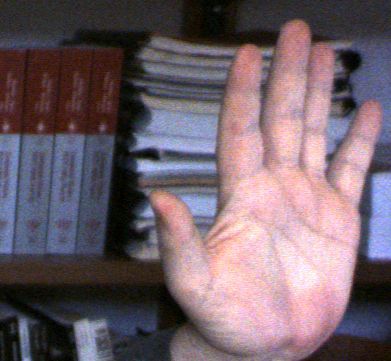
6

and proportional to vj (x) n̂Γθ (x) dθj . The jump causes         ∇˜ θ E 6= ∇θ Ẽ. Most iterative gradient-based optimiza-
an infinitesimal change in E after integration over the           tion methods require direct numerical evaluation of the
image domain Ω.                                                   objective function to ensure that energy decreases at
  Like the 1D case, one can express the functional gra-           each iteration. Such methods expect the gradient to be
                ∂E            ∂E
dient ∇θ E ≡ ( ∂θ 1
                    , . . . , ∂θ n
                                   ) using two terms:             consistent with the objective function.
            Z                                                        Alternatively, one might try to compute the exact
 ∂E               ∂R
       =                 (x; θ, L, T )dx                   (13)   gradient of the approximate objective function, i.e.,
 ∂θj         Ω\Γθ ∂θ   i                                          ∇Ẽ. Unfortunately, due to the aliasing along occluding
        Z
              +                                                 edges (i.e., discretization noise in the sampling in (14)),
      −       R (x; θ, T, L)−R(x; θ, L, T ) n̂Γθ (x) vi (x) dx
          Γθ |                        {z              }           Ẽ(θ, T, L) is not a continuous function of θ. Discontinu-
                              foc (x)                             ities occur, for example, when an occlusion boundary
                                                                  crosses the center of a pixel. As a result of these dis-
The first term captures the energy variation due to the
                                                                  continuities, one cannot compute the exact derivative,
smooth variation of the residual in Ω\Γθ . It integrates
                                                                  and numerical difference approximations are likely to
the partial derivative of the residual R with respect to
                                                                  be erroneous.
θ everywhere but at the occluding contours Γθ , where it
                                                 ∂R
is not defined. The analytical derivation of ∂θ    i
                                                     on Ω\Γθ
requires application of the chain rule to the functions           3.2    Differentiable Discretization of Energy E
that define the generative process.                               To obtain a numerical approximation to E that can be
   The second term in (13) captures the energy variation          differentiated exactly, we consider an approximation to
due to the movement of occluding contours. It integrates          E with antialiasing. This yields a discretization of the
the difference between the residual on either side of             energy, denoted Ē, that is continuous in θ and can be
the occluding contour, multiplied by the normal speed             differentiated in closed form using the chain rule, to
of the boundary when the pose varies. Here, foc is a              obtain ∇θ Ē. The anti-aliasing technique is inspired by
vector field whose directions are normal to the curve             the discontinuity edge overdraw method [28]. We use it
and whose magnitudes are proportional to the difference           here to form a new residual function, denoted R̄.
of the residuals on either each side of the curve. These             The anti-aliasing technique progressively blends the
occlusion forces account for the displacement of occlusion        residuals on both sides of occlusion boundaries. For a
contours as θ varies. They are similar to the forces              point x that is close to an occluding edge segment we
obtained with 2D active regions [24], which derives from          compute a blending weight that is proportional to the
the fact that we kept the image domain Ω continuous               signed distance to the segment:
while computing the functional gradient. Because the
surface is triangulated, Γθ is a set of image line segments,                                  (x − q(x)) · n̂
                                                                                    w(x) =                        ,       (15)
and we could rewrite (13) in a form that is similar to the                                   max(|n̂x |, |n̂y )|)
gradient flow reported in [25] for active polygons. Our
                                                                  where q(x) is a point on the nearby segment, and
occlusion forces also bear similarity to the gradient flows
                                                                  n̂ = (n̂x , n̂y ) is the unit normal to the segment (pointing
of [26], [27] for multi-view reconstruction, where some
                                                                  toward the near-occluded side of the boundary). Dividing
terms account for the change of visibility at occlusion
                                                                  the signed distance by max(|n̂x |, |n̂y |) is a minor conve-
boundaries. In their formulation no shading and texture
                                                                  nience that allows us to interpret terms of the gradient
are attached to the reconstructed surface, which results
                                                                  ∇θ Ē in terms of the occlusion forces defined in (13). A
in substantial differences in the derivation.
                                                                  detailed derivation is given in Appendix A.
3.1.3   Computing ∇θ E                                               Let the image segment V̄m V̄n be defined by end points
                                                                  V̄m and V̄n . For V̄m V̄n we define an anti-aliased region,
A natural numerical approximation to E is to first sam-
                                                                  denoted A, as a set of points on the occluded side near
ple R at discrete pixel locations and then sum, i.e.,
                                                                  the segment (see Fig. 17); i.e., points that that project to
                                X
   E(θ, T, L) ≈ Ẽ(θ, T, L) ≡        R(x; θ, L, T ) . (14)        the segment with weights w(x) in [0, 1);
                                 x∈Ω∩N2
                                                                        A = {x ∈ R2 | w(x) ∈ [0, 1), q(x) ∈ V̄m V̄n } .   (16)
Similarly, one might discretize the two terms of the
gradient ∇θ E in (13). The integral over Ω\Γθ could be            For each point in this region we define the anti-aliased
approximated by a finite sum over image pixel in Ω ∩ N2           residual to be a linear combination of the residuals on
while the integral along contours Γθ could be approxi-            the occluded and occluding sides:
mated by sampling a fixed number of points along each                   R̄(x; θ, L, T ) =w(x)R(x; θ, L, T )
             ˜ θ E be the numerical approximation to the
segment. Let ∇                                                                                                            (17)
                                                                                        + (1 − w(x))R(q(x); θ, L, T ) .
gradient obtained in this way.
  There are, however, several practical problems with             The blending is not symmetric with respect to the line
this approach. First, the approximate gradient is not the         segment, but rather it is shifted toward the occluded
exact gradient of the approximate objective function, i.e.,       side. This allows use of a Z-buffer to handle occlusions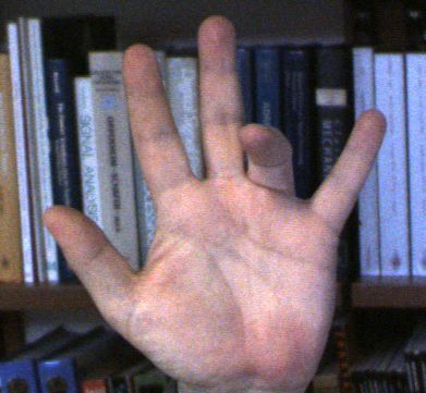
7

(see [28] for details). For all points outside the anti-        [32] with an adapted Broyden-Fletcher-Goldfarb-Shanno
aliased regions we let R̄(x; θ, L, T ) = R(x; θ, L, T ).        (BFGS) Hessian approximation. This allows us to com-
   Using this anti-aliased residual image, R̄, we define a      bine the well-known BFGS quasi-Newton method with
new approximation to the objective function, denoted Ē:        the linear joint limit constraints. There are 4 main steps:
                            X                                     1) A quadratic program is used to determine a de-
            Ē(θ, T, L) =         R̄(x; θ, L, T ) .      (18)         scent direction. This uses the energy gradient and
                           x∈Ω∩N2
                                                                      an approximation to the Hessian, H̃t , based on a
This anti-aliasing technique makes R̄ and thus Ē contin-             modified BFGS procedure (see Appendix B):
uous with respect to θ even along occlusion boundaries.
                                                                                           dĒ            1
  There are other anti-aliasing methods such as over-                  ∆P =       argmin       (Pt )∆P + ∆tP H̃t ∆P (21)
                                                                                           dP             2
sampling [29] or A-buffer [30]. They might reduce the                               ∆P
magnitude of the jump in the residual when an occlusion                    s.t. A(Pt +∆P ) ≤ b
boundary crosses the center of a pixel, as θ changes,
                                                                  2) A line search is then performed in that direction:
perhaps making the jump visually imperceptible, but the
residual remains discontinuous in θ. The edge overdraw                    λ∗ = argmin Ē(Pt + λ∆P ) s.t. λ ≤ 1 .        (22)
method we use in (17) ensures the continuity of R̄ and                              λ
hence Ē with respect to θ.                                          The inequality λ ≤ 1 ensures that we stay in the
  To derive ∇θ Ē we differentiate R̄ using the chain rule.          linearly constrained subspace.
                       X ∂                                        3) The pose and lighting parameters are updated
             ∇θ Ē =            R̄(x; θ, L, T ) .      (19)
                           2
                             ∂θ                                                         Pt+1 = Pt + λ∗ ∆P .             (23)
                        x∈Ω∩N

Using a backward ordering of derivative multiplications            4) The approximate Hessian H̃t+1 is updated using
(called adjoint coding in the algorithm differentiation               the adapted BFGS formula.
literature [31]), we obtain an evaluation of the gradient       These steps are iterated until convergence.
with computational cost that is comparable to the eval-            To initialize the search with a good initial guess, we
uation of the objective function.                               first perform a 1D search along the line that linearly
   The gradient of Ē with respect to θ, i.e., ∇θ Ē, is one    extrapolates the two previous pose estimates. Each local
of the possible discretizations of the analytical ∇θ E. The     minimum obtained during this 1D search is used as a
differentiation of the anti-aliasing process with respect       starting point for our SQP method in the full pose space.
to θ yielded terms that sum along the edges and that            The number of starting points found is usually just one,
can been interpreted as a possible discretization of the        but when there are several, the results of the SQP method
occlusion forces in (13). This is explained in Appendix A.      are compared and the best solution is chosen. Once the
The advantage of this approach over that discussed in           model is fit to a new frame, we then update the texture,
section 3.1.3 is that ∇θ Ē is the exact gradient of Ē, and    which is then used during registration in the next frame.
both can be numerically evaluated. This also allows one
to check validity of the gradient ∇θ Ē obtained by direct
                                                                3.4   Texture Update
comparison with divided differences on Ē. Divided dif-
ferences are prone to numerical error and inefficient, but      Various methods for mapping images onto a static 3D
help to detect errors in the gradient computation.              surface exist. Perhaps the simplest method involves, for
                                                                each 3D surface point, (1) computing its projected image
                                                                coordinates, (2) checking its visibility by comparing its
3.3   Model Registration                                        depth with the depth buffer, and (3) if the point is visible,
3.3.1 Sequential Quadratic Programming                          interpolating image intensities at the image coordinates
During the tracking process, the model of the hand is           and then recovering the albedo by dividing the interpo-
registered to each new frame by minimizing the approx-          lated intensity by the model irradiance at that point. This
imate objective function Ē. Let P = [θ, L]T comprise the       approach is not suitable for our formulation for several
unknown pose and lighting parameters, and assume we             reasons. First, we want to model texture for hidden areas
obtain an initial guess by extrapolating estimates from         of the hand, as they may become visible in the next
the previous frames. We then refine the pose and lighting       frame. Second, our texture update scheme must avoids
estimates by minimizing Ē with respect to P , subject to       progressive contamination by the background color, or
linear constraints which enforce joint limits.                  self-contamination between different parts of the hand.
                                                                   Here, we formulate texture estimation as the mini-
                 P̃ =      argmin Ē(P )                (20)    mization of the same basic objective functional as that
                               P                                used for tracking, in combination with a smoothness
                         s.t. AP ≤ b                            regularization term (independent of pose and lighting).
                                                                That is, for texture T we minimize
   Using the object function gradient, we minimize
Ē(P ) using a sequential quadratic programming method                    Etexture (T ) = Ē(θ, L, T ) + βEsm (T ).     (24)
8

Fig. 6. Observed image and extracted texture mapped
on the hand under the camera viewpoint and two other
viewpoints. The texture is smoothly diffused into regions
that are hidden from the camera viewpoint

                                                            Fig. 7. Estimation of the pose, lighting and morphological
For simplicity the smoothness measure is defined to be      parameters in the frame 1. The first row shows the input
the sum of squared differences between adjacent pixels      image, the synthetic image given rough manual initial-
in the texture (texels). That is,                           ization, and its corresponding residual. The second row
                         X X                                shows the result obtained after convergence
             Esm (T ) =           kTi − Tj k2 ,    (25)
                        i   j∈NT (i)
                                                            4.1   Initialization
where NT (i) represents the neighborhood of the texel i.    A good initial guess for the pose is required for the
While updating the texture, we choose ρ (appearing in       first frame. One could use a discriminative method to
the definition of R and hence R̄ and Ē) to be a trun-      obtain a rough initialization (e.g., [3]). However, as this
cated quadratic instead of the quadratic used for model     is outside the scope of our approach at present, so we
fitting. This helps to avoid the contamination of the       simply assume prior knowledge. In particular, the hand
hand texture by background color whenever the hand          is assumed to be roughly parallel to the image plane at
model fit is not very accurate. The minimization of the     initialization (Fig. 7). We further assume that the hand
function Etexture (T ) with T ∈ T can be done efficiently   color (albedo) is initially constant over the hand surface,
using iteratively reweighed least-squares. The smooth-      so the initial hand appearance is solely a function of pose
ness term effectively diffuses the colour to texels that    and shading. The RGB hand color, along with the hand
do not directly contribute to the image, either because     pose, the morphological parameters, and the illuminant
they are associated to a occluded part (Fig.6) or because   are estimated simultaneously using the quasi-Newton
of texture aliasing artifacts. To improve robustness we     method (see row 2 of Fig. 7 (see the video 1). The
also remove pixels near occlusion boundaries from the       background image or its histogram are also provided
integration domain Ω when computing E(θ, L, T ), and        by the user. Once the morphological parameters are
we bound the difference between the texture in the first    estimated in frame 1, they remain fixed for the rest of
frame and in subsequent texture estimates.                  the sequence.
   Finally, although cast shadows provide useful cues,
they are not explicitly modeled in our approach. In-
stead, they are modeled as texture. Introducing cast        4.2   Finger Bending and Occlusion Forces
shadows in our continuous optimization framework is         In the first sequence (Fig. 8 and video 2) each finger
not straightforward as it would require computation of      bends in sequential order, eventually occluding other
related terms in the functional gradient. Nevertheless,     fingers and the palm. The background image is static,
despite the lack of cast shadows in our model, our          and was obtained from a frame where the hand was not
experiments demonstrate good tracking results.              visible. Each frame has 640 × 480 pixels. Note that the
                                                            edges of the synthetic hand image match the edges in
                                                            the input image, despite the fact that we did not use
4   E XPERIMENTAL R ESULTS                                  any explicit edge-related term in the objective function.
                                                            Misalignment of the edges in the synthetic and observed
We applied our hand pose tracking approach to se-           images creates a large residual in the area between
quences with large amounts of articulation and occlu-       these edges and produces occlusion forces on the hand
sion, and to two sequences used in [14], for comparison     pointing in the direction that reduces the misalignment.
with a state-of-the-art hand tracker. Finally, we also         To illustrate the improvements provided by occlusion
report quantitative results on a synthetic sequence as      forces, we simply remove the occlusion-forces when
well as a real sequence for which ground truth data         computing the energy gradient. The resulting algorithm
were obtained. While the computational requirements         is unable track the hand for any significant period.
depends on image resolution, for 640 × 480 images, our         It is also interesting to compare the minimization of
implementation in C++ and Matlab takes approximately        the energy in (18) with the approach outlined in Sec.
40 seconds per frame on a 2Ghz workstation.                 2.2, which sums errors over the surface of the 3D mesh.
9
Fig. 9. Recovery from failure of the sum-on-surface
method (Sec. 4.2) by our method with occlusion forces.
equal; their difference is bounded by the error induced
by the discretization of integrals. For both methods we
used a maximum of 100 iterations, which was usually
sufficient for convergence.
The alternative approach produces reasonable results
(Fig. 8 rows 5-7) but fails to recover the precise location
of the finger extremities when they bend and occlude
the palm. This is evident in column 3 of Fig. 8 where a
large portion of the little finger is missing. Our approach
(rows 2-4) yields accurate pose estimates through the
entire sequence. The alternative approach fails because
the hand/background silhouette is not particularly infor-
mative about the position of fingertips when fingers are
bending. The residual error is localized near the outside
extremity of the synthesized finger. Self-occlusion forces
are necessary to pull the finger toward this region.
We further validate our approach by choosing the
hand pose estimated by the alternative method (Fig. 8,
column 3, rows 5-7) as an initial state for our tracker with
Fig. 8. Improvement due to self-occlusion forces: Rows 2- occlusion forces (Fig. 9 and video 3). The initial pose and
4 are obtained using our method. Rows 5-7 are obtained the corresponding residual are shown in column 1. The
by summing the residual on the triangulated surface. poses after 25 and 50 iterations are shown in columns 2
Each row shows, from top to bottom: (1) the observed and 3, at which point the pose is properly recovered.
image; (2) the final synthetic image; (3) the final residual
image; (4) a synthetic side view at 45◦ ; (5) the final
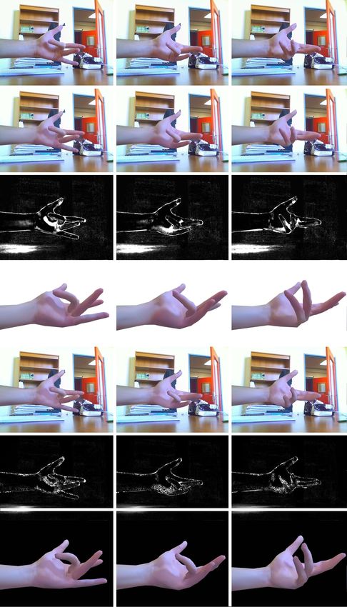
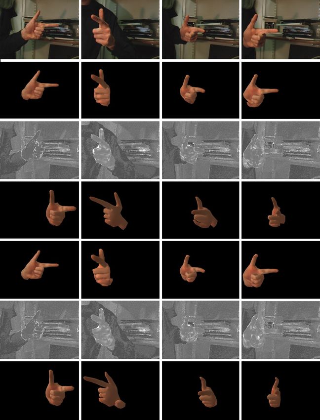
synthetic image with residual summed on surface; (6) 4.3 Stenger Sequences [14]
the residual for visible points on the surface, and (7) the The second and third sequences (Fig. 10, Fig. 11, video
synthetic side view. 4 and 5) were provided by Stenger for direct compar-
ison with their state-of-the-art hand tracker [14]. Both
sequences are 320 × 240 pixels. In Sequence 2 the hand
These 3D points are uniformly distributed on the surface opens and closes while rotating. In Sequence 3 the
and their binary visibility is computed at each step of index finger is pointing while the hand rotates in a
the quasi-Newton process. To account for the change of rigid manner. Both sequences exhibit large inter-frame
summation domain (from image to surface), the error displacements which makes it difficult to predict good
associated to each point is weighted by the inverse of the initial guesses for minimization. The fingers also touch
ratio of surface areas between the 3D triangular face and one another often. This is challenging because our opti-
its projection. The errors associated with the background mization framework does not prohibit the interpenetra-
are also taken into account, to remain consistent with the tion of hand parts. Finally, the background in Sequence
initial cost function. This also prohibits the hand from 3 is dynamic so the energy function has been expressed
receding from the camera so that its projection shrinks. using (4).
We included occlusion forces between the hand and For computational reasons, Stenger et al. [14] used
background to account for variations of the background a form of state-space dimension reduction, adapted to
visibility while computing the energy gradient. The func- each sequence individually (8D for Sequence 2 - 2 for
tional computed in both approaches would ideally be articulation and 6 for global motion - and 6D rigid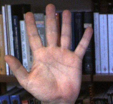
10

Fig. 10. Sequence 2: Each row shows, from top to bot-
tom: (1) the observed image, (2) the final synthetic image
with limited pose space, (3) the final residual image, (4)
the synthetic side view with an angle of 45◦ , (5) the final
synthetic image with full pose space, (6) the residual
image and (7) the synthetic side view.
                                                               Fig. 11. Sequence 3: Each row shows, from top to bot-
                                                               tom: (1) the observed image; (2) the final synthetic image
movement for Sequence 3). We tested our algorithm both         with limited pose space; (3) the final residual image; (4)
with and without pose-space reductions (respectively           the synthetic side view with an angle of 45◦ ; (5) the final
rows 2-4 and 5-7). For pose-space reduction, linear in-        synthetic image with full pose space; and (6) the residual
equalities were defined between pairs or triplet of joint      image, the synthetic side view.
angles. This allowed us to limit the pose space while
keeping enough freedom of pose variation to make fine
registration possible. We did not update the texture for
those sequences after the first frame. With pose-space
reduction our pose estimates are qualitatively similar
to Stenger’s, although smoother through time. Without
pose-space reduction, Stenger’s technique becomes com-
putationally impractical while our approach continues
to produce good results. The lack of need for offline
training and sequence-specific pose-space reduction are
major advantages of our approach.                              Fig. 12. Sequence 4: Two hands. The rows depicts
                                                               4 frames of the sequence, corresponding to (top) the
4.4   Occlusion                                                observed images, (middle) images synthesized using the
Sequence 4 (Fig. 12 and video 6) demonstrates the              estimated parameters, and (bottom) the residual images.
tracking of two hand, with significant occlusions as the
left hand progressively occludes the right. Texture and
pose parameters from both hands are simultaneously             we kept all 28 DOFs on each hand while performing
estimated, and self-occlusions of one hand by another          pose estimation.
are modeled just as was done with a single hand. Fig.
12 shows that the synthetic image looks similar to the
                                                               4.5   Quantitative Performance on Natural Images
observed image, due to the shading and texture models.
In row 2, the ring finger and the little finger of the right   While existing papers on hand pose tracking have relied
hand are still properly registered despite the large occlu-    mainly on qualitative demonstrations for evaluation,
sion. Despite the translational movement of the hands,         here we introduce quantitative measures on a binocular
11
40
90 index tip index MP
middle tip middle MP
35
80 ring tip ring MP
pinky tip pinky MP
70 thumb tip 30 thumb MP
palm basis
60
distance in mm
25
distance in mm
50
20
40
15
30
10
20
5
10
0
50 100 150 200 250 300 350 50 100 150 200 250 300 350
# frame # frame
Fig. 13. Distance between reconstructed and ground
truth 3D locations: (left) The distances for each of the
finger tips; (right) The distances for each of the metacar-
pophalangeal point and the palm basis.
sequence (see video 7) from which we can estimate 3D
ground truth at a number of fiducial points.
The hand was captured with two synchronized, cali-
brated cameras (see rows 1 and 4 in Fig. 14). To obtain
ground truth 3D measurements on the hand, we manu-
ally identified at each frame, the locations of 11 fiducial
points on the hand, i.e., each finger tip, each metacar-
pophalangeal (MP)joint, and the base of the palm. These
locations are shown in the top-left image of Fig. 14. From
these 2D locations in two views we obtain 3D ground Fig. 14. Binocular Video: The columns show frames 2,
truth by triangulation [33]. 220, 254 and 350. Each row, from top to bottom, depicts:
The hand was tracked using just the right image (1) the image from the right camera; (2) the corresponding
sequence. For each of the 11 fiducial points we then synthetic image; (3) the residual for the right view; (4) the
computed the distance between the 3D ground truth observed left image (not used for tracking); and (5) the
and the estimated position on the reconstructed hand synthetic image seen from the left camera.
surface. Because the global size of our model does not
necessarily match the true size of the hand, in each frame
we allow a simple scaling transform of the estimated and cast shadows in the rendering process, neither of
hand to minimize the sum of squared distances between which are explicitly modeled in our tracker. Row 1 of
the 3D ground truth points and the recovered locations. Fig.15 shows several frames from the sequence.
The residual Euclidean errors for each point, after this A quantitative evaluation of estimated pose is obtain
scaling, are shown in Fig. 13. by measuring, for each frame, a distance between the re-
Errors for the thumb tip are large for frames 340-360, constructed 3D surface and the ground truth 3D surface.
and errors for the middle finger are large for frames 240- For visualization of depth errors over the visible portion
350. During those periods the optimization lost track of of the hand surface, we define a distance image Ds :
the positions of the middle finger (see Fig.14 column
3) and the thumb (see Fig.14 column 4). Thumb errors Ds (p) = inf Π−1 Ss (p), q if p ∈ Ωs , ∞ otherwise (26)
q∈Sg
are also large between frames 50 and 150, despite the
fact that estimated pose appears consistent with the where Sg is the ground truth hand surface, Ss is the
right view used for tracking (see residuals in Fig.14 row reconstructed hand surface, and Ωs is the silhouette of
3, columns 1-3). This reflects the intrinsic problem of the surfaces Ss in the image plane. In addition, Π−1 Ss is
monocularly estimating depth. The last row in Fig.14 the back projection function onto the surface Ss ; i.e., the
shows the hand model synthesized from the left camera function that maps each point p in Ωs to the correspond-
viewpoint, for which the depth errors are evident. ing point on the 3D surface Ss . To cope with scaling
uncertainty, as discussed above, we apply a scaling
4.6 Quantitative Performance on Synthetic Images transform on the reconstructed surface whose fixed point
We measured quantitative performance using synthetic is the optical center of the camera, such that mean depth
images. The image sequence was created with the of the visible points in Ss is equal to the mean depth of
Poser c software (see video 8). The hand model used in points in Sg ; i.e.,
Poser differs somewhat from our model both in the the R R
Π−1 (p) · ẑdp
p∈Ωs Ss
Π−1 (p) · ẑdp
p∈Ωs Sg
triangulated surface and the joint parameterization. To R = R (27)
obtain realistic sequences we enable ambient occlusion p∈Ωs
1 dp p∈Ωg
1 dp12
30 median distance with our method
median distance with method from [8]
dist in mm
20
10
0
0 50 100 150 200
frame #
Fig. 16. Comparison, trough all frames of the video, of
the median of the distances Ds (p) over the point in Ωs
with our method and the one in [10].
are significant; e.g., see the middle and ring fingers. The
method in [10] relies on a matching cost that is solely a
function of the hand silhouette, and is therefore subject
to ambiguities. Many of these ambiguities are resolved
with the use of shading and texture. Finally, Fig. 16 plots
the median distance Ds (p) over points in Ωs is shown
as a function of time for both methods. Again, note that
our method outperforms that in [10] for most frames.
5 D ISCUSSION
We describe a novel approach to the recovery of 3D hand
pose from monocular images. In particular we build a
detailed generative model that incorporates a polygonal
mesh to accurately model shape, and a shading model
to incorporate important appearance properties. We esti-
mate the model parameters (i.e., shape, pose, texture and
lighting) are determined through a variational formula-
tion. A rigorous mathematical formulation of the objec-
tive function is provided in order to properly deal with
occlusions. Estimation with a quasi-Newton technique is
demonstrated with various image sequences, some with
ground truth, for a hand model with 28 joint degrees of
0 mm 10 mm 20 mm 30 mm 40 mm ≥ 50 mm.
freedom.
The model provides state-of-the-art pose estimates,
Fig. 15. Synthetic sequence: The first row depicts indi- but future work remains in order to extend this work to
vidual frames. Rows 2-5 depict tracking results: i.e., (2) an entirely automatic technique that can be applied to
estimated pose; (3) residual image; (4) side view super- long image sequences. In particular there remain several
imposing ground truth and the estimated surfaces; and situations in which the technique described here is prone
(5) distance image Ds . Rows 6-9 depict results obtained to converge to a poor local minima and therefore lose
with the method in [10]: i.e., (6) generative image of [10] at track of the hand pose: 1) There are occasional reflection
convergence; (7) log-likelihood per pixel according to [10]; ambiguities which are not easily resolved by the image
(8) a side view superimposing ground truth and estimated information at a single time instant; 2) Fast motion of
surfaces; and (9) distance image Ds . the fingers sometimes reduces the effectiveness of our
initial guesses based on a simple form of extrapolation
from previous frames; 3) Entire fingers are sometimes
occluded. In this case there will be no image support
where ẑ is aligned with the optical axis, Ωg is the for a pose estimate of that region of the hand; 4) Cast
silhouette in the ground truth image, and Π−1Sg is the back shadows are only modeled as texture, so dynamic cast
projection function onto the surface Sg . shadows can be difficult for the shading model to handle
Figure 15 depicts the performance of our tracker and well (as can be seen in some of the experiments above).
the hand tracker described in [10]. The current method Modeling cast shadows is tempting, but it would mean
is shown to be significantly more accurate. Despite the a discontinuous residual function of θ along synthetic
fact that the model silhouette matches the ground truth shadow borders, which are likely very complicated to
in the row 3 of Fig. 15, the errors over the hand surface handle analytically; and 5) Collisions or interpenetration13
of the model fingers creates aliasing along the inter-
1
section boundaries in the discretized synthetic image. 1/|n̂x |
The change of visibility along self-collisions could be
treated using forces along these boundaries, but this is A
x
not currently done and therefore the optimization may n̂
V̄m
not converge in these cases. A solution might be to add
q(x)
non linear non-convex constraints that would prevent q
qy (x)
1 + ∆2y
collisions. w=1
|∆y |
When our optimization loses track of the hand pose, w=0.5 ~y
|∆x | = 1
we have no mechanism to re-initialize the pose, or ex- V̄n
w=0 ~x
plore multiple pose hypotheses, e.g., with discriminative
methods. Dynamical models of typical hand motions, near occluded region antialiased region A occluding region
and/or latent models of typical hand poses, may also
help resolve some of these problems due to ambigui- Fig. 17. Antialiasing weights for points in the vicinity of
ties and local minima. Last, but not least, the use of the segment.
discrete optimization methods involving higher order
interactions between hand-parts [34] with explicit mod-
We can then differentiate qy (x) with respect to θj , i.e.,
eling of visibilities [35] may be a promising approach
for improving computational efficiency and for finding ∂qy (x) ∂t ∂ V̄m ∂ V̄n
= (V̄n − V̄m ) + (1 − t) +t . (33)
better energy minima. ∂θj ∂θj ∂θj ∂θj
Now, let vj denote the curve speed at x when θj varies.
A PPENDIX A
It is the partial derivative of the curve Γθ with respect
IDENTIFYING OCCLUSION FORCES
to a given pose parameter θj in θ, i.e.,
As depicted in Fig. 17, we consider the residual along
∂ V̄mx ∂ V̄nx
a segment V̄m V̄n joining two adjacent vertices along the vj (x) = (1 − tx ) + tx . (34)
occlusion boundary, V̄m ≡ (xm , ym ) and V̄n ≡ (xn , yn ), ∂θj ∂θj
with normal n̂ ≡ (n̂x , n̂y ). Without loss of generality, we Because (V̄n − V̄m ) · n̂ = 0, with the curve speed vj
assume that n̂y > 0, and n̂y > |n̂x |; i.e., the edge is within above, we obtain the following from (33)
45◦ of the horizontal image axis, and the occluding side
∂qy (x)
lies below the boundary segment. Accordingly, the anti- n̂ · = n̂ · vj (qy (x)) . (35)
aliasing weights in (15) become ∂θj
∂qy (x)
(x − q(x)) · n̂ Because ~x · = 0 we obtain
w(x) = . (28) ∂θj
n̂y
∂qy (x) ∂qy (x) ∂qy (x)
To compute ∇θ Ē we need the partial derivatives of R̄ n̂· = (n̂x ~x + n̂y ~y )· = n̂y ( ·~y ) . (36)
∂θj ∂θj ∂θj
with respect to θ (17). Some terms are due to changes in
R while others are due to the weights w. (For notational Therefore
brevity we omit the parameters θ, L and T when writing ∂w(x) ∂qy (x) n̂ ∂qy (x) n̂ · vj (qy (x))
= − · ~y = − · = −
the residual function R). Our goal here is to associate ∂θj ∂θj n̂y ∂θj n̂y
the terms of the derivative due to the weights with the (37)
second line in (13). Denote this term C: We can rewrite C as follow:
X ∂w(x) 1 X
C = [R(x) − R(q(x))] . (29) C = −[R(x) − R(p(x))] n̂ · vj (qy (x)) . (38)
∂θj n̂y 2
x∈A∩N 2 x∈A∩N
Let qy (x) be the vertical projection of the point x onto We now show that with some approximations we can
the line that contains the segment V̄m V̄n . Also let (~x, ~y ) associate this term with the second term in (13). We
denote the coordinate axes of the image plane. For any assume R and R+ to be smooth. Therefore
point x in A one can show that R(q(x)) ≈ R(qy (x)) (39)
w(x) = (x − qy (x)) · ~y . +
(30) R(x) ≈ R (qy (x)) . (40)
Differentiating w with respect to θi gives Therefore, given the definition of the occlusion forces (13),
∂w(x) ∂qy (x) C can be approximated by C̃ defined as:
=− · ~y . (31)
∂θj ∂θj 1 X
C̃ = −foc (qy (x)).vj (qy (x)) . (41)
The vertically projected point qy (x) lies in the segment n̂y 2 x∈A∩N
V̄m V̄n , and therefore there exists t ∈ [0, 1] such that
The division by max(|n̂x |, |n̂y |) in our definition of the
qy (x) = (1 − t)V̄m + tV̄n . (32) weight (15) ensures that within each vertical line there isYou can also read