A low-cost post-processing technique improves weather forecasts around the world
←
→
Page content transcription
If your browser does not render page correctly, please read the page content below
ARTICLE
                  https://doi.org/10.1038/s43247-021-00185-9               OPEN

                  A low-cost post-processing technique improves
                  weather forecasts around the world
                  Timothy David Hewson                1✉   & Fatima Maria Pillosu            1,2

                  Computer-generated weather forecasts divide the Earth’s surface into gridboxes, each cur-
                  rently spanning about 400 km2, and predict one value per gridbox. If weather varies markedly
                  within a gridbox, forecasts for specific sites inevitably fail. Here we present a statistical post-
                  processing method for ensemble forecasts that accounts for the degree of variation within
                  each gridbox, bias on the gridbox scale, and the weather dependence of each. When applying
1234567890():,;

                  this post-processing, skill improves substantially across the globe; for extreme rainfall, for
                  example, useful forecasts extend 5 days ahead, compared to less than 1 day without post-
                  processing. Skill improvements are attributed to creation of huge calibration datasets by
                  aggregating, globally rather than locally, forecast-observation differences wherever and
                  whenever the observed “weather type” was similar. A strong focus on meteorological
                  understanding also contributes. We suggest that applications for our methodology include
                  improved flash flood warnings, physics-related insights into model weaknesses and global
                  pointwise re-analyses.

                  1 ECMWF,   Reading, UK. 2 The University of Reading, Reading, UK. ✉email: tim.hewson@ecmwf.int

                  COMMUNICATIONS EARTH & ENVIRONMENT | (2021)2:132 | https://doi.org/10.1038/s43247-021-00185-9 | www.nature.com/commsenv   1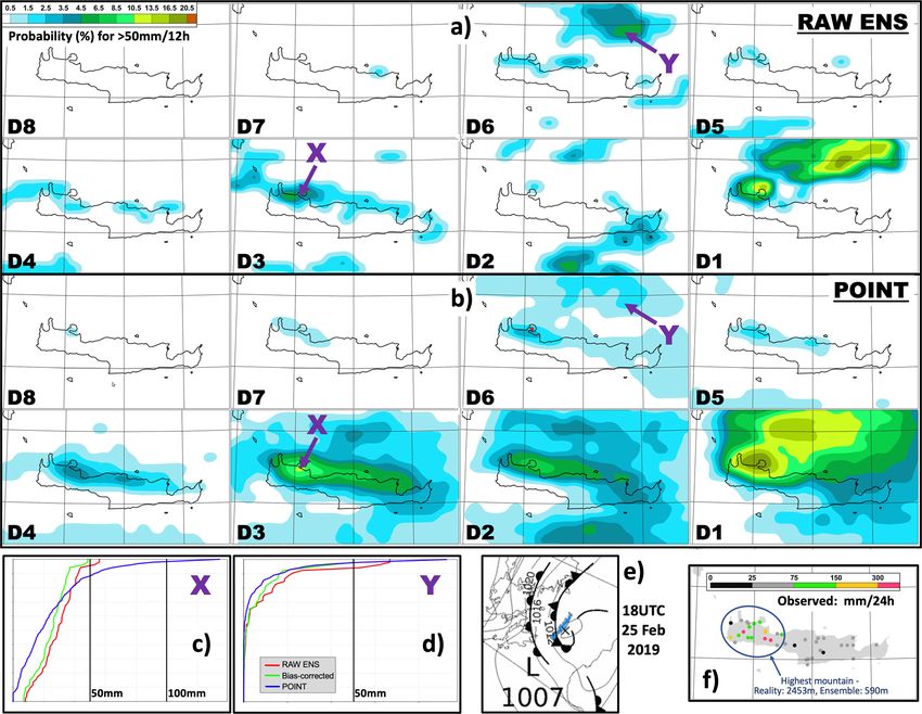
ARTICLE                                                                 COMMUNICATIONS EARTH & ENVIRONMENT | https://doi.org/10.1038/s43247-021-00185-9

W
             eather forecasts nowadays rely heavily on computer-                                       showers/convection) arises from localised pockets of rapid ascent,
             based models, i.e. numerical weather prediction                                           which are typically hundreds of metres to kilometres across. So
             (NWP)1, and commonly an ensemble of predictions is                                        during convection rainfall rate sub-grid variability, on GM scales,
used, to represent uncertainties2. Due to computational power                                          can be very large indeed13 (Fig. 1b, c).
limitations, a gridbox in the best operational global ensembles                                           Rainfall totals arise from integrating rainfall rates over time.
currently spans about 20 km by 20 km in the horizontal (here-                                          Sub-grid variability in totals mostly reduces in proportion to
after: “GM scales” = Global Model scales). So NWP forecasts do                                         period length. Let us consider, as in many rainfall PP studies,
not output rainfall (for example) at specific sites, that most cus-                                     daily to sub-daily time periods (e.g. 6, 12, 24 h), and focus on
tomers require, but instead “average rainfall” for much larger                                         convection. The intensity, dimensions, density, genesis rate,
gridboxes. This disconnect is an important forecasting problem,                                        longevity, and speed of movement of convective cells all impact
which this study addresses. To elaborate, we introduce here the                                        upon the sub-grid variability in totals. For example, cells moving
notion of “sub-grid variability”, to mean the variation seen                                           with speed V, that retain intensity and dimensions for a period t,
amongst all point values observed within the same model gridbox.                                       will deliver stripes in a totals field of length V*t. Typical values of
If sub-grid variability is low then raw NWP forecasts can provide                                      V and t might be 15 m s−1 and 1 h, giving a stripe 54 km long,
accurate forecasts for points. But if sub-grid variability is high                                     which is much greater than GM scales. In such situations we thus
such forecasts inevitably fail.                                                                        get sub-grid variability primarily in one dimension (Fig. 1b). In
   The most common strategies to address sub-grid variability pro-                                     the limiting case of slow-moving cells, where V → 0, we retain
blems are using a much higher resolution model (e.g. ∼2 km*2 km)                                       (large) sub-grid variability in two dimensions (Fig. 1c), and
to minimise them3, or using calibrated post-processing (PP) techni-                                    sometimes many locations within “wet gridboxes” stay dry.
ques to statistically convert from gridbox to point forecasts4–6. For                                     The embodiment of ecPoint is that features of the NWP gridbox
predicting rainfall, the parameter central to this article, high-                                      forecast output (and other global datasets) can tell us what degree of
resolution models, whilst showing much more realistic-looking spa-                                     sub-grid variability to expect. For example, NWP output commonly
tial patterns, and exhibiting improvements in forecast skill7,8, have                                  subdivides rainfall into dynamics-driven and convective, and then for
limited geographical coverage. This is because of computational                                        convective cases shower movement speed can be approximated by
constraints, which imply that one such model might only cover                                          (e.g.) the 700 hPa wind speed. So by using the convective rainfall
~0.2% of the world. For global coverage PP techniques are a better                                     fraction and the 700 hPa wind speed (two “governing variables”) we
prospect, and they have historically performed well in improving                                       can distinguish each of the three “gridbox-weather-types” on Fig. 1,
forecasts of dry weather6,9, but as previous authors themselves                                        to anticipate a priori the expected sub-grid variability, and accord-
acknowledge, many challenges and issues remain (Table 1). Table 1                                      ingly convert each forecast for each gridbox into a probabilistic point
also highlights how our brand-new approach, described in this study,                                   rainfall prediction (going from red to blue on Fig. 1 PDFs). To our
addresses these points. Ours is a non-local gridbox-analogue                                           knowledge this general approach, based on first principles of pre-
approach, formulated via the principles of conditional verification10,                                  cipitation generation, has not been used before except in a limited
with some structural similarities to quantile regression forests11,12.                                 way for nowcasting14 (Table 1, row 11). Another powerful feature of
We call the method “ecPoint”—“ec” for ECMWF, i.e. the European                                         our approach is that each gridbox-weather-type is also associated, via
Centre for Medium-Range Weather Forecasts, and “Point” for point                                       calibration, with a gridscale bias-correction factor.
forecasts.                                                                                                The logic outlined above could be successfully applied to a
   Sub-grid variability in rainfall is itself very variable (Fig. 1) and                               single deterministic forecast but in NWP ensembles furnish the
relates closely to the weather situation. There are clear-cut phy-                                     most useful predictions2,15. So instead we apply separately to each
sical reasons for this. Dynamics-driven (large-scale) rainfall, often                                  ensemble member, creating an ensemble of probabilistic realisa-
related to atmospheric fronts, arises from steady ascent of moist                                      tions (or “ensemble of ensembles”) that we merge to give the final
air across regions typically larger than GM scales (Fig. 1a). As                                       probabilistic point forecast. Whilst Fig. 1 shows just three grid-
rainfall rates mirror ascent rates, rainfall rate sub-grid variability                                 box-weather-types, ECMWF’s current ecPoint-Rainfall system
tends to be small. Conversely instability-driven rainfall (i.e.                                        uses 214 such types, defined in decision tree form.

 Table 1 What (previously reported) challenges/issues do classical post-processing methods often face?

 Challenge/issuea                                                                                     Related characteristics of ecPoint
 1  Calibration requires ≳20 years of observations5,6,46,48–51             Vast training datasets come from just 1 year of data
 2  Calibration requires ≳20 years of ensemble re-forecastsb 6,46,49,50,52 1 year of re-forecasts, from just one (Control) run, for up to 48 h lead
                                                                           times, is sufficient
 3 Lack of climatological stationarity potentially a problem33,46,51,53,54 1 year of training is short enough to avoid this
 4 Forecasts not possible where no training data is available46            Forecasts can be created for all locations
 5 Distribution fitting often used may not mirror real data5,6,12,55        Nonparametric methods are used
 6 Distribution fitting struggles to represent tails well5,6,51,55,56       There are no constraints on tail structure
 7 Difficult to improve forecasts of extremes5,6,9,12,52,55–59              Forecasts of ‘extremes’ are substantially better
 8 Occasional errors in training data may contaminate forecasts61          Impacts of such errors are nil or negligible
 9 No pointers regarding “reasons” for model errors/biases                 “Mapping functions” used denote model characteristics
 10 Post-processed spatial output may require smoothing9,46                Aesthetically smooth fields arise naturally
 11 Large scale/convective precipitation are not disaggregated             An intrinsic and valuable facet of the method
 12 Can different modelling systems’ biases be compared and                Decision tree reproduction can facilitate this
    addressed?62,63
 13 Coverage is not globalc                                                Coverage is global
 aWhich issues are relevant depends on the method. Citations denote where an issue has been highlighted, without a clear mechanism for addressing. Studies in which an issue has been highlighted with a
 mechanism for addressing are as follows: issue no. 612, issue 760,61, issue 960, issue 1114, issue 1328.
 bIn the U.S. calibration is the main driving force for running re-forecasts (Tom Hamill, personal communication). ECMWF’s re-forecast strategy is different.
 cBesides the one study28 no other cited work can have global coverage.

2                COMMUNICATIONS EARTH & ENVIRONMENT | (2021)2:132 | https://doi.org/10.1038/s43247-021-00185-9 | www.nature.com/commsenv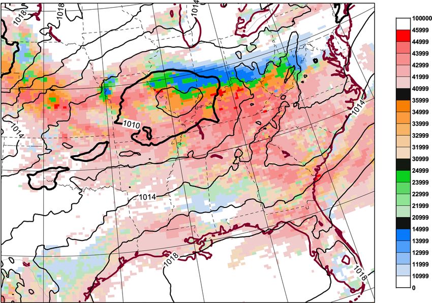
COMMUNICATIONS EARTH & ENVIRONMENT | https://doi.org/10.1038/s43247-021-00185-9 ARTICLE
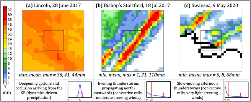
Fig. 1 Three cases of 24 h radar-derived rainfall totals (mm) in the UK illustrating different types of sub-grid variability. a–c Each denote a different
case: cells measure 2 × 2 km, black denotes coasts, full frames are 54 × 54 km; legend for 24 h rainfall (mm) applies to all. Central black boxes denote an
ECMWF ensemble gridbox (18 × 18 km), for which minimum, mean, and maximum rainfall is shown beneath. Named locations lie approximately mid-panel;
all are in regions where relatively flat topography makes radar-derived totals more reliable. Bottom row explains the synoptic situations; inset graphs show,
conceptually, how a raw ensemble member forecast (red) for the box should be converted by ecPoint into a probability density function (PDF) for point
values (blue) within the box; pink line denotes the 95th percentile; x-scale is linear. Flash floods affected the two regions with red pixel clusters in (c)64.
Radar images are from netweather.tv.
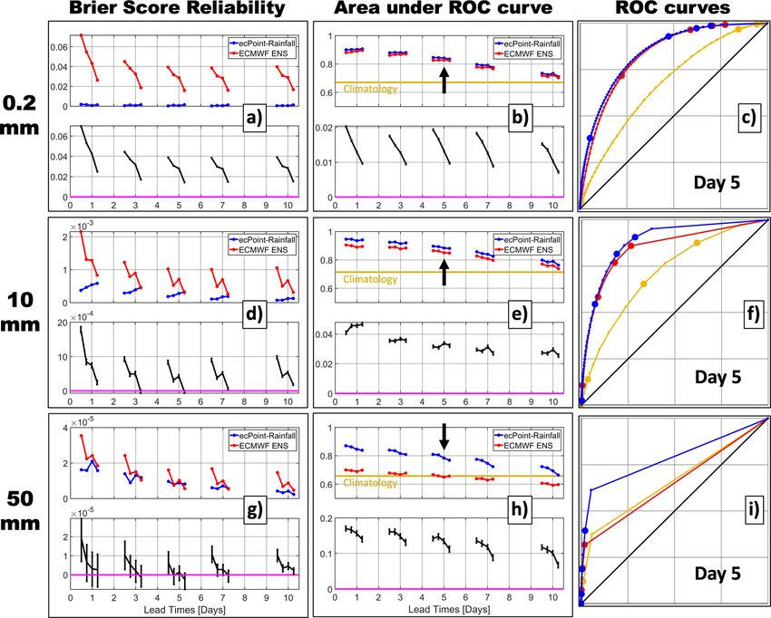
Calibration for the post-processing is achieved not by using radar climatological probabilities (even if these were not available
data, but instead rain gauge observations from across the world, in everywhere). Figure 2 displays results for three 12 h accumulation
conjunction with short-range Control run re-forecasts, in an inno- thresholds: 0.2 mm (“dry or not”), 10 mm (“wet”), and 50 mm
vative, inexpensive, non-local procedure (Table 1, rows 1, 2). (“extreme, with flash flood potential”).
Applications of ecPoint include the many spheres that would For both metrics and almost all lead times ecPoint out-
benefit from improved probabilistic point forecasts. For rainfall, performs the raw ensemble. Reliability improvements are
flash flood prediction is one application, given that we achieve particularly striking for the 0.2 mm threshold; this relates to use
much improved forecasts of localised extremes, as will be shown. of a zero multiplier for gridbox totals in convective rainfall
ECMWF has been delivering real-time experimental ecPoint- situations (e.g. Fig. 1c PDFs). The ecPoint lead-time gains22 from
Rainfall products to forecasters since April 2019. ROCA, for 0, 10, and 50 mm thresholds are, respectively, about 1,
2, and 8 days (centring on day 5). The particularly large gains for
high totals relate, primarily, to weather-type-dependant inclusion
Results of large multipliers for the raw NWP forecast gridbox rainfall (e.g.
Verification. To have value PP techniques must improve upon raw see blue curve tails on Fig. 1b, c PDFs). To put these results into
NWP forecasts. So the performance of 1 year of retrospective context, NWP improvements have historically delivered a lead-
forecasts from both the raw NWP and ecPoint-Rainfall systems was time gain of about 1 day per decade1,23. To have more than “weak
compared, using as truth 12 h rainfall observations from both potential predictive strength”, ROCA must be some way above
standard SYNOP reports (global coverage) and specialised high- the zero-skill baseline24. So, for 0.2 and 10 mm/12 h thresholds
density datasets (certain countries, mainly European16). Verification raw ensemble and ecPoint have potential predictive strength out
and calibration periods were separate. Although raw model output to ~days 7–10. For 50 mm this limit is at least day 5 for ecPoint,
does not pertain to point values, it is very common to verify using whereas the raw ensemble has limited utility even on day 1. ROC
them, as in ECMWF’s two headline measures for precipitation17,18. curves show that for 10 and 50 mm thresholds the ecPoint
Here we utilise categorical verification because threshold system’s added value, expressed as ROC area impact, stems from
setting is common for applications and because forecast products a better handling of the wet tails of the inferred sub-grid point
reflect this (see the sections “Case study examples” and rainfall distributions—e.g. 98th/99th percentiles (see also Supple-
“Methods”). In this framework, the two fundamental aspects to mentary Discussion Section 1 and a more detailed ROC curve
assess are reliability (i.e. when x% probability is forecast is the presentation in Supplementary Fig. 1).
event observed on x% of occasions?) and the capacity to Equivalent ROCA plots for the tropics only, where site
discriminate events. For these, we use respectively, the Reliability climatologies should be more similar, indicate for point rainfall
component of the Brier Score19, which is an integral measure of larger absolute increases in ROCA and larger lead time gains
reliability across all issued probabilities, and area under the (ROCA climatological skill here is almost unchanged). Nonetheless
relative operating characteristic (ROC) curve (ROCA)15,20. similar plots for just extratropical regions exhibit lead time gains
When verifying probabilistic grid-based forecasts against point only ~25% less than the quoted global values. Overall, the slightly
measurements one cannot achieve perfect discrimination, because better tropical performance arises because for convective weather
of sub-grid variability. We believe that relative to other types, which are more common here, there is more value to be
discrimination metrics ROCA, also used operationally18, is much added, which ecPoint does. In improving “convective precipita-
more immune to limitations placed by this. ROCA can exhibit tion” we have addressed the world’s number one NWP issue25.
false skill when site climatologies differ21, so whilst the objective Reliability, particularly for the raw ensemble, is better for leads
here was to ascertain ecPoint’s added value, by comparing ROCA >day 1, which may relate to ensemble perturbations being
scores, a “zero-skill” baseline was also needed, based on local optimised for the medium range. A model spin-up issue also
COMMUNICATIONS EARTH & ENVIRONMENT | (2021)2:132 | https://doi.org/10.1038/s43247-021-00185-9 | www.nature.com/commsenv 3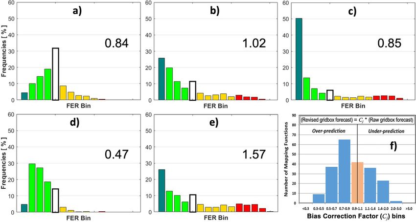
ARTICLE                                                  COMMUNICATIONS EARTH & ENVIRONMENT | https://doi.org/10.1038/s43247-021-00185-9

Fig. 2 Category-based verification for 1 year of global gauge observations of 12 h rainfall. a–c, d–f, g–i Signify thresholds of ≥0.2, ≥10, ≥50 mm/12 h,
respectively. Red/blue denote raw/point rainfall forecasts, respectively; black profiles beneath denote differences signed such that positive implies point
rainfall is better (magenta = 0), with 95% confidence intervals taken from bootstrapping with simple random replacement65 of daily datasets (1000x). a,
d, g show Brier Score reliability component, 0 is optimal; points intersecting vertical gridlines denote 12 h periods ending 00 UTC, others are for end times
(left to right) of 12, 18, 06 UTC. b, e, h show area under the ROC curve as a measure of system discrimination ability, larger is better, upper limit is 1; point
meaning as for left column; yellow denotes a “baseline”, for climatology-based forecasts (for sites where that is available); arrows denote lead time used
for right column. c, f, i show day 5 ROC curves (false alarm rate = 0–1 (x) versus hit rate = 0–1 (y)), including climatology; large spots signify probabilities
of 2% (topmost), 4%, 10% and 51%. Percentiles 1, 2, …, 99 are used for point rainfall and for climatology.

affects the leftmost points (T + 0–12 h). For the 50 mm threshold,                but not reliability for larger totals (reference our Fig. 2d, e).
although ecPoint looks better overall, the absence of significant                  Verification of very large totals was missing. The study in effect
reliability gains at most lead times probably relates to information              assumes just one weather type. We attribute our much better
loss in the forecast distribution tail, arising because the largest               performance to using multiple types.
percentile verified is 99th, even though 99.98th is computed.                         Meanwhile, in two 1-year verification comparisons with
Although areal warnings of flash flood risk are now issued for                      convection-resolving limited area ensembles, with and without
relatively low point probabilities, we nonetheless expected little                modern post-processing applied, for two relatively mountainous
user interest in chances of 75 mm/24 h
   The oscillations seen on all panels on Fig. 2 are a function of                was widely reported, with up to 373 mm/24 h locally (Fig. 3f).
UTC time, and relate to irregular observation density coupled                     Extensive damage occurred, including the collapse of 2 bridges29.
with outstanding systematic errors in forecasts of the diurnal                    In the preceding days raw ensemble rainfall forecasts (Fig. 3a)
cycle of convection26,27. Ongoing work with a 6 h accumulation                    were noisy, jumpy (“Jumpy” is a term regularly used by fore-
period and a governing variable of local solar time is helping                    casters: it refers to when forecasts for a given time, produced by
ecPoint to address this deficiency.                                                consecutive model runs, are inconsistent with one another.) and
   In surveying post-processing activities worldwide (see also                    confusing, with relatively low probabilities of large totals. In
Supplementary Discussion Section 2) we uncovered just one                         relative terms ecPoint (which of course uses the raw ensemble)
global method for which a verification comparison with ecPoint                     performs much better (Fig. 3b). First, fields are smoother. Second,
was meaningful. That study28 improved reliability but not                         probabilities grow over time, are more consistent and are less
resolution for small totals (reference our Fig. 2a, b) and resolution             jumpy. Third, ecPoint’s largest probabilities were more focussed

4             COMMUNICATIONS EARTH & ENVIRONMENT | (2021)2:132 | https://doi.org/10.1038/s43247-021-00185-9 | www.nature.com/commsenv
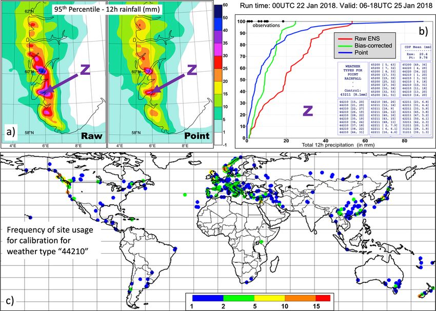
COMMUNICATIONS EARTH & ENVIRONMENT | https://doi.org/10.1038/s43247-021-00185-9                                                               ARTICLE

Fig. 3 Evolution of raw ensemble and ecPoint forecasts for a flooding event in Crete. a Forecast probabilities (%), for 12–24 UTC 25 February 2019, for
rainfall >50 mm, from raw ensemble; D8, D7, …D1 (for days 8, 7, …, 1) denote data times of 00UTC on, respectively, 18, 19 … 25 February. b As a but for ecPoint.
c CDFs for 12 h rainfall from the respective D3 forecasts for site X shown on (a) and (b), for raw ensemble gridbox totals (red), bias-corrected gridbox totals
(green) and point rainfall (blue), for 12–24UTC 25th (y-axis spans 0–100% and lies at x = 0 mm). d As c but for D6 for site Y. e UK Met Office surface analysis
for 18UTC 25th (Crete in blue). f Gauge observations of 24 h rainfall: 00–24UTC 25 February 2019 (very few 12 h totals are available here).

on western Crete where floods occurred. And fourth, probabilities                 Typically, ecPoint’s wetter tail will cross the raw ensemble tail
are higher overall. Conversely, we expect an orographic                          around 85% (e.g. Fig. 3c). But here, even for the 95th percentile,
enhancement shortfall in the raw model (due to lower mountain                    in the north–south chain of maxima (Fig. 4a), ecPoint values are
peaks, Fig. 3f) which was apparently not rectified by ecPoint.                    still lower. The reason here is not outliers; it is instead the
Nonetheless, Fig. 3a, b suggest that forecasters could have pro-                 adjustment for an expected large over-forecasting bias: compare
vided much better warnings here using ecPoint fields, and ver-                    green and red lines in Fig. 4b. Specifically, the main gridbox-
ification results in Fig. 2 for 50 mm/12 h suggest that this                      weather-type diagnosed here (labelled “44210”, see also Supple-
conclusion has general validity.                                                 mentary Fig. 2) is itself associated with a substantial gridscale
   The probabilities for a large threshold are usually higher in                 bias-correction. Norwegian forecasters, based on experience, also
ecPoint output because PP tends to extend the wet tail, at least in              envisaged that rain in this situation would be over-forecast
(partially) convective situations, as on the cumulative distribution             (personal communication, Vibeke Thyness). Nearby gauge
function (CDF) in Fig. 3c. This extension requires, for                          observations (black dots, Fig. 4b), and radar-derived totals seem
mathematical reasons, some intra-ensemble consistency. In an                     to support better the ecPoint forecasts.
alternative case of wet outlier(s), probabilities within the tail can               Figure 4c shows that during calibration the training data for
be reduced—e.g. Fig. 3d. This is because gauge totals following                  type “44210” came mostly from mountainous regions near coasts,
convection are most likely to be less than the forecast gridbox                  consistent with topographic convective triggering being the
value, due to the non-Gaussian structure of the expected point                   rainfall generation mechanism. A likely reason for the over-
total distribution (e.g. see PDFs on Fig. 1b, c).                                prediction is that in reality when low-CAPE airmasses impinge
   Figure 1c illustrates smaller-scale flash flood events that were                on mountains convective cells take time to grow and rain out,
also consistently forecast and localised much better by ecPoint                  whilst in global NWP rainfall is immediate. ecPoint highlights
than by the raw ensemble, from 5 days out.                                       quantitatively the impact. In turn the large biases identified raise
   Another feature of ecPoint PP is illustrated in Fig. 4a, b which              important questions about how, for example, related latent heat
is for a cyclonic, convective, winter-time case in Norway.                       release overestimates might reduce subsequent broadscale

COMMUNICATIONS EARTH & ENVIRONMENT | (2021)2:132 | https://doi.org/10.1038/s43247-021-00185-9 | www.nature.com/commsenv                                       5
ARTICLE                                                 COMMUNICATIONS EARTH & ENVIRONMENT | https://doi.org/10.1038/s43247-021-00185-9

Fig. 4 Day 4 rainfall forecasts for a southwest Norway case, with a calibration site usage map. a 95th percentile of 12 h rainfall (mm) from data time
00UTC 22 January 2018 for 06–18 UTC on 25th, from raw ensemble (left) and ecPoint (right). b CDFs of 12 h rainfall for site Z shown on a, for same data/
valid times as a, for raw ensemble gridbox totals (red), bias-corrected gridbox totals (green) and point rainfall (blue); table inset shows: assigned weather
type as a 5-digit code, then [member number, forecast rainfall in mm]. c Locations of calibration events used to define the gridbox-weather-type “44210”.

predictability. The Crete case (Fig. 3) differs because rainfall there          physical meaning; the many other attractive features of ecPoint
had a smaller convective component.                                             stem from this (Table 1). “Weather type” importance has long
   These examples show how ecPoint is rich in physically realistic              been recognised, but in the form of country-scale circulation
complexity, which helps deliver much better forecasts on average.               patterns33,34 which imposes huge constraints on training data size
Similarly using gridbox-weather-types increases understanding of                compared to our gridbox-weather-type approach.
model behaviour. Other PP methods do not generally have these                      Whilst ecPoint can predict local extremes via “remote learn-
desirable characteristics.                                                      ing”, the lack of global record conditions in training data could
   Figures 3a, b and 4a (and Supplementary Figs. 3a–t and 4a–t)                 very occasionally be a constraint. However, using mapping
provide examples of the operational ECMWF products. Users can                   functions means that new global records can be predicted whilst
select their own thresholds, compare raw and point forecast fields,              in some other PP methods they cannot12.
and reference user guidelines30.                                                   For specific sites alternative MOS-type techniques (model output
                                                                                statistics) might provide better forecasts than ecPoint, if local
Discussion                                                                      topography and/or meteorological characteristics are especially
We describe a completely new PP approach to forecasting                         unusual. Similarly, local verification will inevitably reveal some
weather at sites—ecPoint—to meet customer need in ways that                     regional differences in ecPoint performance. These should however
pure global NWP cannot. Our focus has been on rainfall                          stimulate future upgrades to the governing variables and the deci-
(renowned to be particularly challenging31,32) but the philosophy               sion tree. More complexity can certainly be included, but in time
applies also to other variables. Verification results are very posi-             greater observation coverage will be needed to support this. We
tive, even for 50 mm/12 h. Comparable techniques are very                       therefore plan to exploit more high-density observations, including
scarce. We beat the only real competitor, and match or beat two                 new crowdsourced data35, potentially including periods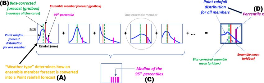
COMMUNICATIONS EARTH & ENVIRONMENT | https://doi.org/10.1038/s43247-021-00185-9                                                                    ARTICLE

Fig. 5 Mapping function examples, and the bias correction factor distribution. a–e Mapping function examples from the current operational forecast
system shown as histograms; large digits show implicit bias correction factors C. Dark green, green, white, yellow, and red bars denote, respectively, FER
ranges for “mostly dry” ( 0.75, moderate
CAPE (convective available potential energy), strong steering winds, (c) for Pconv > 0.75, moderate CAPE, light winds, (d) for Pconv > 0.75, large forecast
totals, moderate winds, low CAPE (=weather type identifier “44210”—see Fig. 4b, c), (e) for 0.25 < Pconv < 0.5, modest forecast totals, moderate winds,
moderate CAPE. f C value distribution for all 214 mapping functions.

meaningful physical insights. It is vital for NWP development to               remain as strong as ever. The difference now is that by simulta-
understand the differences between raw and bias-corrected                      neously exploiting the strong synergistic relationship with ecPoint
gridbox values. Figure 4b, c provided a clear example of why.                  we can secure much larger forecast improvements for everyone.
Such insights are a major advantage of the ecPoint approach.
   ecPoint has many other diverse applications. Its output is                  Methods
currently being blended with post-processed high-resolution                    Calibration. In general PP methods need to be calibrated. This requires observa-
limited-area ensemble forecasts37, to exploit their better repre-              tions. For ecPoint we use (unadjusted) rain gauge data as this represents points, is
                                                                               commonly used for operational verification16–18, and has extensive worldwide
sentation of some topographic effects (reference Fig. 3f), to                  coverage (over land where rainfall forecast needs are by far the greatest). Whilst
deliver better forecasts overall and to seamlessly transition into             issues do exist with gauge data44 other data types would present far more limita-
the medium range. Meanwhile historical probabilistic point                     tions and complications.
rainfall and point temperature re-analyses will be created from                    To calibrate we appeal to the concept of conditional verification to create a
                                                                               separate ‘mapping function’ (M) for each of the m possible combinations of
the gridscale global re-analysis called ERA538, delivering unpar-              governing variable ranges (i.e. the m gridbox-weather-types). Each such function
alleled representativeness back to 1950. The pointwise climatol-               aims to represent possible outcomes, and indeed a distribution, of point rainfall
ogies so-derived will themselves have numerous applications,                   within a gridbox and so each should represent a different type of sub-grid
such as providing a reference point (independent of model ver-                 variability. In our very simple Fig. 1 example there would be three categories (A–C)
sion/resolution) to see if ecPoint forecasts are locally extreme, via          of “gridbox-weather-type” (or “type”) which would have governing variable
                                                                               characteristics like these (Pconv = fraction of total precipitation forecast to be
the “extreme forecast index” philosophy39. Thereby ecPoint                     convective, V700 = 700 hPa wind speed):
forecasts become even more relevant for flash flood prediction.
                                                                                  ●    A: Pconv < 0.5
Other applications include inexpensive downscaling of climate                     ●    B: Pconv > 0.5 and V700 > 5 m s−1
projections40, global tests of hypotheses such as “do cities affect               ●    C: Pconv > 0.5 and V700 < 5 m s−1
rainfall”41, and quality-control of observations42 using a point-
                                                                                  Then mapping functions MA, MB, MC would represent PDFs of point rainfall
CDF-based acceptance window. Improved bias-corrected feeds                     within a gridbox for, respectively, types j = A–C. To create, in the general case, m
into hydro-power and hydrological43 models are also objectives.                mapping functions we need to allocate, to one of the m types, each and every
   So why is ecPoint “low cost”? Providing the control run fore-               observation (r 0 ) taken during a pre-defined period—1 year is sufficient—and over a
casts we use for calibration is orders of magnitude cheaper than               pre-defined region, ideally the world. At the same time, we must relate these to
                                                                               forecast gridbox rainfall totals (G) that inevitably differ, and to do this we introduce
providing the multi-year ensemble re-forecasts needed by many                  a nondimensional metric, the “forecast error ratio” (FER):
other PP methods. And in operations, ecPoint’s own computa-
tions are many orders of magnitude cheaper than global NWP                                         FER ¼ ðr 0  GÞ=G       ðrequires G ≥ 1 mmÞ                ð1Þ
alternatives (which in 2021 are very far from being operationally                                              R1
                                                                               So that M ¼ Mðx ¼ FERÞ with 1 Mdx ¼ 1:
viable anyway). Nonetheless, PP methods would be worthless                        Naturally we assign each r 0 value to a gridbox based on location and assign a
without high-quality NWP forecasts to provide the input. Indeed,               companion type to that gridbox at that time using values of the selected governing
the investment and development needs of global ensembles                       variables. Short-range (unperturbed) control run forecasts provide these values,

COMMUNICATIONS EARTH & ENVIRONMENT | (2021)2:132 | https://doi.org/10.1038/s43247-021-00185-9 | www.nature.com/commsenv                                              7
ARTICLE COMMUNICATIONS EARTH & ENVIRONMENT | https://doi.org/10.1038/s43247-021-00185-9
Fig. 6 Schematic showing how an ecPoint (rainfall) forecast is constructed for one gridbox at one time, and outputs that can be created. Blue boxes
each show probability density functions (PDFs); bracketed set of 5 represents some ensemble member forecasts, box after “=” shows the final merged
“ensemble of ensembles” product. Input gridbox (average) values are shown by red lines and bias-corrected equivalents by dashed green lines; blue curves
show ecPoint point PDFs. Pink/purple lines denote percentiles extracted from the respective blue PDFs. Lowermost box shows together the 95th
percentiles for each member’s point PDF. The primary (single value) ecPoint outputs one can create are labelled in black: (A) the weather type identifier
index for an ensemble member, (B) bias-corrected gridbox rainfall forecast for a member, (C) the median rainfall of the 95th (or other) percentiles from all
members’ point PDFs, (D) the full ensemble’s point PDF rainfall value at a given percentile x. Output charts for forecasters currently derive from (D) with x
= 1, 2, …, 99%. The same general principles depicted here also apply for other variables (besides rainfall).
and G = Gcontrol. Then, after discarding cases with Gcontrol < 1 mm for stability/ factor45. Removing location facilitates the generation of immense training datasets
discretization reasons, each remaining (Gcontrol, r 0 ) pair furnishes one FER value (matching recommendations46) that deliver on average ~104 cases for each
for the said gridbox-weather-type. By accumulating these we ultimately generate mapping function. An example will illustrate the powerful implications of this for
one FER PDF for each mapping function, i.e. M1, … Mj, … Mm. These form the ecPoint. Consider a Swedish site experiencing a gridbox-weather-type that is a one-
calibration procedure output; five examples are shown in Fig. 5a–e. Equation (1) in-5-year event there (e.g. including locally extreme convective available potential
indicated that NWP “over-prediction” for a rain gauge site was represented by FER energy, i.e. CAPE). Such types do occur much more often globally, enough to
< 0 (see dark green and green bars), and “under-prediction” by FER > 0 (see yellow deliver ~104 calibration cases for that type in 1 year of global data. Handling this is
and red bars). computationally straightforward, and moreover the huge case count facilitates our
In Fig. 5 examples, sub-grid variability magnitude depends strongly on the hyper-flexible non-parametric approach. To match this in a simple deterministic
gridbox-weather-type. Figure 5a–c, for example, broadly correspond, respectively, MOS approach4, or a state-of-the-art ensemble approach with 50 supplementary
to examples in Fig. 1a–c. Variability is lowest in Fig. 5a (distribution roughly sites47, would conversely require the impossible—i.e. data for the last 50,000 or
Gaussian) and highest, with the greatest likelihood of zeros, in Fig. 5c (distribution 1000 years, respectively.
roughly exponential). This correspondence supports the use of worldwide gauge
observations for our “non-local” calibration. In standard convective situations Forecast production. ecPoint forecast production relies on converting Eq. (1) for
(Fig. 5b, c) “good forecasts” (white bar) are evidently rare, whilst substantial under- FER into a vector form: r 0 becomes Fi(r), a probabilistic point forecast of rainfall r
prediction (red), which could lead to “unexpected” flash floods, is relatively
from member i for the period/gridbox in question, Gi is that member’s raw rainfall
common, especially when steering winds are light (Fig. 5c).
forecast, and FER becomes Mi (FER), the mapping function selected for that
Physical reasoning and case studies suggest that gridscale bias in raw NWP
member. With rearrangement:
forecasts can also depend strongly on gridbox-weather-type. As well as predicting
sub-grid variability ecPoint also corrects for this bias. The grid-scale bias correction Fi ðrÞ ¼ ð1 þ Mi ðFERÞÞGi where Mi 2 fM1 ; ¼ ; Mm g ð3Þ
factor (Cj) is implicit in each mapping function; it derives from the “expected
value” of the associated FER:
The final probabilistic rainfall forecast vector F, for a point in a given gridbox, is
Z 1 then simply derived using all n ensemble members:
Cj ¼ 1 þ x Mj dx
1 ð2Þ 1 n
F¼ ∑ Fi ðrÞ ð4Þ
ðmean rainfall observedÞ=ðmean rainfall forecastÞ for type j: n i¼1
The ensemble of ensembles computed operationally currently utilises m = 214
Figure 5f shows the range of Cj values for all mapping functions currently used; mapping functions, with the FER PDF for each simplified into 100 possible
for some weather types the ECMWF model seems to markedly over-predict or outcomes, for computational speed. So for each gridbox/period we arrive at 5100
under-predict rainfall (e.g. Fig. 5d and e, respectively). This is key for ecPoint and is possible realisations (100*51 members), which are then distilled into percentiles
informative also for forecasters and model developers. Although not a definitive 1,2,…,99 for forecasting. Figure 6 represents the above schematically, whilst Fig. 7
inference, Fig. 5f supports the working assumption27 that on average the ECMWF is an example of the geographical distribution of weather types for one ensemble
model over-predicts rainfall (although gauge undercatch44 may be a mitigating member.
factor). The equivalence on line 2 of Eq. (2) assumes ∂Cj/∂G ≅ 0. The larger the Supplementary Methods Section 7 includes a more detailed discussion of the
range of G values the less likely this is to be valid. We reduce ranges by using G as a computational details, and of how the challenges of operational production can be
governing variable for each type j, thereby increasing the efficacy of our model bias addressed. Then in Supplementary Methods Section 8 we discuss graphical output
interpretation. options and forecaster use of those. Also included there, with verifying data, are
A feature of our method is the freedom for the user to select, test, and examples of how raw ensemble and ecPoint forecast distributions differ, at various
incorporate any variable that can influence rainfall sub-grid variability and/or bias. lead times in different synoptic settings, over large extratropical and tropical
The following variable “classes” are included: “raw model”, “computed”, domains (Supplementary Figs. 3 and 4). Supplementary Fig. 5 then demonstrates
“geographical”, “astronomical”. The first two relate directly to NWP output, the how significant these distribution differences can be at different leads.
second two to other datasets. In Supplementary Methods Sections 1–3 these classes
are discussed in detail, with examples (see also Supplementary Table 1), and we
discuss the assumptions implicit in the approach. Then in Supplementary Methods Data availability
Sections 4–6 we describe the semi-objective strategy to define governing variable Data specific to case Figs. 1c, 3, 4, 7 and verification scores supplementary to Fig. 2 can be
breakpoints and thus decide upon the full set of gridbox-weather-types and the found at: 10.5281/zenodo.4728765. ECMWF does not have the legal rights to re-
related decision tree (a portion is shown in Supplementary Fig. 2). There is also distribute worldwide rainfall observations as used for Fig. 2; some observational data can
reference to a new open source graphical user interface (GUI) for performing be obtained from the WMO GTS (World Meteorological Organisation Global
ecPoint calibration and for building the decision tree. Telecommunication System) and from some national archives. Raw model output used
Unlike classical methods, location is not used in the calibration. This concurs in this study is stored in the ECMWF archive (https://www.ecmwf.int/en/forecasts/
with tests of site separation importance that allocate only 2% weight to this
8 COMMUNICATIONS EARTH & ENVIRONMENT | (2021)2:132 | https://doi.org/10.1038/s43247-021-00185-9 | www.nature.com/commsenvCOMMUNICATIONS EARTH & ENVIRONMENT | https://doi.org/10.1038/s43247-021-00185-9 ARTICLE Fig. 7 Example of weather types assigned operationally for a Control run precipitation forecast over the USA for a given 12 h period. Data time is 00UTC 30 July 2020, valid time is 12–24UTC on 30th. Each colour denotes a range of gridbox-weather-type identifiers—see legend and Supplementary Fig. 2 (representing all 214 individually is impractical). Blue, green, orange, red show, respectively, Pconv (level 1 on Supplementary Fig. 2)
ARTICLE                                                         COMMUNICATIONS EARTH & ENVIRONMENT | https://doi.org/10.1038/s43247-021-00185-9

26. Bechtold, P. et al. Representing equilibrium and nonequilibrium convection in          56. Friedrichs, P., Wahl, S. & Buschow, S. Postprocessing for extreme events. In
    large-scale models. J. Atmos. Sci. 71, 734–753 (2014).                                     Statistical Postprocessing of Ensemble Forecasts (eds Vannitsem, S., Daniel S.
27. Haiden, T. et al. Use of In Situ Surface Observations at ECMWF. Technical                  Wilks, D. S. & Messner, J. W.) 347 (Elsevier, 2018).
    Memorandum 834 (ECMWF, 2018).                                                          57. van Straaten, C., Whan, K. & Schmeits, M. Statistical postprocessing and
28. Ben Bouallegue, Z., Haiden, T., Weber, N. J., Hamill, T. M. & Richardson, D.               multivariate structuring of high-resolution ensemble precipitation forecasts. J.
    S. Accounting for representativeness in the verification of ensemble                        Hydrometeorol. 19, 1815–1833 (2018).
    precipitation forecasts. Mon. Weather Rev. 148, 2049–2062 (2020).                      58. Mylne, K. R., Woolcock, C., Denholm-Price, J. C. W. & Darvell, R. J.
29. Kampouris, N. One Dead As Floods Cause Extensive Damage Across Crete (2019)                Operational calibrated probability forecasts from the ECMWF ensemble
    (Greek Reporter, accessed 28 November 2019); https://greece.greekreporter.com/             prediction system: implementation and verification. In Joint Session of 16th
    2019/02/26/one-dead-as-floods-cause-extensive-damage-across-crete-video/.                   Conference on Probability and Statistics in the Atmospheric Sciences and of
30. Owens, R. G. & Hewson, T. D. ECMWF Forecast User Guide (2018). https://                    Symposium on Observations, Data Assimilation and Probabilistic Prediction
    doi.org/10.21957/m1cs7h                                                                    113–118 (American Meteorological Society, 2002).
31. Hemri, S., Scheuerer, M., Pappenberger, F., Bogner, K. & Haiden, T. Trends in          59. Goodwin, P. & Wright, G. The limits of forecasting methods in anticipating
    the predictive performance of raw ensemble weather forecasts. Geophys. Res.                rare events. Technol. Forecast. Soc. Change 77, 355–368 (2010).
    Lett. 41, 9197–9205 (2014).                                                            60. Herman, G. R. & Schumacher, R. S. “Dendrology” in numerical weather
32. Guidelines on Ensemble Prediction Systems and Forecasting. WMO Report                      prediction: what random forests and logistic regression tell us about forecasting
    1091 (2012).                                                                               extreme precipitation. Mon. Weather Rev. 146, 1785–1812 (2018).
33. Van Uytven, E., De Niel, J. & Willems, P. Uncovering the shortcomings of a             61. Herman, G. R. & Schumacher, R. S. Money doesn’t grow on trees, but
    weather typing method. Hydrol. Earth Syst. Sci. 24, 2671–2686 (2020).                      forecasts do: forecasting extreme precipitation with random forests. Mon.
34. Vuillaume, J. F. & Herath, S. Improving global rainfall forecasting with a                 Weather Rev. 146, 1571–1600 (2018).
    weather type approach in Japan. Hydrol. Sci. J. https://doi.org/10.1080/               62. Zadra, A. et al. Systematic errors in weather and climate models: nature,
    02626667.2016.1183165 (2017).                                                              origins, and ways forward. Bull. Am. Meteorol. Soc. 99, ES67–ES70 (2018).
35. Muller, C. L. et al. Crowdsourcing for climate and atmospheric sciences:               63. Swinbank, R. et al. The TIGGE project and its achievements. Bull. Am.
    current status and future potential. Int. J. Climatol. 35, 3185–3203 (2015).               Meteorol. Soc. 97, 49–67 (2016).
36. Haupt, S. E., Pasini, A. & Marzban, C. Artificial Intelligence Methods in the           64. Flash floods hit parts of Gorseinon and Carmarthen. BBC News (2020).
    Environmental Sciences (Springer, 2009).                                                   https://www.bbc.co.uk/news/uk-wales-52602177 (accessed 6 August 2020).
37. MISTRAL Consortium. Definition of MISTRAL Use cases and Services—‘Italy                 65. Wilks, D. S. Statistical Methods in the Atmospheric Sciences (Elsevier, 2019).
    Flash Flood’. 14–16 (2019). http://www.mistralportal.it/wp-content/uploads/
    2019/06/MISTRAL_D3.1_Use-cases-and-Services.pdf (accessed 27 June 2019)
38. Hersbach, H. et al. The ERA5 global reanalysis. Q. J. R. Meteorol. Soc. 146,           Acknowledgements
    1999–2049 (2020).                                                                      D. Richardson provided helpful feedback on earlier drafts of this manuscript, particularly
39. Zsoter, E. Recent developments in extreme weather forecasting. ECMWF                   regarding verification aspects. E. Zsótér put forward useful suggestions regarding
    Newsl. 107, 8–17 (2006).                                                               methodology and output formats. A. Bonet assisted with the operationalization of
40. Kendon, E. J., Roberts, N. M., Senior, C. A. & Roberts, M. J. Realism of rainfall in   ecPoint. A. Bose created the open source graphical user interface (GUI) for calibration.
    a very high-resolution regional climate model. J. Clim 25, 5791–5806 (2012).           M.A.O. Køltzow provided verifying data for the case in Fig. 4.
41. Han, J.-Y., Baik, J.-J. & Lee, H. Urban impacts on precipitation. Asia-Pacific J.
    Atmos. Sci. 50, 17–30 (2014).                                                          Author contributions
42. Sciuto, G., Bonaccorso, B., Cancelliere, A. & Rossi, G. Quality control of daily       T.D.H. invented ecPoint, investigated and selected case studies, calculated climatological
    rainfall data with neural networks. J. Hydrol. https://doi.org/10.1016/j.              forecast skill, enacted statistical tests for Supplementary Fig. 5 and prepared the
    jhydrol.2008.10.008 (2009).                                                            manuscript. F.M.P. investigated governing variable utility, coded up the PP system,
43. Verkade, J. S., Brown, J. D., Reggiani, P. & Weerts, A. H. Post-processing             performed ecPoint calibration and verification, and contributed to drafting of the
    ECMWF precipitation and temperature ensemble reforecasts for operational               manuscript.
    hydrologic forecasting at various spatial scales. J. Hydrol. https://doi.org/
    10.1016/j.jhydrol.2013.07.039 (2013).
44. Sevruk, B. Methods of Correction For Systematic Error In Point Precipitation           Competing interests
    Measurement for Operational Use. WMO Operational Hydrology Report 21                   The authors declare no competing interests.
    (WMO, 1982).
45. Hamill, T. M., Scheuerer, M. & Bates, G. T. Analog probabilistic precipitation
    forecasts using GEFS reforecasts and climatology-calibrated precipitation
                                                                                           Additional information
                                                                                           Supplementary information The online version contains supplementary material
    analyses. Mon. Weather Rev. 143, 3300–3309 (2015).
                                                                                           available at https://doi.org/10.1038/s43247-021-00185-9.
46. Hamill, T. M. Practical aspects of statistical postprocessing. In Statistical
    Postprocessing of Ensemble Forecasts (eds Vannitsem, S., Wilks, D. S. &
                                                                                           Correspondence and requests for materials should be addressed to T.D.H.
    Messner, J. W.) 347 (Elsevier, 2018).
47. Hamill, T. M. & Scheuerer, M. Probabilistic precipitation forecast                     Peer review information Communications Earth & Environment thanks the anonymous
    postprocessing using quantile mapping and rank-weighted best-member                    reviewers for their contribution to the peer review of this work. Primary handling editor:
    dressing. Mon. Weather Rev 146, 4079–4098 (2018).                                      Heike Langenberg
48. Marzban, C., Sandgathe, S. & Kalnay, E. MOS, Perfect Prog, and reanalysis.
    Mon. Weather Rev 134, 657–663 (2006).                                                  Reprints and permission information is available at http://www.nature.com/reprints
49. Wilks, D. S. Statistical methods in the atmospheric sciences: an introduction.
    Int. Geophys. Ser. (1995).
                                                                                           Publisher’s note Springer Nature remains neutral with regard to jurisdictional claims in
50. Wilks, D. S. & Hamill, T. M. Comparison of ensemble-MOS methods using
                                                                                           published maps and institutional affiliations.
    GFS reforecasts. Mon. Weather Rev. 135, 2379–2390 (2007).
51. Mendoza, P. A. et al. Statistical postprocessing of high-resolution regional
    climate model output. Mon. Weather Rev. 143, 1533–1553 (2015).
52. Scheuerer, M. & Hamill, T. M. Statistical postprocessing of ensemble                                     Open Access This article is licensed under a Creative Commons Attri-
    precipitation forecasts by fitting censored, shifted gamma distributions. Mon.                            bution 4.0 International License, which permits use, sharing, adaptation,
    Weather Rev. 143, 4578–4596 (2015).                                                    distribution and reproduction in any medium or format, as long as you give appropriate
53. Wang, Y., Sivandran, G. & Bielicki, J. M. The stationarity of two statistical          credit to the original author(s) and the source, provide a link to the Creative Commons
    downscaling methods for precipitation under different choices of cross-                license, and indicate if changes were made. The images or other third party material in
    validation periods. Int. J. Climatol. 38, e330–e348 (2018).                            this article are included in the article’s Creative Commons license, unless indicated
54. Gutiérrez, J. M. et al. Reassessing statistical downscaling techniques for             otherwise in a credit line to the material. If material is not included in the article’s Creative
    their robust application under climate change conditions. J. Clim 26, 171–188          Commons license and your intended use is not permitted by statutory regulation or
    (2013).                                                                                exceeds the permitted use, you will need to obtain permission directly from the copyright
55. Whan, K. & Schmeits, M. Comparing area probability forecasts of                        holder. To view a copy of this license, visit http://creativecommons.org/licenses/by/4.0/.
    (extreme) local precipitation using parametric and machine learning
    statistical postprocessing methods. Mon. Weather Rev. 146, 3651–3673
    (2018).                                                                                © The Author(s) 2021

10              COMMUNICATIONS EARTH & ENVIRONMENT | (2021)2:132 | https://doi.org/10.1038/s43247-021-00185-9 | www.nature.com/commsenv
You can also read