Directionally Controlled Time-of-Flight Ranging for Mobile Sensing Platforms - Robotics
←
→
Page content transcription
If your browser does not render page correctly, please read the page content below
Robotics: Science and Systems 2018
 Pittsburgh, PA, USA, June 26-30, 2018

Directionally Controlled Time-of-Flight Ranging for
             Mobile Sensing Platforms
                             Zaid Tasneem        Dingkang Wang           Huikai Xie      Sanjeev J. Koppal∗
                                                           University of Florida

   Abstract—Scanning time-of-flight (TOF) sensors obtain depth           Our designs provide a new frame work to exploit directional
measurements by directing modulated light beams across a scene.          control for depth sensing for applications relevant to small
We demonstrate that control of the directional scanning patterns         robotic platforms. Our experiments use a pulse-based LIDAR,
can enable novel algorithms and applications. Our analysis occurs
entirely in the angular domain and consists of two ideas. First,         but the algorithms can easily be extended to continuous wave
we show how to exploit the angular support of the light beam             systems, as well as any other method for modulation such as
to improve reconstruction results. Second, we describe how               mechanical [12] or opto-electronic [33].
to control the light beam direction in a way that maximizes                Our contributions are:
a well-known information theoretic measure. Using these two
ideas, we demonstrate novel applications such as adaptive TOF              •   We provide imaging strategies for directional control of
sensing, LIDAR zoom, LIDAR edge sensing for gradient-based                     TOF samples, with a particular focus on the angular
reconstruction and energy efficient LIDAR scanning. Our con-                   support of the sensing beam. We demonstrate, through
tributions can apply equally to sensors using mechanical, opto-                real experiments and simulations, that deblurring the mea-
electronic or MEMS-based approaches to modulate the light
beam, and we show results here on a MEMS mirror-based                          surements using the sensor’s angular support can recover
LIDAR system. In short, we describe new adaptive directionally                 high-frequency edges, correct non-uniform sampling and
controlled TOF sensing algorithms which can impact mobile                      is robust through wide field-of-view (FOV) distortions.
sensing platforms such as robots, wearable devices and IoT nodes.          •   We discuss a information-theoretic-based control algo-
                                                                               rithm for the MEMS mirror, in order to decide which
                      I. I NTRODUCTION                                         scan to generate, given the previous measurements. By
                                                                               changing the cost function in the control algorithm, we
   Vision sensors that recover scene geometry have innumer-
                                                                               can create energy-efficient TOF 3D sensing, where the
able robotic applications. Recently, a new wave of time-of-
                                                                               algorithm places samples where they are most needed.
flight (TOF) depth sensors have transformed robot perception.
                                                                               Our method optimizes 3D sensing accuracy along with
These sensors modulate scene illumination and extract depth
                                                                               physical constraints such as range-derived power con-
from time-related features in the reflected radiance, such as
                                                                               sumption, motion of objects and free space coverage.
phase change or temporal delays. Commercially available TOF
                                                                           •   We demonstrate all of our algorithms on a real sensor,
sensors such as the Microsoft Kinect [16] and the Velodyne
                                                                               and show additional applications that are relevant for
Puck [12], have influenced fields such as autonomous cars,
                                                                               small robotic platforms, such as LIDAR zoom, which
drone surveillance and wearable devices.
                                                                               allows the controller to investigate interesting regions in
   Creating TOF sensors for personal drones, VR/AR glasses,
                                                                               the scene, as well as gradient-based estimation, which
IoT nodes and other miniature platforms would require tran-
                                                                               allows a constrained system to place its samples along
scending the energy constraints due to limited battery capacity.
                                                                               edges, and reconstructs the scene post-capture.
Recent work has addressed some aspects of TOF energy
efficiency with novel illumination encodings. For example,
by synchronizing illumination patterns to match sensor ex-                                    II. R ELATED W ORK
posures [1], low-power reconstruction can occur for scenes                  TOF imaging and adaptive optics: Efficient TOF recon-
with significant ambient light. Additionally, spatio-temporal            struction is possible in the face of global illumination by
encodings have been shown to be efficient for both structured            encoding phase frequencies [11] or through efficient probing
light illumination [30] and TOF illumination as well [29].               [29]. Synchronization with camera exposure has allowed for
   In this paper, we demonstrate new efficiencies that are               reconstruction in the face of strong ambient light [1]. Tran-
possible with angular control of a TOF sensor. We demon-                 sient imaging is possible using ultra-fast lasers [42], and has
strate this with a single LIDAR beam reflected off a micro-              recently been demonstrated using mobile off-the-shelf devices
electromechanical (MEMS) mirror. The voltages that control               [14]. We focus on 3D reconstruction and show that directional
the MEMS actuators allow analog (continuous) TOF sensing                 control can allow for novel types of efficiencies in sampling
angles. As a modulator, MEMS mirrors have well-known                     and energy consumption. Finally TOF sensors for long range
advantages of high-speed and fast response to control [32].              sensing through atmosphere uses fast adaptive optics to re-
 The authors thank the National Science Foundation for support through   move atmospheric turbulence effects [3, 41], whereas we target
NSF grant IIS-1514154. Please send questions to sjkoppal@ece.ufl.edu     scene-adaptive sensing for autonomous systems.
Fig. 1. Ray diagram: In (I) we show the co-located ray-diagram of the pulsed LIDAR that is modulated by a MEMS device. In (II) we show our actual
setup, with a Lightware LIDAR and a Mirrorcle MEMS mirror.

   Adaptive sampling in 3D models: Adaptive sampling                               III. MEMS- MODULATED LIDAR I MAGING
techniques from signal processing [34] are used extensively for              A MEMS-modulated LIDAR imager has the following
efficient mesh representations of computer generated scenes               advantages:
[39, 4]. In robotics and vision, information theoretic ap-                   • The MEMS mirror’s angular motion is continuous over
proaches are used to model adaptive 3D sensing for SLAM and                    its field-of-view (FOV).
other applications [40, 5, 15]. In this paper, we are interested in          • The MEMS mirror can move selectively over angular
adaptive algorithms for LIDAR sensors that take into account                   regions-of-interest (ROIs).
physical constraints such as the power expanded on far away
                                                                             In this section, we discuss some preliminaries that are
objects or on objects moving out of the field-of-view. We
                                                                          needed to actualize these advantages in imaging algorithms.
demonstrate the balancing of such efficiency goals with 3D
                                                                          We first show how to use the advantage of continuous motion
reconstruction quality.
                                                                          to remove deblurring artifacts. We then discuss how to use the
   MEMS mirrors for vision: The speed and control of                      advantage of selective motion to enable TOF measurements
MEMS mirrors have been exploited for creating impercep-                   that maximize an information theoretic metric.
tible structured light for futuristic office applications [35]
and interactive-rate glasses-free 3D displays [17]. MEMS                  A. Sensor design and calibration
mirror modulated imaging was introduced through reverse                      A MEMS-modulated LIDAR imager consists of a time-of-
engineering a DLP projector [26] for tasks such as edge                   flight engine and a MEMS modulator, as in Fig 1(I). The
detection and object recognition. Coupling a DLP projector                engine contains a modulated laser transmitter, a receiving
with a high-speed camera allows for fast structured light and             photodetector that measures the return pulses and additional
photometric stereo [20]. Adding a spatial light modulator in              electronics to calculate the time between transmitted and
front of the camera allows for dual masks enabling a variety of           received pulses.
applications [30], such as vision in ambient light. In contrast              To avoid errors due to triangulation, we co-locate the centers
to these methods, we propose to use angular control to enable             of projection of the transmitter and receiver, as shown in Fig
new types of applications for 3D imaging. We are able to                  1(I). Unlike previous efforts, such as [8, 38] we do not co-
play off angular, spatial and temporal sampling to allow, for             locate the fields-of-view of the transmitter and receiver - i.e.
example, increased sampling in regions of interest.                       the MEMS mirror is not our transmitter’s optical aperture.
   Scanning LIDARs: Most commercially available LIDARs                    This allows us to avoid expensive and heavy GRIN lenses
scan a fixed FOV with mechanical motors, with no directional              to focus the laser onto the MEMS device. Instead we use a
control. MEMS modulated LIDARs have been used by NASA                     simple, cheap, light-weight short focus thin-lens to defocus the
Goddard’s GRSSLi [8], ARL’s Spectroscan system [38] and                   receiver over the sensor’s FOV. This introduces a directionally
Innoluce Inc. [22]. In all these cases, the MEMS mirrors                  varying map between the time location of the returned pulses’s
are run at resonance, while we control the MEMS mirror to                 peak, and the actual depth. We correct for this with a one-time
demonstrate novel imaging strategies. MEMS mirror control                 calibration, obtained by recovering 36 measurement profiles
is achieved by [19] at Mirrorcle Inc., who track specially                across five fronto-parallel calibration planes placed at known
placed highly reflective fiducials in the scene, for both fast 3D         locations, as shown in in Fig 2.
tracking and VR applications [25, 24]. We do not use special                 Current configuration specs. In Fig 1(II) we show our
reflective fiducials and utilize sensing algorithms for MEMS              current configuration, where we use an open-source hardware
mirror control. Finally, in [37] a MEMS mirror-modulated 3D               1.35W Lightware SF02/F LIDAR and a Mirrorcle 3.6mm Al-
sensor was created, with the potential for foveal sensing, but            coated electrostatic MEMS mirror. The LIDAR operates in
without the type of adaptive algorithms that we discuss.                  NIR (905nm) and the MEMS response is broad-band up to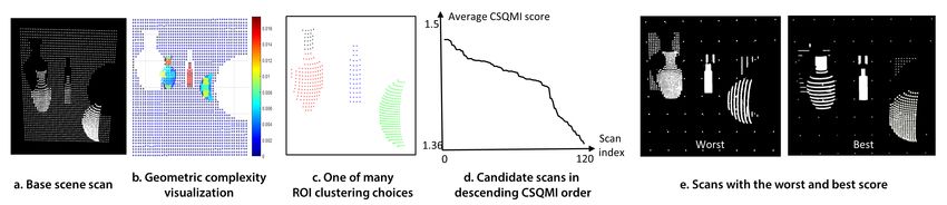
this paper, restricts us to static scenes. We prefer this LIDAR,
                                                                                    despite the low rate, since it allows for raw data capture, en-
                                                                                    abling design-specific calibration. We perform multiple scans
                                                                                    of the static scene, averaging our measurements to improve
                                                                                    accuracy. After the calibration in Fig 2(II) we reconstruct a
                                                                                    plane at 27cm (not in our calibration set) and obtained standard
                                                                                    deviation is 0.61cm (i.e. almost all points are measured in a
                                                                                    ±1.5cm error range), as shown in Fig 2(III).
                                                                                       The total weight of our system is approximately 500g;
                                                                                    however most of that weight ( 350g) is contained in a general
                                                                                    purpose oscilloscope and MEMS controller, and it would be
                                                                                    trivial to replace these with simple, dedicated circuits (67g
                                                                                    Lidar, 187g oscilloscope, 74g enclosure, 10g optics and 147g
                                                                                    MEMS controller).

                                                                                    B. Directional control of TOF sensing
                                                                                       Voltages over the MEMS device’s range physically shift
                                                                                    the mirror position to a desired angle, allowing for range
                                                                                    sensing over the direction corresponding to this angle. Let the
                                                                                    function controlling the azimuth be φ(V (t)) and the function
                                                                                    controlling elevation be θ(V (t)), where V is the input voltage
                                                                                    that varies with time t. W.l.o.g, we assume a pulse-based
                                                                                    system, and let the firing rate of the LIDAR/TOF engine be
                                                                                     1                                                           th
                                                                                    Tf HZ, or Tf seconds between each pulse. Therefore, the n
                                                                                    measurement of the sensor happens along the ray direction
                                                                                    given by the angles (θ(V (n Tf )), φ(V (n Tf ))).
                                                                                       The world around a miniature vision sensor can be mod-
                                                                                    eled as a hemisphere of directions (Fig 1(I) center), i.e. the
                                                                                    plenoptic function around the sensor is an environment map
                                                                                    parameterized by the azimuth and elevation angles. Just as
                                                                                    conventional imagers are characterized by their point-spread
                                                                                    function (PSF [9]), miniature vision systems are characterized
                                                                                    by their angular support ω [21]. For miniature active scanning
                                                                                    TOF systems, the angular spread of the laser beam determines
Fig. 2. Calibration: In (I) we show a screenshot of the voltages that control the   the angular support, which we term as ωlaser in Fig 1.
MEMS mirror pose, as well as an example of the return pulse. We fit a fourth-
order polynomial to the return pulse to detect the extrema location. In (II) we
show how to map this extrema location to depth in cm, by collecting data            C. Deblurring TOF measurements over the FOV
across five planes at known depths. This calibration also involves a vignetting
step, to remove effects in the the receiver optics. In (III) we validate our
                                                                                       Each sensor measurement occurs across the laser’s dot size,
sensor by reconstructing a fronto-parallel plane at 27cm, showing a standard        given by the angular support ωlaser . Let us now define the
deviation of 0.61cm (i.e. almost all points are measured in a ±1.5cm error          separation between measurements in angular terms, as ωdif f .
range). In the current configuration, the FOV is ≈ 15◦ and the range is 0.5m.
                                                                                    For many commercial LIDARs, such as the Velodyne HDL-
long wave IR (14 µm). As shown in Fig 2(I), voltages from                           32E, the measurement directions are further apart than the
an oscilloscope control the MEMS mirror direction, and the                          angular support; i.e. ωdif f ≥ ωlaser .
synchronized received pulses are inverted.                                             For our system, the measurement separation ωdif f de-
   The short focus lens introduces an interesting trade-off                         pends on the differential azimuth-elevation, given by ωdif f =
between FOV, range and accuracy. At the extreme case, with                          δφ δθ sin(φ), where φ and θ were defined previously.
no lens, our FOV reduces to a single receiving direction with                          MEMS-modulation allows almost any angle inside the sen-
the full range of the LIDAR (nearly 50m). As we increase the                        sor’s FOV. Therefore, if the measurements satisfy the inequal-
FOV, and the defocus, the SNR received at the transducer                            ity ωdif f ≤ ωlaser , then the measurements are correlated.
decreases, reducing range. While we can compensate with                                Therefore, we have defined the inequality that transforms
increased gain, this introduces noise and reduces accuracy. In                      our sensor into one identical to fixed resolution imagers. If
this paper, we traded-off range for accuracy and FOV, and our                       this inequality is satisfied, then the rich body of work in
device has a FOV of ≈ 15◦ , a range is 0.5m and is set at the                       vision using controllable PSFs can be applied here, including
lowest gain (highest SNR).                                                          image deblurring [36], refocussing [28], depth sensing [23]
   The Lightware LIDAR sampling rate is 32HZ, which, in                             and compressive sensing [7].
Fig. 3. Deblurring using angular support: In (I-III) we show simulations of pulse-based LIDAR with 2% noise on a simple 2D circular scene with a sharp
protrusion. In (Ia-b) the native laser dot size blurs the scene equiangularly, resulting in a banded matrix I(c) which is invertible I(d). In II (a-b) a larger angular
support is created with additional optics, for a sensor with non-uniform angular sampling. The matrix is still invertible, and can be used to resample the scene
uniformly II(c-d). (III) shows the effect of wide-angle optics, modeled from the refractive optics in [21, 43], where deblurring is still successful. Finally (IV)
shows real experiments across a depth edge. Without deblurring, depth measurements are hallucinated across the gap.
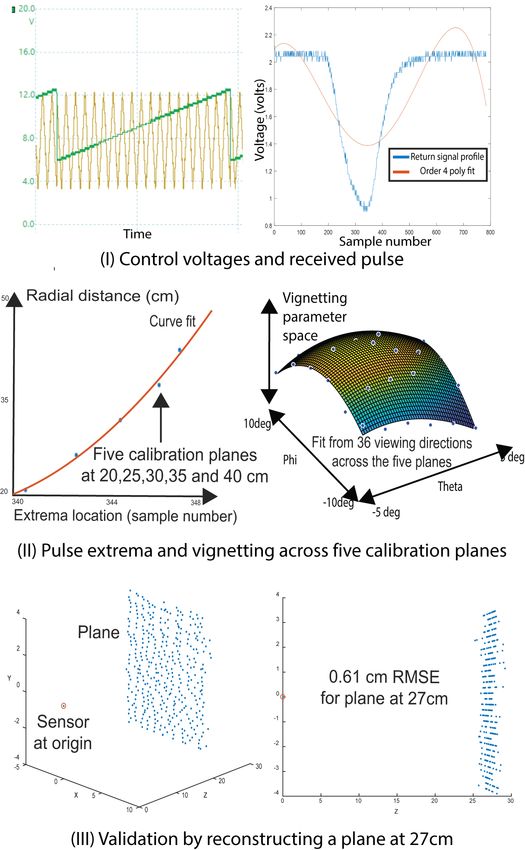
Fig. 4. Simulation of adaptive LIDAR: In (a) we show a base scan of a scene with three simple objects. This base scan is tesselated into boxes which are
scored according to some desired metric. In (b) we show a geometric score based on the residual of 2D principal component analysis of points in a box. Note
the background plane has a low score. This score is used with multiple values of cluster number k to generate many region-of-interest (ROI) segmentation,
as in (c). The ROIs globally direct the MEMS mirror to scan longer in regions with a higher average box score. For each ROI segmentation, many candidate
scans are generated by varying scan parameters such as phase, shape, directionality, etc, whose CSQMI scores are shown in (d). We show the highest and
lowest average CSQMI scores of these scans, and the highest scan’s MEMS mirror motions would be the actual trajectories scanned next.

   As an example, in Fig 3, we show noisy simulations of a                     such as a fish-eye lens. This would shear the diagonal band
2D toy scene where a MEMS modulated LIDAR is shown to                          in the matrix, where extreme angles would integrate large
be scanning a circular scene with a sharp discontinuity. The                   portions of the field of view, which samples closer to the
angular support ωlaser is shown to be much larger than the                     optical axis would show finer angular resolution. The smooth
differential measurement angle ωdif f , and therefore the direct               motion of the MEMS mirror allows us to invert or redistribute
measurements blur the high frequency information in the sharp                  the samples across the field-of-view, removing wide-angle
discontinuity in Fig 3 I(b).                                                   distortion. In Fig 3 III(c) we shown an example of such
   Assuming the intensity across the laser dot is uniform, we                  optics [21, 43] which has been used recently in wide-angle
can represent the angular support for any particular MEMS                      MEMS modulation. Using the equation from [21], we generate
mirror position as an indicator vector along viewing direction.                the viewing-dependent angular support that creates a blurred
We concatenate these binary indicator vectors across MEMS                      version of the scene in Fig 3 III(b) and a non-banded diagonal
mirror directions over the entire FOV to give a measurement                    matrix in Fig 3 III(c). This matrix is geometrically constructed
matrix B shown in Fig 3 I(c). In Fig 3 I(c), the rows of the                   to be invertible since all its values as positive and its trace is
matrix B are the indices of different measurements, and the                    non-zero, and allows for recovery of the scene in Fig 3 III(d).
columns cover discrete viewing directions across the FOV. Any                     In Fig. 3 (IV) we show a real deblurring result. The scene is
measurement collects information across the angular support                    two planes at 27cm and 30cm, where the sensing angles follow
in this FOV, given as white, and ignores the rest, shown as                    a great arc in the hemisphere of directions, as shown by the
black.                                                                         line segment in Fig. 3 (IV)a. We measure the angular support
   Therefore the measured, received pulses at the sensor are                   ωlaser as 0.9◦ as shown in Fig. 3 (IV)b. Without deblurring,
given y = Bz, where z is a vector of the ground-truth received                 the original measurements result in a smoothed edge, as shown
pulses for an ideal angular support ωlaser . Recovering the z is               in Fig. 3 (IV)c-d in blue. We use the damped Richardson-
a deblurring problem and we apply non-negative least squares                   Lucy blind deconvolution optimization algorithm that takes
to obtain measurements as shown in Fig 3 I(d), with zero                       our measured angular support as a starting point, as shown in
RMSE error.                                                                    Fig. 3 (IV)c. This results in a strong edge recovery, with fewer
   We note that the angular support of the sensor is constant                  incorrect measurements, as shown in red in Fig. 3 (IV)c-d.
across viewing direction, because it is simply the angular
spread of the laser being reflected off the MEMS mirror. This                  D. Adaptive TOF sensing in selected ROIs
results in a near-perfect banded diagonal matrix in Fig 3 I(c),                   The MEMS mirror can modulate the LIDAR beam through
which is invertible. The angular spread can be affected by                     a range of smooth trajectories. A unique characteristic of our
adding laser optics, as shown in Fig 3 (II)a, where the angular                setup is that we can adapt this motion to the current set
support ωlaser is increased.                                                   of scene measurements. We control the MEMS mirror over
   This would be necessary if the maximum angular spread                       the FOV by exploiting strategies used for LIDAR sensing
between measurements is much larger than the original angular                  in robotics [18, 5, 40]. In particular, we first generate a
support ωlaser , due to non-uniform MEMS mirror control. In                    series of candidate trajectories that conform to any desired
fact, such control occurs naturally with MEMS devices driven                   global physical constraints on the sensor. We then select from
by linear signals, since the MEMS device’s forces follow                       these candidates by maximizing a local information theoretic
Hooke’s law of springs [44]. In Fig 3 II(c) the non-uniform and                measure that has had success in active vision for robotics [5].
blurred measurements result in a banded matrix with varying                       Candidate trajectories from global physical constraints
band-width. The ground-truth recovered is both accurate and                    To generate a series of candidate trajectories, we encode the
with the desired uniform density sampling.                                     scene into regions where the sensing beam should spend more
   Finally, consider the effect of a wide-angle optical system,                time collecting many measurements, and regions where the
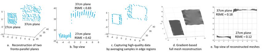
Fig. 5. Our smart LIDAR zoom vs. naive LIDAR zoom: By moving the MEMS mirror to certain regions of interest, we can “zoom” or capture more angular
resolution in that desired region. In (a) we show a scene with two objects, and in (b) we show the output of our sensor with equiangular sampling. If the
zoom shifts to the flower, then the naive zoom concentrates the samples in the base scan on the flower exclusively, in (c). On the other hand, our smart zoom
(d) takes measurements outside the zoom region, depending on neighboring object’s complexity and proximity. A naive approach does not visually support
scrolling, since other areas of the scene are blank (e). Our smart zoom allows for scrolling to nearby objects that have some measurements (f). This allows a
for smoother transition when the zoom shifts to that object (g), when compared to the naive zoom.

beam should move quickly, collecting fewer measurements.                        is a user defined weight that controls the impact of the relative
We achieve this by clustering the scene into regions of interest                score of the different ROIs on the time spent in each ROI. If
(ROI) based on a desired physical metric. In the applications                   mtotal = Σkj mj , we pick a weight α such that the time spent
                                                                                                                   mj
section, we show that different metrics can enable, for exam-                   in each ROI is proportional to mtotal   .
ple, scanning the scene under the constraint of limited power.                     Note that the above equation does not contain a derivative
                                                                                        0
Similar metrics can be specified for time or scene complexity.                  term V (t) to enforce smoothness, since we generate only
   We first tessellate the current scene scan in three dimensions               candidate trajectories that conform to physically realizable
into bounding boxes Bi (Xc , Yc , Zc , H), which contain all                    MEMS mirror trajectories, such as sinusoids, triangular wave
points (X, Y, Z) in the current scan such that these lie in a                   functions and raster scans. We generate P such scans Vp (t)
box centered at (Xc , Yc , Zc ) with side length given by H. We                 and pick the scan that maximizes the sum of the information
require that a metric M be designed such that M (Bi ) ∈ R.                      gain from each scanned ray
We then apply an unsupervised clustering mechanism, such as
k-means, to the set of boxes, where the feature to be clustered                                               max I(m|xt )                               (2)
                                                                                                             Vp (t),m
from each box Bi is (M (Bi ), Xc , Yc , Zc ). Automatically
finding the number of clusters is an open problem in pattern                    where xt is the current scan and m is the probabilistic occu-
recognition, and while a variety of methods exist to find an                    pancy map of the scene calculated by tessellating the scene
                                                                                               0  0    0   0    0
optimal k, for simplicity we generate candidate trajectories                    into voxels Bi (Xc , Yc , Zc , H ), and where the probability of
over a range of cluster centers, from 2 till kmax , which we                    occupancy is given by e−0.5r , where r is the radial distance
leave as a design parameter.                                                    between the voxel center and the nearest measured scan point.
   Each cluster of boxes defines a region of interest (ROI) in                     We use a form for I(m|xt ) in Eq 2 derived from the
the scene. Let us describe the solid angle subtended by the                     Cauchy-Schwarz quadratic mutual information (CSQMI) for
ROI onto the MEMS mirror, indexed by j as ωj , and let the                      a single laser beam [5]. The expression for CSQMI is repro-
average metric of all the boxes in the j th ROI be mj . If there                duced here from [5],
are n samples across the FOV, then our goal is to create a series
of voltages V (t), such that the angles generated maximize the                   log ΣC              2
                                                                                      l=0 wl N (0, 2σ )
following cost function,                                                         + log ΠC     2            2  C    C                              2
                                                                                        i=1 (oi + (1 − oi ) )Σj=0 Σl=0 p(ej )p(el )N (µl − µj , 2σ )

                                                                                 − 2 log ΣC    C                           2
                                                                                          j=0 Σl=0 p(ej )wl N (µl − µj , 2σ )
           (n Tf )                                                                                                                                       (3)
   max Σi            Σkj F (θ(V (n Tf )), φ(V (n Tf )), ωj , mj ),       (1)
   V (t)
                                                                                where C refers to the number of “cells” — voxels intersected
where k is the number of ROI clusters in that scan, T1f is the                  by the current laser ray direction, N and σ define the mean
firing of the LIDAR/TOF engine and where F is a function                        and variance of a Gaussian model of the return pulse, oi
that outputs eαmk if (θ(V (n Tf )), φ(V (n Tf )) lie inside ωk . α              is the probability that the ith cell is occupied, p(ej ) is the
probability that the j th cell is the first occupied cells (with
all before being unoccupied) and wl is a weight defined by
wl = p2 (el )ΠC 2 2
j=l+1 (oj +(1−oj ) ). Since we have multiple ray
directions in each candidate scan, we aggregate each of these
to produce a single, overall CSQMI value for that candidate
scan and pick the scan with the maximum score.
Simulation example In Fig 4 we show a scene created with
BlenSor [10] with three objects in front of a fronto-parallel
plane. We start with a equi-angular base scan shown in Fig
4(a) since all directions have uniform prior. We tesselate the
scene into boxes B of size 25cm × 25cm × 25cm and use
the residuals of a 2D principal component analysis fit to score
the complexity of each box, as in Fig 4(b). Clustering the
boxes Fig 4(c) creates regions of interest. Varying the number
of clusters and varying scan parameters creates a variety of
candidate, each of which have a CSQMI score Fig 4(d). We
pick the best such score, as shown in Fig 4(e), where it is
contrasted with the worst such scan. Note that, in the best
scan, the neck of the vase is captured in detail and the sphere
is captured equally densely across θ and φ angles.
IV. A PPLICATIONS
The imaging framework we have just described allows for
Fig. 6. Energy aware adaptive sampling: We augment our directional control
directional control of TOF measurements. Using these ideas algorithm for adaptive TOF with physical constraints that capture the energy
and our MEMS mirror-based LIDAR sensor, we demonstrate budget of the system. Here we use two constraints; the inverse fall-off of
the following novel applications. light beam intensity and the motion of scene objects w.r.t to the sensor FOV.
In (a) we show simulations of three objects, one of which is give a motion
perpendicular to the optical axis (i.e. leaving the sensor FOV cone). Compared
A. Smart LIDAR zoom to the base scan (left), the effiency scan reduces sampling on objects that move
beyond the FOV cone and distant objects, despite their complexity. In (b) we
Optical zoom with a conventional fixed array of detectors show a real example using our MEMS mirror-based sensor, where, again,
involves changing the field-of-view so that the measurements distant objects are subsampled.
are closer together in the angular domain. The key component In Fig 5(a) we show a scene with a 3D printed flower
of zoom is that new measurements are made, when compared and a bottle. We show a base scan of the scene in Fig 5(b)
to the initial image. with equiangular samples. The user places a zoom region of
Intelligent zoom exists for conventional cameras using pan- interest around the flower. We show that naive zoom directs
zoom-tilt transformations [6] and light-fields [2]. Here we the measurements entirely on the flower, with almost zero
demonstrate, for the first time, intelligent LIDAR zoom. measurements around the zoomed-in area.
Suppose we are provided with angular supports While we have not implemented real-time scrolling, in Fig
of n interesting regions of interest in the scene 5(c-g) we simulate the effect of scroll in naive zoom, showing
1 2 n
(ωzoom , ωzoom , ...ωzoom ) and a corresponding series of a jarring transition period in the image, since the measure-
importance weights (w1 , w2 , ..., wn ). These could come from ments suddenly appear in a previously blank image. Instead,
another algorithm, say face detection, or from a user giving our method spreads the samples across the two complex
high-level commands to the system. objects in the scene, allowing for a more meaningful transition
We can use these regions and weights to modify the default when scrolling is simulated in Fig 5(g) to the dense scan when
effect of the adaptive LIDAR framework described in Sect the bottle is zoomed. Note, that while the scroll motion is
i
III-D. For example, if a box is contained in ωzoom , then we simulated, all the zoom measurements are real measurements
can increase the geometric score in the boxes by a factor from our sensor performing directionally varying sampling,
determined by the corresponding importance weight wi . This based on the desired zoom area.
would increase the amount of time that the sensor spends in
the angular support corresponding to the box. B. Energy-aware adaptive sampling
Smart LIDAR zoom has a clear advantage over naive zoom, In its current form, the adaptive TOF sensing algorithm only
which would place all LIDAR samples exclusively in ROIs. uses a geometric goodness metric. To augment the algorithm
This because any zoom interface must also offer scrolling. As for mobile-based platforms, we wish to include multiple, say
is known in computer graphics [27], efficient scrolling requires n, physical constraints into the metric. Therefore we redefine
caching motion and data near user viewpoints, to allow for fast the metric as M (Bi ) ∈ Rn , where Bi is the ith box in the
rendering for real-time interaction. tessellated current scan.Fig. 7. Gradient-based reconstruction: Directional control allows a capture of the scene, where samples are only made in high-frequency (i.e. edge) regions
of the scene. In (a) we see the original scan of the two planes, and (b) illustrates their noise levels. In (c), we directly capture only edge regions, placing the
same number of samples as in (a) in high-frequency areas, improving averaging and reducing error. We use these edges with a gradient-based reconstruction
algorithm to recover the meshes in (d). Note that the noise levels are significantly reduced, as shown in (e).
To illustrate the redefined metric, we point out differences
between adaptive sensing when compared to adaptive sampling
literature in image processing and graphics. First, for a given
pulse signal and desired SNR, distant objects require more
pulses. Therefore, geometric complexity must trade-off with
range, and a distant, intricate object may not be sampled
at the required resolution, to save energy. Second, temporal
relevance matters, and a nearby, intricate object that is rapidly Fig. 8. In (I) we depict the deblurring trade-off in our setup, where increasing
moving out of the field-of-view need not be sampled at high FOV results in reduced SNR and range. In (II) we compare our LIDAR zoom
resolution. Third, unlike virtual scenes, free space must be to other available depth sensors which have fixed acuity.
sampled periodically, since new obstacles may emerge. Finally, and y gradients. Formulating this for our scenario,
the sensor’s measurement rate, implies finite samples which
must be shared across all objects, complex or simple. dẐ dZ 2 dẐ dZ 2
min k − k +k − k . (4)
The issues of free space and infinite samples are already Z dx dx dy dy
handled by the adaptive algorithm described in Sect III-D, and Note that the minimization estimates scene depth Z, which
we augment it with two new metrics in M (Bi ). The first takes has values outside the sparse locations where we have mea-
into account the dissipation of the laser, and scores distant surements; i.e. it is a full scene reconstruction. In Fig. 7
objects by two-way inverse square reduction in radiance, or we show a real example of gradient-based reconstruction for
1
Z 4 . The second is simply a scaled version of the object’s a scene with two planes at 27cm and 37cm. We captured
velocity λ~v , where λ is 1 if the direction ~v is contained in the a base scan in Fig. 7(a) of the scene and, using its depth
FOV cone of the sensor, and zero otherwise. gradients, captured a new set of measurements along edges
Fig. 6 shows both simulated and real scenes, where objects Fig. 7(b). These were used with a widely available gradient
are at different distances from the sensor. In the simulated reconstruction method [13] which reduced the corresponding
scene, the vase is given a motion away from the sensor’s RSME errors in Fig. 7(e) by a third.
visual cone. In the first column we see the base scan of the
scene, where samples are taken equiangularly. Applying the V. L IMITATIONS AND C ONCLUSION
physical restrictions discussed above and using the adaptive Although we show only static scene reconstructions, our
algorithm described in Sect III-D produces the results in the adaptive angular framework impacts any scanning TOF sensor.
second column, where samples are reduced to save energy Deblurring tradeoff: Given a minimum, required incident
consumption and time. radiance at the photodetector, our sensor range Z and field-
of-view Θ are inversely proportional, Z 2 ∝ tan(1 Θ ) (Fig.
2
C. Edge sensing for gradient-based reconstruction 8(I)). Our results have significant scope for improvement in
measurement SNR of the reconstructions, and we will focus
Gradient-based methods [31] have had significant impact in on better optical designs in the future.
vision, graphics and imaging. Given a base scan of the scene, System performance: In Fig. 8(II), we compare the ability
we can focus our sensor to place samples only on regions of to induce desired sample density on targets. For conventional
high-frequency changes in depth. Placing all our samples in sensors, as the density increases, the robot-target distance goes
these regions, over the same time it took to previously scan to zero. For our sensor design, a stand-off distance is possible
the entire scene, produces more robust data since averaging since we can concentrate samples on the target.
can reduce noise in these edge regions. Efficiency/power reduction applications: We will use
Our goal is to estimate scene depths Z, from a small number energy efficient adaptive sensing for UAVs and other power
of captured depths Ẑ. A popular solution is to minimize some constrained robots to place the samples on nearby obstacles
norm between the numerically computed real and estimated x and targets, accruing power savings.R EFERENCES 33(9):1271–1287, 2014.
[16] Shahram Izadi, David Kim, Otmar Hilliges, David
[1] Supreeth Achar, Joseph R Bartels, William L Whittaker, Molyneaux, Richard Newcombe, Pushmeet Kohli, Jamie
Kiriakos N Kutulakos, and Srinivasa G Narasimhan. Shotton, Steve Hodges, Dustin Freeman, Andrew Davi-
Epipolar time-of-flight imaging. ACM Transactions on son, et al. Kinectfusion: real-time 3d reconstruction and
Graphics (TOG), 36(4):37, 2017. interaction using a moving depth camera. In Proceedings
[2] Abhishek Badki, Orazio Gallo, Jan Kautz, and Pradeep of the 24th annual ACM symposium on User interface
Sen. Computational zoom: a framework for post-capture software and technology, pages 559–568. ACM, 2011.
image composition. ACM Transactions on Graphics [17] A. Jones, I. McDowall, H. Yamada, M. Bolas, and
(TOG), 36(4):46, 2017. P. Debevec. Rendering for an interactive 360 degree light
[3] Jacques M Beckers. Adaptive optics for astronomy: field display. In SIGGRAPH. ACM, 2007.
principles, performance, and applications. Annual review [18] Brian J Julian, Sertac Karaman, and Daniela Rus. On
of astronomy and astrophysics, 31(1):13–62, 1993. mutual information-based control of range sensing robots
[4] Alvin T Campbell III and Donald S Fussell. Adaptive for mapping applications. The International Journal of
mesh generation for global diffuse illumination. In ACM Robotics Research, 33(10):1375–1392, 2014.
SIGGRAPH Computer Graphics, volume 24, pages 155– [19] Abhishek Kasturi, Veljko Milanovic, Bryan H Atwood,
164. ACM, 1990. and James Yang. Uav-borne lidar with mems mirror-
[5] Benjamin Charrow, Gregory Kahn, Sachin Patil, Sikang based scanning capability. In Proc. SPIE, volume 9832,
Liu, Ken Goldberg, Pieter Abbeel, Nathan Michael, and page 98320M, 2016.
Vijay Kumar. Information-theoretic planning with tra- [20] Sanjeev J Koppal, Shuntaro Yamazaki, and Srinivasa G
jectory optimization for dense 3d mapping. In Robotics: Narasimhan. Exploiting dlp illumination dithering for
Science and Systems, 2015. reconstruction and photography of high-speed scenes.
[6] Thomas Deselaers, Philippe Dreuw, and Hermann Ney. International journal of computer vision, 96(1):125–144,
Pan, zoom, scantime-coherent, trained automatic video 2012.
cropping. In Computer Vision and Pattern Recognition, [21] Sanjeev J Koppal, Ioannis Gkioulekas, Travis Young,
2008. CVPR 2008. IEEE Conference on, pages 1–8. Hyunsung Park, Kenneth B Crozier, Geoffrey L Barrows,
IEEE, 2008. and Todd Zickler. Toward wide-angle microvision sen-
[7] Rob Fergus, Antonio Torralba, and William T Freeman. sors. IEEE Transactions on Pattern Analysis & Machine
Random lens imaging. 2006. Intelligence, (12):2982–2996, 2013.
[8] Thomas P Flatley. Spacecube: A family of reconfigurable [22] Krassimir T Krastev, Hendrikus WLAM Van Lierop,
hybrid on-board science data processors. 2015. Herman MJ Soemers, Renatus Hendricus Maria Sanders,
[9] Joseph W Goodman et al. Introduction to Fourier optics, and Antonius Johannes Maria Nellissen. Mems scanning
volume 2. McGraw-hill New York, 1968. micromirror, September 3 2013. US Patent 8,526,089.
[10] Michael Gschwandtner, Roland Kwitt, Andreas Uhl, and [23] Anat Levin, Rob Fergus, Frédo Durand, and William T
Wolfgang Pree. Blensor: blender sensor simulation tool- Freeman. Image and depth from a conventional camera
box. In International Symposium on Visual Computing, with a coded aperture. In ACM Transactions on Graphics
pages 199–208. Springer, 2011. (TOG), volume 26, page 70. ACM, 2007.
[11] Mohit Gupta, Shree K Nayar, Matthias B Hullin, and [24] V Milanović, A Kasturi, N Siu, M Radojičić, and Y Su.
Jaime Martin. Phasor imaging: A generalization of memseye for optical 3d tracking and imaging applica-
correlation-based time-of-flight imaging. ACM Transac- tions. In Solid-State Sensors, Actuators and Microsystems
tions on Graphics (ToG), 34(5):156, 2015. Conference (TRANSDUCERS), 2011 16th International,
[12] Ryan Halterman and Michael Bruch. Velodyne hdl- pages 1895–1898. IEEE, 2011.
64e lidar for unmanned surface vehicle obstacle detec- [25] Veljko Milanović, Abhishek Kasturi, James Yang, and
tion. Technical report, SPACE AND NAVAL WARFARE Frank Hu. A fast single-pixel laser imager for vr/ar
SYSTEMS CENTER SAN DIEGO CA, 2010. headset tracking. In Proc. of SPIE Vol, volume 10116,
[13] Matthew Harker and Paul OLeary. Regularized recon- pages 101160E–1, 2017.
struction of a surface from its measured gradient field. [26] Shree K Nayar, Vlad Branzoi, and Terry E Boult. Pro-
Journal of Mathematical Imaging and Vision, 51(1):46– grammable imaging: Towards a flexible camera. Inter-
70, 2015. national Journal of Computer Vision, 70(1):7–22, 2006.
[14] Felix Heide, Matthias B Hullin, James Gregson, and [27] Diego Nehab, Pedro V Sander, and John R Isidoro. The
Wolfgang Heidrich. Low-budget transient imaging using real-time reprojection cache. In ACM SIGGRAPH 2006
photonic mixer devices. ACM Transactions on Graphics Sketches, page 185. ACM, 2006.
(ToG), 32(4):45, 2013. [28] Ren Ng. Fourier slice photography. In ACM Transactions
[15] Geoffrey A Hollinger and Gaurav S Sukhatme. on Graphics (TOG), volume 24, pages 735–744. ACM,
Sampling-based robotic information gathering algo- 2005.
rithms. The International Journal of Robotics Research, [29] Matthew O’Toole, Felix Heide, Lei Xiao, Matthias BHullin, Wolfgang Heidrich, and Kiriakos N Kutulakos. Moungi Bawendi, Diego Gutierrez, and Ramesh Raskar.
Temporal frequency probing for 5d transient analysis of Imaging the propagation of light through scenes at pi-
global light transport. ACM Transactions on Graphics cosecond resolution. Communications of the ACM, 59
(ToG), 33(4):87, 2014. (9):79–86, 2016.
[30] Matthew O’Toole, Supreeth Achar, Srinivasa G [43] B Yang, L Zhou, X Zhang, S Koppal, and H Xie. A com-
Narasimhan, and Kiriakos N Kutulakos. Homogeneous pact mems-based wide-angle optical scanner. In Optical
codes for energy-efficient illumination and imaging. MEMS and Nanophotonics (OMN), 2017 International
ACM Transactions on Graphics (ToG), 34(4):35, 2015. Conference on, pages 1–2. IEEE, 2017.
[31] Patrick Pérez, Michel Gangnet, and Andrew Blake. Pois- [44] Hao Yang, Lei Xi, Sean Samuelson, Huikai Xie, Lily
son image editing. ACM Transactions on graphics Yang, and Huabei Jiang. Handheld miniature probe in-
(TOG), 22(3):313–318, 2003. tegrating diffuse optical tomography with photoacoustic
[32] Kurt E Petersen. Silicon torsional scanning mirror. IBM imaging through a mems scanning mirror. Biomedical
Journal of Research and Development, 24(5):631–637, optics express, 4(3):427–432, 2013.
1980.
[33] Christopher V Poulton, Ami Yaacobi, David B Cole,
Matthew J Byrd, Manan Raval, Diedrik Vermeulen, and
Michael R Watts. Coherent solid-state lidar with silicon
photonic optical phased arrays. Optics letters, 42(20):
4091–4094, 2017.
[34] Jose C Principe, Neil R Euliano, and W Curt Lefebvre.
Neural and adaptive systems: fundamentals through sim-
ulations, volume 672. Wiley New York, 2000.
[35] Ramesh Raskar, Greg Welch, Matt Cutts, Adam Lake,
Lev Stesin, and Henry Fuchs. The office of the future: A
unified approach to image-based modeling and spatially
immersive displays. In Proceedings of the 25th annual
conference on Computer graphics and interactive tech-
niques, pages 179–188. ACM, 1998.
[36] Ramesh Raskar, Amit Agrawal, and Jack Tumblin.
Coded exposure photography: motion deblurring using
fluttered shutter. ACM Transactions on Graphics (TOG),
25(3):795–804, 2006.
[37] Thilo Sandner, Claudia Baulig, Thomas Grasshoff,
Michael Wildenhain, Markus Schwarzenberg, Hans-
Georg Dahlmann, and Stefan Schwarzer. Hybrid as-
sembled micro scanner array with large aperture and
their system integration for a 3d tof laser camera. In
MOEMS and Miniaturized Systems XIV, volume 9375,
page 937505. International Society for Optics and Pho-
tonics, 2015.
[38] Barry L Stann, Jeff F Dammann, Mark Del Giorno,
Charles DiBerardino, Mark M Giza, Michael A Powers,
and Nenad Uzunovic. Integration and demonstration of
mems–scanned ladar for robotic navigation. In Proc.
SPIE, volume 9084, page 90840J, 2014.
[39] Demetri Terzopoulos and Manuela Vasilescu. Sampling
and reconstruction with adaptive meshes. In Com-
puter Vision and Pattern Recognition, 1991. Proceedings
CVPR’91., IEEE Computer Society Conference on, pages
70–75. IEEE, 1991.
[40] Sebastian Thrun, Wolfram Burgard, and Dieter Fox.
Probabilistic robotics. MIT press, 2005.
[41] Robert K Tyson. Principles of adaptive optics. CRC
press, 2015.
[42] Andreas Velten, Di Wu, Belen Masia, Adrian Jarabo,
Christopher Barsi, Chinmaya Joshi, Everett Lawson,You can also read