LINQ: A Framework for Location-aware Indexing and Query Processing
←
→
Page content transcription
If your browser does not render page correctly, please read the page content below
This article has been accepted for publication in a future issue of this journal, but has not been fully edited. Content may change prior to final publication. Citation information: DOI
                                               10.1109/TKDE.2014.2365792, IEEE Transactions on Knowledge and Data Engineering
                                                                                                                                                                     1

                      LINQ: A Framework for Location-aware
                         Indexing and Query Processing
                                           Xiping Liu, Lei Chen, Member, IEEE, and Changxuan Wan

                 Abstract—This paper studies the generic location-aware rank query (GLRQ) over a set of location-aware objects. A GLRQ is
                 composed of a spatial location, a set of keywords, a query predicate, and a ranking function formulated on location, text and
                 other attributes. The result consists of k objects satisfying the predicate ranked according to the ranking function. An example
                 is a query searching for the restaurants that 1) are nearby, 2) offer “American” food, and 3) have high ratings (rating > 4.0).
                 Such queries can not be processed efficiently using existing techniques. In this work, we propose a novel framework called LINQ
                 for efficient processing of GLRQs. To handle the predicate and the attribute-based scoring, we devise a new index structure
                 called synopses tree, which contains the synopses of different subsets of the dataset. The synopses tree enables pruning of
                 search space according to the satisfiability of the predicate. To process the query constraints over the location and keywords,
                 the framework integrates the synopses tree with the spatio-textual index such as IR-tree. The framework therefore is capable of
                 processing the GLRQs efficiently and holistically. We conduct extensive experiments to demonstrate that our solution provides
                 excellent query performance.

                 Index Terms—Location-aware, rank query, synopses tree, LINQ

                                                                                       F

          1     I NTRODUCTION
          With the proliferation and widespread adoption of
          mobile telephony, it is more and more convenient
          for users to capture and publish geo-locations. As a
          consequence, more and more location-aware datasets
          have been created and made available on the Web.
          For example, Flickr, one of the biggest photo-sharing
          website, has millions of geo-tagged items every month
          1
            . The popularity and large scale of the location-aware
          datasets make location-aware queries important.                                  Fig. 1. A snippet about a restaurant on Yelp.com
              In this work, we are interested in location-aware
          rank query, an important class of location-aware
          query. Examples of location-aware rank query include                             of reviews (150). Another example is the photos on
          the (k-) nearest neighbor (NN) query and location-                               Flickr, where in addition to the geo-location and text,
          aware keyword query (LKQ, a.k.a spatial keyword                                  each photo also has some numeric attributes, such
          query) [1], [2], [3], [4], [5] and [6]. NN queries and                           as the number of views, the number of favorites, the
          LKQs have wide applications in many domains. How-                                number of comments, and so on. The restaurants on
          ever, there are a lot of location-aware datasets that                            Yelp and photos on Flickr are mixtures of location,
          demand more powerful and flexible location-aware                                 text and other types of information. They are much
          rank queries. Fig. 1 shows an example of a restaurant                            more complex than spatio-textual objects. We term
          on Yelp 2 . For the restaurant, Yelp gives its location                          these objects as location-aware objects. For location-
          (“1429 Mendell St, San Francisco, CA 94124”), cat-                               aware objects, simple NN queries and LKQs may not
          egories (“Soul Food, American (Traditional), Music                               be expressive enough to find the objects of interests.
          Venues”), rating (4.5 stars) as well as the number                               For example, on the restaurant dataset, through LKQs,
                                                                                           one can find the most nearest and relevant restaurants.
          • Xiping Liu and Changxuan Wan are with the Jiangxi University of                But one may hope to find the nearest and relevant
            Finance and Economics, Nanchang 330013, China. E-mail: lewislxp@               restaurants satisfying certain conditions, such as no-
            gmail.com, wanchangxuan@263.net
                                                                                           smoking, healthy, or top-ranked. On the Flickr dataset,
          • Lei Chen is with the Department of Computer Science and Engineering,           users may want to fetch the relevant and nearest
            The Hong Kong University of Science and Technology, Clear Water                photos that are highly-rated. On these datasets, people
            Bay, Kowloon, Hong Kong, China. E-mail: leichen@cse.ust.hk.
                                                                                           may wish to search by not only location and key-
              1. http://www.flickr.com/map/
                                                                                           words, but also conditions on other attributes.
              2. http://www.yelp.com                                                          In this paper, we study the generic location-aware

                                 1041-4347 (c) 2013 IEEE. Personal use is permitted, but republication/redistribution requires IEEE permission. See
                                         http://www.ieee.org/publications_standards/publications/rights/index.html for more information.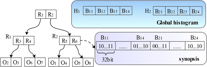
This article has been accepted for publication in a future issue of this journal, but has not been fully edited. Content may change prior to final publication. Citation information: DOI
10.1109/TKDE.2014.2365792, IEEE Transactions on Knowledge and Data Engineering
2
rank query (GLRQ) over a set of location-aware objects. first does even worse, because a top LKQ result, even
A GLRQ is composed of a query location, a set of satisfying the query predicate, may not be a top result
keywords, a query predicate, and a ranking function of Q2 . As for query Q3 , existing LKQ techniques do
combining spatial proximity, textual relevance and not help at all, because it does not contain keywords.
other measures (e.g. certain attribute values). The Although RDBMS can process Q2 and Q3 , as analyzed
result of the query consists of k objects that satisfy the before, the efficiency is very low.
predicate, ranked according to the specified ranking In this paper, we propose a novel framework,
function. Obviously, the GLRQ has the NN query and called LINQ (Location-aware INdex and Querying
LKQ as special cases. framework), to efficiently process the GLRQ. A core
Example 1: An example (Q1 ) of the GLRQ is to component of the framework is a new index structure
search restaurants near a certain location (denoted by called synopses tree, which stores synopses of different
loc) that provide “American traditional” food with sets of objects in a tree. The synopses tree can be com-
the constraint that the ratings should be above 4.0, bined with spatial index, e.g. R-tree, text index, e.g.
and rank the restaurants based on spatial proximities inverted file, or spatio-textual index, e.g. IR-tree [2], to
and textual relevances. The query intent cannot be ex- provide integrated indexing and querying capability.
pressed by a LKQ, because the predicate rating > 4.0 Based on the LINQ framework, we present the search
cannot be processed by simple keyword matching. If algorithm, especially estimation algorithm, for GLRQ.
we change the ranking function to consider also the In summary, we make the following contributions
ratings of objects, we get another query Q2 , which is in this paper:
also a GLRQ. Another example query (Q3 ) requests • We formulate the generic location-aware rank
hotels that are near a location and have popularities query (GLRQ), which retrieves the objects satis-
above 8.5. We can see that a GLRQ allows users fying a query predicate, ranks and returns the
to specify preferences on spatial, text and other at- results based on spatial proximity, textual rel-
tributes, thus is more powerful and flexible than NN evances and measures obtained from attribute
query and LKQ. We believe that this query will be values.
very helpful for users in many applications. • We develop a novel framework called LINQ, for
Up to now, we have not found any work devoted efficient indexing and querying of GLRQs. LINQ
to the generic form of location-aware rank query. One develops the synopses tree to utilize synopses of
may think that the GLRQs can be simply processed non-spatial attributes, and combines the synopses
based on the existing techniques. However, that is tree with other indexes to index and query the
not the case. Consider again the query Q1 shown in GLRQ.
Example 1. A straightforward approach to process • We conduct extensive experiments on both real
the query is as follows: incrementally compute the and synthetic datasets, and the results demon-
results of a LKQ Q0 (loc, “American traditional”) using strate the effectiveness and efficiency of our
existing techniques, then validate each object obtained method.
against the predicate (rating > 4.0), and finally return The rest of the paper is organized as follows. Sec-
the objects satisfying the predicate in a ranked order. tion 2 formally defines the problem. Section 3 intro-
In this approach (called LKQ-first approach), to get duces several possible solutions. Section 4 presents
top-k results, it is unavoidable to compute much more the LINQ framework. Empirical performances of our
intermediate results than k. For example, suppose proposal are evaluated in Section 5, and related work
only 1% restaurants have ratings above 4.0, and the is discussed in Section 6. Finally, we conclude the
query requests 3 results. Then the probability of ob- work in Section 7.
taining 3 final results after generating even 100 LKQ
results is still 0.0794 (more analyses will be presented
later). Another possible approach is to put everything 2 P ROBLEM S TATEMENT
in a relational database, and process the query within We denote a location-aware object O as a triple
RDBMS. In this approach, RDBMS will first obtain (λ, W, A), where O.λ is a location descriptor, O.W
all the candidates satisfying the predicate, and then is a set of keywords, and O.A = (O.A1 , O.A2 , · · · ) is
score the candidates. We assume the selectivity of the a set of attributes. We use O.Ai to denote the value
query predicate is ρ, and a secondary index (B+ -tree) of O on attribute Ai . Without loss of generality, we
has been built on the attribute rating. Then, the cost assume the attributes in O.A are numeric attributes.
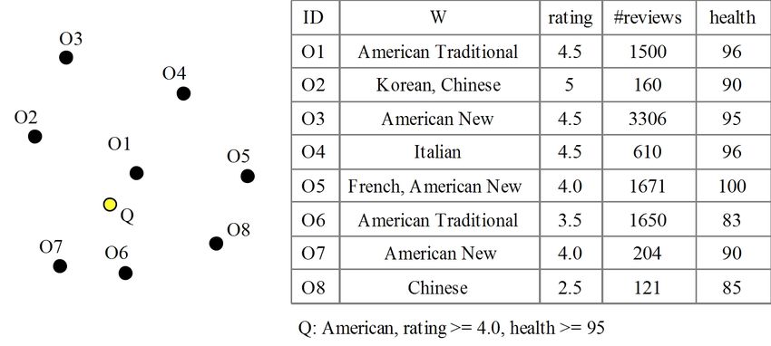
(in terms of number of disk access) of this approach Example 2: We use a dataset about restaurants as
is about HT + LB ∗ ρ + nr ∗ ρ [7], where HT is the an example throughout this paper. In this dataset, A
height of the B+ -tree, LB is the number of leaf blocks = (rating, #reviews, health), denoting the rating, the
in the index, and nr is the total number of objects. As number of reviews, and the health score of the restau-
nr can be a very large number, the cost is very high. rant, respectively. All these attributes are borrowed
Therefore, RDBMS cannot provide satisfactory query from Yelp. Fig. 2 shows several instances of object. The
performance. For the query Q2 in Example 1, LKQ- locations of the objects are implied by their positions
1041-4347 (c) 2013 IEEE. Personal use is permitted, but republication/redistribution requires IEEE permission. See
http://www.ieee.org/publications_standards/publications/rights/index.html for more information.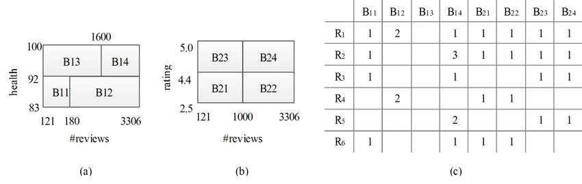
This article has been accepted for publication in a future issue of this journal, but has not been fully edited. Content may change prior to final publication. Citation information: DOI
10.1109/TKDE.2014.2365792, IEEE Transactions on Knowledge and Data Engineering
3
TABLE 1
Notations
Symbol Meaning
O = (λ, W, A) an object O described by a location λ, a set W
of keywords , and a set A of attributes
Q = (λ, W, P, f, k) a query Q described by a location λ, a set W
of keywords, a query predicate P , a ranking
function f , and the number k of results
N ( or e) a node (or an entry) in the synopses tree
N.syn (or e.syn) the synopses corresponding to N or e
Fig. 2. A set of location-aware objects N.D (or e.D) the dataset corresponding to N (or e)
Q(N ) the result of evaluating Q.P on N
H = {H1 , H2 , · · · } H is a set consisting of global histograms
H1 , H2 , · · ·
on the plane, and the attributes and keywords are Bij a bucket in the histogram Hi
shown in the table. B the set of global buckets, with cardinality |B|,
consisting of all buckets from the global his-
In this work, we are interested in a type of query, tograms
called generic location-aware rank query (GLRQ), which
allows users to specify constraints on spatial, text and
other attributes, and returns top-k results according to “otherwise” case) is defined as
user-provided ranking function.
Formally, a GLRQ Q is a quintuple (λ, W, P, f, k), f (O, Q) =w1 · prox(O, Q) + w2 · rel(O, Q)+
where Q.λ is the location descriptor of Q, and Q.W O.rating O.health
w3 · + w4 ·
is a set of keywords. Q.P is a query predicate of the 5.0 100
form P1 ∧ P2 ∧ · · · ∧ Pn , where Pi is a simple selection where w1 + w2 + w3 + w4 = 1. The query object is
predicate specified on a single attribute. The fourth depicted in yellow and other objects are depicted in
component Q.f is a ranking function. We assume each black in Fig. 2. The results of the query should be O1 ,
attribute, including location and text, has a scoring O5 and O3 .
function, measuring the “goodness” of an object in Some important notations used in the paper are
terms of the attribute. The scoring function on location summarized in Table 2.
returns spatial proximity, whereas the function on text
measures the textual relevance. For other attributes,
we assume a monotone or anti-monotone function 3 P OSSIBLE S OLUTIONS
is defined. Then the ranking function Q.f combines In this section, we discuss several possible solutions
the scores of individual attributes. Specifically, Q.f is towards the problem.
defined as follows. Naive LKQ method (LKQ-naive). This method uses
0
¬Q(O) the techniques developed for location-aware keyword
f (O, Q) = g(prox(O, Q), rel(O, Q), query (LKQ). In other words, it treats all attribute
values as keywords. Take the query in Example 3
s1 (O.A1 ), s2 (O.A2 ), · · · ) otherwise
as an example. In this method, the query is just
(1)
transformed to a standard LKQ Q0 , where Q0 .W =
where ¬Q(O) means that O does not satisfy Q.P .
{American, traditional, 4.0, 4.1, · · · , 96, 97, · · · }. The
prox(O, Q) is the spatial proximity of O.λ and Q.λ. In
method has several shortcomings. First, the index
this work, the proximity is computed in an Euclidean
size is significantly increased, because the vocabulary
space. rel(O, Q) is the textual similarity between O.W
of keywords is greatly expanded. Second, the query
and Q.W . s1 (·), s2 (·), · · · are the scoring functions on
is complicated, and the method has to scan a large
the attributes O.A1 , O.A2 , · · · . We follow the conven-
number of indexes (e.g. inverted files), incurring a
tions in existing work [2], [4], [5] to assume that g is
great computation cost. Last but not the least, key-
a monotone function. The last component, Q.k, is the
words are typically indexed by inverted files (such
number of results requested.
as the work in [5], [2]), but traditional queries (e.g.
Putting all things together, a GLRQ Q returns Q.k
SQL) on these attributes usually require B+ -trees. As
objects that satisfy query predicate Q.P and have
a result, the method cannot provide adequate support
greatest scores according to ranking function Q.f . In
for these traditional queries, unless B+ -trees are also
formal, the result of a GLRQ Q on dataset D, Q(D),
built on these attributes, but that will lead to great
is a subset of D with Q.k objects satisfying
redundancy.
∀O0 ∈ (D − Q(D))(∀O ∈ Q(D)(f (O0 , Q) ≤ f (O, Q)) Another variant is to treat ranges of values as
keywords. This variant will decrease the index size,
Example 3: Consider the dataset in Fig. 2. An ex- as the number of keywords is smaller, but it still
ample query is Q4 where W ={American}, P =(rating has the above-mentioned problems. In addition, it
≥ 4.0 ∧ health ≥ 95), k = 3, and the function f (the has increased complexity of splitting the values. It
1041-4347 (c) 2013 IEEE. Personal use is permitted, but republication/redistribution requires IEEE permission. See
http://www.ieee.org/publications_standards/publications/rights/index.html for more information.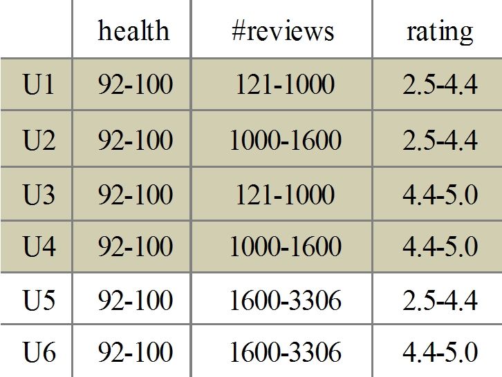
This article has been accepted for publication in a future issue of this journal, but has not been fully edited. Content may change prior to final publication. Citation information: DOI
                                               10.1109/TKDE.2014.2365792, IEEE Transactions on Knowledge and Data Engineering
                                                                                                                                                                     4

          is very difficult to decide the best way to create the                             It should be noted that although the location-aware
          ranges. What is more, the query processing is not                               objects can be well stored in a relational database,
          straightforward. Just consider the predicate health ≥                           the current support for LKQ, not to mention the
          75. As the predicate cannot be perfectly transformed                            GLRQs, in RDBMS is very poor. In fact, we have
          into a set of keywords, some post processing stages                             loaded our experimental data into MySQL and a
          are necessary, such as result verification.                                     commercial RDBMS, built all the necessary indexes
                                                                                          (spatial indexes on the locations, full-text indexes on
          LKQ-first method (LKQ-F). This method first com-
                                                                                          the texts, and B+ -tree indexes on other attributes),
          putes the results of the query without predicate (an
                                                                                          and then posted several LKQs and GLRQs in SQL
          LKQ query), and then validates the results obtained
                                                                                          language on the databases. The observed query plans
          against the query predicate.
                                                                                          show that both RDBMSs process the LKQs in a rather
             If the ranking function consists of only spatial prox-
                                                                                          naive way (direct sorting), and the GLRQs in the
          imity and textual relevance, the efficiency of LKQ-F
                                                                                          predicate-first way. Therefore, the built-in capabilities
          depends on the selectivity of the query predicate. Let
                                                                                          of RDBMS are far from satisfactory.
          sel(Q.P ) be the selectivity of the query predicate Q.P ,
                                                                                             According to the semantics of GLRQs, objects are
          where the selectivity is defined as the proportion of
                                                                                          not returned as final results if they do not satisfy
          objects matching the predicates in all the objects. Then
                                                                                          the query predicate, or they have low scores. There-
          given an object O, the possibility of O satisfying Q.P
                                                                                          fore, we can prune the results using two strategies:
          is sel(Q.P ). Let x be the number of additional results
                                                                                          predicate-based pruning and score-based pruning,
          needed to obtain the final top-k results. The value
                                                                                          which prune the results based on the satisfiability and
          of x follows the negative binomial distribution with the
                                                                                          scores, respectively. The LKQ-F and PF solutions are
          probability density function as follows
                                                                                          not efficient because they conduct the predicate-based
                                                                                          pruning and score-based pruning in separate stages,

                                  x+k−1
                     Pk,p (x) =              · pk · (1 − p)x                              leading to large numbers of intermediate results. To
                                   k−1
                                                                                          achieve good query performance, it is essential to
          where p = sel(Q.P ). For example, suppose p = 0.01                              prune the objects that are not in the top-k results
          and k = 3, then the probability of obtaining 3 results                          as early as possible. In this work, we propose a
          satisfying the query predicate after generating even                            framework to index and process the GLRQ, which
          100 results is still 0.0794.                                                    combines predicate-based pruning and score-based
            If attributes other than the location and text are                            pruning in a systematic manner.
          involved in the ranking function, the efficiency of                                Without loss of generality, we assume that the
          LKQ-F is even worse. That is because LKQ-F does not                             spatial locations have been indexed by an R-tree, and
          take the attribute scores into account when generating                          other attributes have been indexed by B+ -trees.
          the intermediate LKQ results. Consequently, more in-
          termediate results are generated, until it is guaranteed                        4     T HE LINQ F RAMEWORK
          that no better results can be found.
                                                                                          In this section, we present the LINQ framework to
            If the query does not contain keyword constraints,
                                                                                          support the indexing of location-aware objects and
          LKQ-F does not apply at all.
                                                                                          query processing of GLRQs. In the framework, there
            Therefore, the LKQ-F method is not a suitable so-
                                                                                          is a synopses tree summarizing numeric attributes,
          lution.
                                                                                          and a spatio-textual index built on locations and
          Predicate-first method (PF). In this approach, the                              keywords. We first introduce the index structure, and
          query predicate is evaluated to get a set of candi-                             then the query processing.
          dates, which are then scored according to the ranking
          function, and finally the k objects with greatest scores                        4.1     Synopses Tree
          are returned. As discussed in Section 1, this method
                                                                                          It is very common for a DBMS to build synopses
          generally has a very high cost.
                                                                                          on top of one or multiple attributes. The synopses
          R-tree based method (RT). Another approach is to                                are primarily used to estimate the selectivities of
          index the location and other attributes in one index,                           queries so that better query plans can be found. In
          such as R-tree. For the query Q4 in Example 3, if rating                        this work, we also make use of synopses, and the
          and health are also indexed together with the loca-                             motivation is similar: we use the synopses to estimate
          tions, the query can be processed easily. This approach                         the satisfiability of the query predicate. As the results
          has several shortcomings. First, as the R-tree has to                           cannot be obtained in one shot, we build a synopses
          index all the attributes, objects are nearly duplicated                         tree, instead of a synopsis, to guide the search.
          in the R-tree, and the redundancy would be very high.                              Basically, the synopses tree is a tree of synopses,
          Second, the R-tree must have a high dimensionality.                             where each node represents a synopsis of a dataset.
          Due to the curse of dimensionality [8], the method                              In the synopses tree, each leaf has a number of
          can hardly provide satisfactory performance.                                    pointers to objects. Each internal node has a number

                                 1041-4347 (c) 2013 IEEE. Personal use is permitted, but republication/redistribution requires IEEE permission. See
                                         http://www.ieee.org/publications_standards/publications/rights/index.html for more information.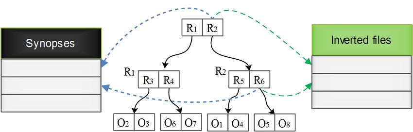
This article has been accepted for publication in a future issue of this journal, but has not been fully edited. Content may change prior to final publication. Citation information: DOI
                                               10.1109/TKDE.2014.2365792, IEEE Transactions on Knowledge and Data Engineering
                                                                                                                                                                     5

          of entries, where each entry consists of a synopsis                             explanation of the modeling method is presented in
          and a pointer to a child node. Each node or entry                               Appendix A.
          encloses a set of objects. We can imagine that there is                            Example 4: Take the data in Fig. 2 as an exam-
          a dataset associated with each node or entry, which                             ple. The method first builds a model called moral
          contains all objects enclosed. Let N (e) be a node                              graph (e.g. Fig. 3(a)), where each node represents
          (an entry) in the synopses tree. We use N.D (e.D)                               an attribute, and each edge represents a dependency
          to denote the imaginary dataset corresponding to N                              between a pair of attributes. Then, a junction tree is
          (e), and N.syn (e.syn) the synopsis of N.D (e.D). In                            created based on the moral graph, where an attribute
          a synopses tree, if a node N1 is a child of N , then                            is put together with the attribute it depends on. The
          N1 .D ⊆ N.D; if N1 , · · · , Nn are the children of N ,                         junction tree is shown in Fig. 3(b). According to
          then N.D = N1 .D ∪ · · · ∪ Nn .D. Given a dataset D, let                        the junction tree, we keep distributions of {#reviews,
          ST be the synopses tree built over D, then the root of                          health} and {#reviews, rating}. Other distributions
          ST summarizes the whole dataset D, and each node                                can be derived from the two distributions. In other
          summarizes a subset of D. What is more, the nodes                               words, we keep two 2D histograms instead of a 3D
          near the root provide summaries of larger subsets of                            histogram.
          the dataset.
             The strength of synopses tree is that, as each en-                           4.2.2 Global buckets
          try in a non-leaf node contains a synopsis, we can                              The work of [10] addresses the problem of how to
          estimate the satisfiability of a query predicate when                           construct a single nD histogram over a dataset. In
          visiting the entry, making it possible to do predicate-                         our work, we need to build a tree of synopses. If the
          based pruning. We will show in detail how to process                            nD-histograms in the synopses tree are constructed
          GLRQs later on.                                                                 independently, the cost would be too high. In the
                                                                                          following sections, we propose a method to construct
          4.2    Design of Synopses Tree                                                  the synopses with reduced cost.
                                                                                             We notice that, the synopses in the synopses tree
          In the following, we give more details about the                                are not independent. First, the datasets of different
          synopses tree.                                                                  nodes may be similar or overlapping. Second, the
                                                                                          dataset of a node at a higher level is a superset of
          4.2.1 Factorized multi-dimensional histogram                                    that of its descendants. Considering the characteristics
          There are different families of synopses, such as ran-                          above, we construct the histograms in a holistic way.
          dom samples, histograms, wavelets and sketches [9].                             Specifically, we construct a set H = {H1 , H2 , · · · } of
          We use histograms in this work, as histograms have                              global histograms for the whole dataset D, where
          been extensively studied and have been incorporated                             Hi = {Bi1 , Bi2 , · · · } is a global histogram, and Bij is a
          into virtually all RDBMSs.                                                      bucket the histogram Hi . The set of global histograms
             As more than one attributes are concerned, we                                is used by all entries in the synopses tree. Let  S B be the
          build multi-dimensional histograms to summarize the                             set of buckets in all histograms, i.e. B = i Hi , and
          datasets. Multi-dimensional (nD) histogram has been                             |B| be the number of buckets in B. For any entry e, an
          widely used to summarize multi-dimensional data.                                array e.b with |B| elements is maintained, where each
          Basically, an nD histogram is obtained by partitioning                          element in the array is the statistics about the e.D in a
          the multi-dimensional domain into a set of hyper-                               bucket. Thus the array records the summary statistics
          rectangular buckets, and then storing summary infor-                            of e.D.
          mation for each bucket. As a synopsis, nD histogram                                Example 5: Consider the Example 4. We construct
          is able to provide accurate approximation, but it is                            histograms for the 2D datasets (#reviews, health) and
          very expensive to construct and maintain an nD his-                             (#reviews, rating). The global histograms are shown
          togram. To reduce the complexity of nD histogram, we                            in Fig. 4(a) and (b). Here we assume 8 buckets are
          use the graphical model of Tzoumas et al [10] to factor                         available, and the equi-depth bucketing scheme is
          the nD data distribution into two-dimensional (2D)                              adopted. The right part of Fig. 4 shows the local
          distributions. The effectiveness of this method has                             information kept by each entry, where R1 , · · · , R6 are
          been verified. By this way, we can provide accurate                             the entries in the R-tree (the R-tree is presented in
          approximations of the joint data distributions with                             Fig. 5). In this example, we just keep the count of
          low cost.                                                                       objects falling in each bucket (more discussions will
             The graphical modeling of a dataset generates a                              be presented later).
          model called junction tree. In our setting, the junction                           By using global histogram definitions, i.e. global
          tree is a tree structure where each node is a pair                              buckets, the construction cost and storage overhead of
          of attributes. Then, according to the junction tree,                            histograms are decreased. This is because the global
          the joint distribution of multiple attributes can be                            histograms are constructed and stored only once.
          factorized into a set of 2D distributions. An example                           For each entry in a non-leaf node, only some local
          of junction tree is shown below. A more detailed                                statistics are kept.

                                 1041-4347 (c) 2013 IEEE. Personal use is permitted, but republication/redistribution requires IEEE permission. See
                                         http://www.ieee.org/publications_standards/publications/rights/index.html for more information.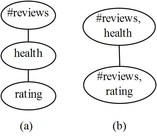
This article has been accepted for publication in a future issue of this journal, but has not been fully edited. Content may change prior to final publication. Citation information: DOI
                                               10.1109/TKDE.2014.2365792, IEEE Transactions on Knowledge and Data Engineering
                                                                                                                                                                     6

          Fig. 3. An example of junction tree. (a)                  Fig. 4. The histograms constructed for the example dataset. (a) H1,
          The moral graph, (b) The junction tree                    (b) H2, (c) local information

          4.2.3     Compact local information                                             #reviews ≤ 179, 83 ≤ health ≤ 91} in Fig. 4. According
                                                                                          to the splitting method, the #reviews dimension will
          A bucket in the global histograms stands for a hyper-
                                                                                          be split three times into 8 ranges. and dimension
          rectangle within the domain of data. To approximate
                                                                                          health will be split twice. We can define a default
          the data points falling in the hyper-rectangle, some
                                                                                          order on the partitions, e.g., (#reviews=[121, 127],
          statistics about the distribution of data in the rectangle
                                                                                          health=[83, 84]), (#reviews=[121, 127], health=[85, 86]),
          are needed. In Example 5, for each entry, we keep
                                                                                          · · · . If the first two bits of a bit string is “10”, it
          the count information regarding each bucket. In fact,
                                                                                          indicates that there are points in the first partition
          as we are only concerned with the satisfiability of
                                                                                          while not in the second partition.
          query predicate in this work, some simple statistics
          is enough.
                                                                                          4.2.4     Summary of the synopses tree
             For example, consider the 2D bucket B11 in Fig. 4,
          it corresponds to a rectangle {121 ≤ # reviews ≤                                The key points in the design of synopses tree is
          179, 83 ≤ health ≤ 91}. Suppose we are interested in                            summarized as follows.
          objects satisfying P1 : health ≥ 85. If we know that the                           • Conceptually, each synopsis is composed of two
          bucket B11 is not empty, then we can estimate that the                                parts: the synopsis definition, and the statistics
          predicate P1 holds on the bucket. From this example,                                  about data. Actually, the synopsis definition is the
          we can see that it is possible to do estimation with                                  same for all entries, so there is only one copy of
          only one bit kept for a bucket, indicating whether the                                global synopsis definition.
          bucket is empty or not. However, the estimation error                              • Each synopsis is an nD histogram, which is de-
          would be high if the bucket covers wide ranges. To                                    composed into multiple 2D histograms. In the
          improve the accuracy of estimation, more in-bucket                                    global, the boundaries of the buckets, and the
          information is needed.                                                                split information are maintained.
             In this work, we use a compact bit-based represen-                              • The local description of an entry is a set of
          tation of the local information in each bucket. We split                              simple M -bit strings, each corresponding to a
          each bucket into M partitions, and then stores a M -                                  bucket in a 2D histogram. The data distribution
          bit string where each bit is 1 if the corresponding                                   of each bucket is interpreted on the basis of global
          partition is not empty or 0 otherwise. According to                                   histogram when necessary.
          the practice of [11], 32 and 64 are good choices for                               Example 7: The synopses tree of the dataset in Fig. 2
          M on 32-bit and 64-bit platforms, respectively. By                              is illustrated in Fig. 5. As discussed earlier, two 2D
          this method, the accuracy of synopsis is improved                               histograms H1 and H2 are constructed, each with 4
          by an order of M . In our implementation, we choose                             buckets. For each entry in a non-leaf node, a syn-
          M = 32.                                                                         opsis is maintained, which keeps information about
             The M partitions are obtained by successive binary                           the buckets in the global histogram. For example, to
          splits of dimensions in a round-robin manner. For                               describe the data distribution of an entry R6 with
          example, if the buckets have 3 dimensions x1 , x2 , x3 ,                        respect to B11 , a 32-bit string is used (M = 32).
          and M = 32, then one split order is x1 , x2 , x3 , x1 , x2 .                    Therefore, the synopsis of an entry is an array of
          Each split is done on the middle, so that the partitions                        bit strings corresponding to the buckets in the global
          are equally sized. To interpret the 32-bit array when                           histograms.
          estimate, the boundaries of the partitions should be                               We estimate the space consumption of the synopses.
          known. For this purpose, we keep the splitting in-                              Maintaining the boundaries of a bucket needs at
          formation, and the correspondence between the bits                              most 4 numeric values, i.e. 32 bytes. Thus the global
          and the partitions. As all the buckets are split in the                         histogram requires 32 · |B| bytes. For each entry in the
          same way, this information can be stored only once                              non-leaf node, 32 · |B| bits or 4 · |B| bytes are needed
          as background information.                                                      (assume M = 32). The total space of the synopses is
             Example 6: Still consider the 2D bucket B11 : {121 ≤                         32 · |B| + 4 · |N | · |B| bytes, where |N | is the number of

                                 1041-4347 (c) 2013 IEEE. Personal use is permitted, but republication/redistribution requires IEEE permission. See
                                         http://www.ieee.org/publications_standards/publications/rights/index.html for more information.
This article has been accepted for publication in a future issue of this journal, but has not been fully edited. Content may change prior to final publication. Citation information: DOI
                                               10.1109/TKDE.2014.2365792, IEEE Transactions on Knowledge and Data Engineering
                                                                                                                                                                     7

          Fig. 5. An example of synopses tree                                             Fig. 6. The structure of the combined index

          non-leaf entries in the tree. Obviously, the overall cost                          S2I maps each distinct term to an aggregated R-tree
          is dominated by the second part. To reduce the space                            (aR-tree) [13] or block file, depending on whether the
          cost, we can reduce the number of buckets (|B|) in the                          term is a frequent term or not. It is possible to merge
          global histograms. Note that each bucket is divided to                          the aR-tree with synopses tree. However, that will
          32 partitions, so with |B| buckets, we obtain 32 · |B|                          significantly increase the size of the index, making it
          partitions. The accuracy of the synopsis is propor-                             unaffordable. It is very difficult, if not impossible, to
          tional to the number of partitions, therefore, we can                           combine the synopses tree with the block file, because
          choose a moderate number of buckets in the global                               the synopses tree is a hierarchical data structure, while
          histograms. For example, from 32 buckets we can                                 the block file is a plain flat file. In the following, we
          get 1024 partitions, a practical number for estimation.                         integrate the synopses tree with IR-tree to process the
          Another optimization is that the synopsis of an entry                           GLRQ.
          is represented in bit strings, which can be compressed
          to save space. In fact, the synopsis of an entry far
          from the root will have very sparse bit string (many                            4.4     Query Processing
          “0”s), thus can achieve a high compression rate. In                             In this section, we discuss the query processing algo-
          our implementation, the bit strings are compressed                              rithms for the GLKQs.
          using EWAH technique [12], which demonstrates a
          high compression rate. Note that the compression will
          not introduce any noises. Using these methods, we are                           4.4.1     Algorithm framework
          able to reduce the space consumption to a low level.                            The algorithm framework (Algorithm 1) exploits the
                                                                                          well-known best-first strategy [14] to search the com-
          4.3    Combining Synopses Tree with Other Indexes                               bined index. In the algorithm, a priority queue Queue
                                                                                          is used to keep track of the nodes and objects to
          The synopses tree summarizes the distribution of
                                                                                          explore in decreasing order of their scores. maxf (e, Q)
          numeric attributes. It is able to address part of the
                                                                                          is the maximum matching score of entry e to query
          GLRQ processing problem. For example, for the query
                                                                                          Q, which are used as the keys of entries in the queue.
          in Example 3, the synopses tree can be used to find
                                                                                          The computation of maxf (·, ·) will be explained later.
          the objects that satisfy rating ≥ 4.0 ∧ health ≥ 95, and
                                                                                          T opK keeps the current top-k results. The R-tree is
          have greatest partial scores according to the function
                                                                                          traversed in a top-down manner. At each node N ,
          0.05 × O.rating
                     5.0  + 0.05 × O.health
                                       100  . To answer the GLRQ,
                                                                                          if N is an internal node instead of a leaf (line 10),
          we need to combine synopses tree with other indexes
                                                                                          for each entry e in node N , the algorithm estimates
          on locations and texts.
                                                                                          maxf (e, Q). If maxf (e, Q) > 0, it implies that there
             The state-of-the-art index structures supporting lo-
                                                                                          may be objects enclosed by e satisfying the query
          cations and texts are the IR-tree family [2], [3] and
                                                                                          predicate, so e with maxf (e, Q) is added to the queue.
          S2I family [5]. The basic structure of IR-tree index
                                                                                          If N is a leaf, it computes the score of each entry
          is an R-tree, where each entry is associated with
                                                                                          (object) (line 19), and pushes the entries with non-zero
          an inverted file. Our synopses tree can be easily
                                                                                          scores to the queue. If N is an object, N is directly
          combined with IR-tree index. Fig. 6 illustrates the
                                                                                          reported as a top-k result. The algorithm terminates
          combined index structure, for the dataset shown in
                                                                                          if the top-k results have been found.
          Fig. 2. In the middle of the figure there is an R-tree
          indexing the locations of the objects. Each entry in the
          R-tree is associated with two additional components:                            4.4.2     Computing maximum scores
          the inverted file from the IR-tree, and the synopsis                            Given a query Q and a node N in the R-tree, we
          from the synopses tree. The inverted files and the                              compute a metric maxf (N, Q), which offers an upper
          synopses are stored separately from the R-tree. This                            bound on the actual scores of the objects enclosed by
          structure is flexible in that the structure of the R-tree                       N with respect to Q. That is,
          is not influenced by other parts, and the R-tree can be
          queried alone, with or without the inverted files and                              maxf (N, Q) = max{f (O, Q)|O is enclosed by N }
          the synopses.                                                                                                                     (2)

                                 1041-4347 (c) 2013 IEEE. Personal use is permitted, but republication/redistribution requires IEEE permission. See
                                         http://www.ieee.org/publications_standards/publications/rights/index.html for more information.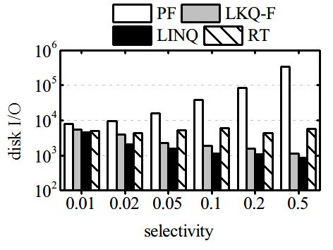
This article has been accepted for publication in a future issue of this journal, but has not been fully edited. Content may change prior to final publication. Citation information: DOI
10.1109/TKDE.2014.2365792, IEEE Transactions on Knowledge and Data Engineering
8
Algorithm 1 Search(index R, GLRQ Q) estimating for these nodes independently may take
1: T opK ← ∅ a long time. Considering the characteristics of the
2: Queue.push(R.root, 0) index structure, we devise a more efficient estimation
3: while Queue 6= ∅ do method.
4: (N, d) ← Queue.pop() Conceptually, we can think of the synopsis asso-
5: if N is an object then ciated with a node N as a multi-dimensional space
6: T opK.insert(N ) (called data space of N , denoted as ds(N )) consist-
7: if |T opK| = k then ing of hyper-rectangles. Similarly, a query Q can be
8: break considered as a set of hyper-rectangles (called query
9: end if space of Q, denoted as qs(Q)) encompassing the points
10: else if N is not a leaf node then satisfying the query predicate. Given a node N and
11: for entry e in N do a query Q, if ds(N ) intersects with qs(Q), then Q is
12: d ← maxf (e, Q) assumed to be satisfied at N , and we call ds(N )∩qs(Q)
13: if d > 0 then the relevant data space (RDS) of N with respect to Q,
14: Queue.push(e, d) denoted as rdsQ (N ) (we simply use rds(N ) when the
15: end if context is clear).
16: end for Our algorithm is described in Algorithm 2. It has
17: else two parts. In the first part, the RDS of the root root
18: for entry e in N do of the synopses tree is precomputed. The algorithm
19: d ← f (e, Q) traverses the junction tree in a leaf-to-root manner,
20: if d > 0 then and constructs the rds(root) incrementally. Note that
21: Queue.push(e, d) each node in the junction tree represents a clique,
22: end if containing a pair of attributes. For each clique C,
23: end for a partial RDS rdsC (root) is computed (line 5). Here
24: end if “partial” refers to the fact that only two attributes
25: end while are concerned here. Then it merges the partial RDS
26: return T opK with rds(root) (line 6), which will add at least one
dimension to rds(root). Initially, rds(root) is empty,
so the merging operation just assigns rdsC (root) to
According to formula 1, the formula can be rewritten rds(root). If rds(root) is not empty, the merging will
as follows. add a new dimension to rds(root). This is because
one attribute in C should have been seen in previous
maxf (N, Q)
cliques, only the unseen attribute will be added into
rds(root). After that, the dimensions that will not be
0 Q(N ) = ∅
used are removed to reduce the dimensionality of
= O∈Q(Nmax (g(prox(O, Q), rel(O, Q), rds(root).
)
s1 (O.A1 ), · · · )) otherwise The second part is invoked when visiting an entry.
(3) Given an entry e, it first dynamically computes rds(e).
where Q(N ) denotes the set of objects enclosed by N Let par(e) be the parent of e. It can be inferred
that satisfy the query predicate. that, rds(e) can be obtained by intersecting ds(e)
Therefore, to estimate maxf (N, Q), we need first with rds(par(e)). Therefore, rds(par(e)) can be reused
estimate whether Q(N ) is empty or not. Estimating and estimation at e can be accelerated. Line 2 to 8
Q(N ) is in fact estimating the satisfiability of a query, computes rds(e) according to the discussion above.
which is a special case of selectivity estimation. When Then, based on rds(e), the satisfiability of the query
Q(N ) is not empty, the value of maxf (N, Q) can be is estimated. If rds(e) is empty, it implies that the
estimated using the following formula: query predicate cannot be satisfied by the objects
enclosed by e. Otherwise, the algorithm estimates
maxf (N, Q) = g(prox(N, Q), rel(N, Q), s1 (N.A1 ), · · · ) maxf (e, Q) based on the stored keyword information
(4) and synopses according to formula 4.
where prox(N, Q) is the proximity between N.rect We use a concrete example to illustrate the process.
and Q.λ, rel(N, Q) is the text similarity between N.D Example 8: Recall the dataset in Fig. 2. The example
and Q.W , and si (N.Ai ) is the score computed from 2D histograms H1 and H2 have been presented in
the values of Ai in the dataset N.D. Example 5. As the dataset is tiny, we assume that
the buckets are not split any more. So each entry
4.4.3 Estimation in the R-tree (see Fig. 6) just keeps 8 bits indicating
Given a node N in R-tree, estimating Q(N ) is not whether there are descendant objects falling in the
difficult using the synopsis kept for N . However, buckets. Consider the query in Example 3. Recall that
as the algorithm needs to visit a number of nodes, the query predicate is “rating ≥ 4.0 ∧ health ≥ 95”.
1041-4347 (c) 2013 IEEE. Personal use is permitted, but republication/redistribution requires IEEE permission. See
http://www.ieee.org/publications_standards/publications/rights/index.html for more information.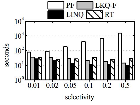
This article has been accepted for publication in a future issue of this journal, but has not been fully edited. Content may change prior to final publication. Citation information: DOI
                                               10.1109/TKDE.2014.2365792, IEEE Transactions on Knowledge and Data Engineering
                                                                                                                                                                     9

          Algorithm 2 Estimation
          Precompute(Junction tree J, global histograms H,
          query Q)
           1: let root be the root of the synopses tree.
           2: rds(root) ← ∅
           3: for clique C in J do
           4:                   . traverse J in a bottom-up way
           5:     compute the rdsC (root)
           6:     rds(root) = merge(rdsC (root), rds(root))
           7:     reduce rds(root) by removing the useless di-                            Fig. 7. An example of data space
              mensions
           8: end for
          Estimate maxf (e, Q)                                                            simpler. For example, for LKQs, the query processing
           1: Let par(e) be the parent of e                                               algorithm behaves the same as IR-tree. If no key-
           2: rds(e) ← rds(par(e))                                                        words are involved in the query, inverted files are not
           3: for clique C in J do                                                        needed. These algorithms are not presented to save
           4:     rds(e) = rds(e) ∩ dsC (e)                                               space.
           5:     if rds(e) = ∅ then
           6:         break                                                               4.5     Maintenance of Indexes
           7:     end if                                                                  The indexes in LINQ can be implemented within or
           8: end for                                                                     outside a database. The core data structures we need
           9: if rds(e) = ∅ then                                                          are just R-trees and B+ -trees, which are available in
          10:     maxf (e, Q) ← 0                                                         mainstream databases. The maintenance of the IR-
          11: else                                                                        tree has been discussed in [3]. Therefore, we focus
          12:     compute maxf (e, Q)                                                     on the synopses tree here. We assume the domains of
          13:                     . compute based on formula 4                            numeric attributes do not change and are known in
          14: end if                                                                      advance.
          15: return maxf (e, Q)
                                                                                          Construct. In LINQ, the synopses are stored sepa-
                                                                                          rately from the R-tree, therefore, the R-tree can be
                                                                                          constructed as usual. Then, the global histograms
          The junction tree has been constructed in Fig. 3. Let                           are built, followed by the synopses (bit strings)
          C1 and C2 refer to the cliques of {#reviews,health}                             of the nodes. The bit strings have the salient fea-
          and {#reviews,rating}, respectively. In the precom-                             ture that, N.syn can be obtained by superimposing
          putation step, rds(root) is computed. We can see                                N1 .syn, · · · , Ni .syn, where N1 , · · · , Ni are the children
          from Fig. 7 that rds(root) contains 6 hyper-rectangles                          of N . This feature can be used to speedup the con-
          U1 , · · · , U6 . Note that the space is actually a plane                       struction of synopses, since only bit strings of leaf
          (92 ≤ health ≤ 100). Consider the entry R1 . According                          nodes need to be constructed from the scratch.
          to the information in Fig. 4, we can get its data space
          ds(R1 ) from the non-empty buckets in H1 and H2 . As                            Insert. Insertion to the synopses tree is described in
          U5 and U6 intersect with ds(R1 ), rds(R1 ) is {U5 , U6 }.                       Algorithm 3, which is adapted from the standard
          Now consider the entry R4 . As rds(R1 ) does not                                algorithm in R-tree [15]. At line 3, the synopsis of N is
          intersect with dsC1 (R4 ), rds(R4 ) is empty, thus R4 can                       updated, i.e. some bits are changed from 0s to 1s. The
          be pruned.                                                                      update is trivial as the new data O.D only influences
             Note that Algorithm 2 as well as Example 8 just il-                          several partitions. When the leaf N is split into two
          lustrates the main ideas. In implementation, we do not                          ones N1 and N2 (line 6), the N1 .syn and N2 .syn are
          actually construct and maintain the hyper-rectangles.                           just computed from their entries. The update at line 10
             An important feature of the metric maxf (N, Q) is                            and line 13 are similar. As the updates are propagated
          that it inherits the nice features of the R-tree for query                      in a bottom-up way, the synopses of nodes at a
          processing [14].                                                                higher level can be obtained by just superimposing
                                                                                          the synopses of their children.
             Theorem 1: Given a query Q and a node N where
          N encloses a set O0 of objects, we have ∀O ∈                                    Delete. When some objects are deleted, the synopses
          O0 (maxf (N, Q) ≥ f (O, Q)).                                                    of affected leafs have to be recomputed. If the deletion
             Theorem 1 guarantees that the metric maxf (N, Q)                             leads to reinsertion or merge of nodes, the affected
          can be safely used to direct the traversal of the index                         internal nodes have to be updated. Again, update of
          tree. Due to space constraint, the proof of Theorem 1                           internal nodes is done by superimposing the synopses
          is presented in Appendix B.                                                     of their children. Due to space limitation, the algo-
             For some subsets of GLRQs, the algorithms can be                             rithm is not presented.

                                 1041-4347 (c) 2013 IEEE. Personal use is permitted, but republication/redistribution requires IEEE permission. See
                                         http://www.ieee.org/publications_standards/publications/rights/index.html for more information.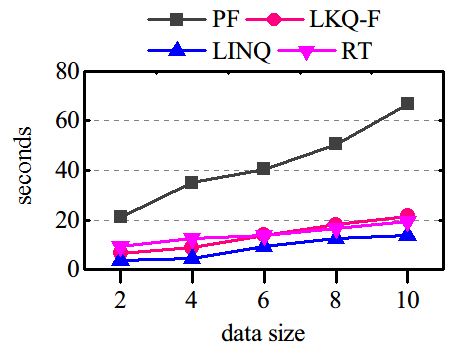
This article has been accepted for publication in a future issue of this journal, but has not been fully edited. Content may change prior to final publication. Citation information: DOI
                                               10.1109/TKDE.2014.2365792, IEEE Transactions on Knowledge and Data Engineering
                                                                                                                                                                    10

          Algorithm 3 Insert(O)                                                           picked from a Twitter dataset crawled by us. The
           1: N ← chooseLeaf(O.λ)                                                         average number of words per object is 7.4. The values
           2: Add O.λ to N                                                                of each attribute are randomly and independently
           3: Update N.syn                                                                generated, following a normal distribution. The do-
           4: if N needs to be split then                                                 mains and cardinalities of the attributes are different.
           5:     {N1 , N2 } ← N .split()
                                                                                          Setup. All algorithms were implemented in C++.
           6:     Compute N1 .syn and N2 .syn
                                                                                          The objects are stored in a B+ -tree file. We use the
           7:     if N is root then
                                                                                          same settings as in IR-tree [2]. All experiments are
           8:         Initialize a new node N0 , let N1 and N2 be
                                                                                          conducted on a machine with i7 3.4G CPU, 4G main
              children of N0 , and set N0 be the new root
                                                                                          memory and 500G hard disk, running Windows 7. All
           9:     else
                                                                                          indexes are disk-resident. When constructing the his-
          10:         Ascend from N to the root, adjusting the
                                                                                          tograms, the bucketing scheme is maxdiff [17], which
              covering MBRs, updating synopses and propagat-
                                                                                          has shown good accuracy [9]. A B+ -tree is built on
              ing node splits as necessary
                                                                                          each numeric attribute, so that PF can utilize the
          11:     end if
                                                                                          indexes to accelerate the predicate-based filtering. The
          12: else if N is not root then
                                                                                          metrics considered are processing time and I/O cost,
          13:     Update the covering MBRs and synopses of the
                                                                                          where the latter is measured by the number of disk
              ancestors of N
                                                                                          page accesses.
          14: end if
                                                                                             The experimental settings are shown in Table 2.
                                                                                          Some parameters have more than one value, which
                                                                                          is used when studying the impacts of the parameters.
          5     E XPERIMENTAL               STUDY
                                                                                          The default values are used unless otherwise speci-
          In this section, we evaluate the performance of the                             fied.
          proposed method.                                                                   The ranking function in a GLRQ combines the
                                                                                          spatio-textual similarity and scores of other attributes.
          5.1    Experimental Setting                                                     We employ a linear combining function as in previous
                                                                                          works [2], [5], like the one in Example 3. The weights
          Algorithms. The following methods are evaluated                                 of different parts may influence the performance.
          in the experiments: LKQ-naive, LKQ-F, PF, RT and                                Since there are many weights in the ranking function,
          LINQ, where the former four methods have been in-                               it is not easy to figure out the impact of a certain
          troduced in Section 3, and LINQ denotes our method.                             weight. Therefore, we simplify the ranking function
          To make RT also support keyword search, each node                               as follows.
          in the R-tree is also associated with an inverted file as
          in IR-tree [2].                                                                   f (O, Q) = α×st-sim(O, Q)+(1−α)×att-score(O) (5)

          Data. We use both real and synthetic data for the                               where st-sim(O, Q) and att-score(O) are the spatio-
          experiments.                                                                    textual similarity and score derived from attribute val-
             The real dataset is the Amazon product reviews                               ues, respectively; they themselves are combinations of
          dataset [16], which consists of product reviews ob-                             several factors. Then, we investigate the performance
          tained from www.amazon.com. In our experiments,                                 when the parameter α changes. For st-sim(O, Q), we
          we use the data describing members and their re-                                do not dig into the performance issues when the
          views. After cleaning, the dataset has about 5.8M                               spatial proximity or text relevance has varying impor-
          objects and 5 attributes in addition to the geo-location                        tance. That has been the topic of previous works [18].
          and text attribute. Each object in the dataset represents                       We just treat different factors equally important. The
          a review, described by rating, number of feedback,                              att-score(O) is treated similarly. To give an example,
          number of helpful feedback, review body, consumer’s                             if the α parameter in Formula 5 is 0.6, then the actual
          location, rank, number of reviews, and so on. The                               function would be like this:
          review body is a piece of text whose length (number                              f (O, Q) =0.6 × (0.5 × prox(O, Q) + 0.5 × rel(O, Q))+
          of keywords) ranges from 10 to 3345. We can think of
                                                                                                                  O.rating          O.health
          an application where one tries to find some consumers                                      0.4 × (0.5 ×          + 0.5 ×           )
          according to their locations, reviews, and other infor-                                                    5.0              100
          mation, thus the GLRQ can be adopted.
             In the synthetic dataset, each object is composed                            5.2     Performance on Real Dataset
          of 9 attributes, including the coordinates, the text
                                                                                          In this section, we report the experimental results on
          description, and 6 numeric attributes. The size of the
                                                                                          real dataset.
          synthetic dataset varies in the experiments, and will
          be pointed out later. The coordinates are randomly                              Index construction cost. We first evaluate the con-
          generated in (0, 100), and the texts are randomly                               struction costs of various methods. The cost of an in-

                                 1041-4347 (c) 2013 IEEE. Personal use is permitted, but republication/redistribution requires IEEE permission. See
                                         http://www.ieee.org/publications_standards/publications/rights/index.html for more information.
This article has been accepted for publication in a future issue of this journal, but has not been fully edited. Content may change prior to final publication. Citation information: DOI
10.1109/TKDE.2014.2365792, IEEE Transactions on Knowledge and Data Engineering
11
TABLE 2 We can see from Fig. 9 that, when the selectivity
Experimental settings increases from 0.01 to 0.5, the processing time and disk
Parameter Values
I/O of PF increase, because PF is very sensitive to the
Page size 4KB predicate selectivity. The performance of RT fluctuates
R-tree fanout 100 when the selectivity of query predicate changes, but
Selectivity 0.01, 0.02, 0.05, 0.1, 0.2, 0.5 there is no clear trend. For LKQ-F and LINQ, we
Number of predicates 1, 2, 3, 4, 5
Number of results 1, 5, 10, 20, 35, 50 can see that as the selectivity increases (i.e. the query
Number of buckets 512, 768, 1024, 1536, 2048 predicate is less selective), the elapsed time and disk
Buffer capacity (%) 1, 2, 5, 10, 20, 50 I/O cost go down. The reasons are different. For LKQ-
α 0.1, 0.3, 0.5, 0.7, 0.9
F, that is because when the predicates are not selective,
(The default values are presented in bold) the results of the LKQs have higher probabilities
of satisfying the predicates, thus less intermediate
results are produced. For LINQ, the performance can
dex is measured by its construction time and occupied be explained by false positives. False positives are
space. introduced if some nodes of the R-tree are estimated
The costs of various methods are shown in Fig. 8, to satisfy the predicate, but actually they do not.
where naive refers to the LKQ-naive method. Note that Obviously, false positives lead to unnecessary com-
we have to abort the indexing process of the naive putations. When the predicates are not selective, the
method, because it takes so much time and space. We number of false positives decreases, so unnecessary
can see that, naive and LKQ-F show greatest index computations are reduced.
costs. The high index cost of LKQ-based methods has Varying the number of predicates. We change the
also been observed in other works [18], which makes number of selection predicates in the queries from 1
them less attractive. PF has the lowest cost among to 5. For each number of predicate, we generate a set
the methods, because it requires only the availability of 50 queries. Each selection predicate is of the form
of B+ -trees. RT and LINQ have moderate costs. The v1 ≤ attr ≤ v2 . The predicates in each query involve
majority of their costs are due to the inverted files. different attributes. The results are shown in Fig. 10.
Compared with RT, LINQ has smaller index size, We can see that, when the number of predicates
but more indexing time. The time spent on building change, the time and I/O cost of LINQ have subtle
the synopses tree consists of two parts: the time of changes. This is because when more predicates are
building global histograms, and the time of building present in the query, more attributes are involved,
synopses of nodes, where the former accounts for and estimating the satisfiability and scores is a bit
the vast majority. Note that the high cost of building more complicated. The disk I/O does not change
histograms is not our fault, but a well-known problem much, because the synopsis of a node (the bit strings)
[9]. And, the global histograms are not designed solely is stored as a whole. The PF is very sensitive to
for our problem, it can be used by other components, the number of predicates, because more B+ -trees are
e.g. the query optimizer, of the system. In fact, if we searched when the number of predicates increases.
rip that part off, the additional cost of building the The performance of LKQ-F does not change much,
synopses of the nodes is very low. Still, the cost of because its query performance is independent of the
building synopses can be reduced by using a simple number of predicates.
bucketing strategy, such as equi-depth, and fewer
buckets. Varying K. We examine the performances of various
We also show the costs when the dataset has no methods when the number K of requested results
text attributes in Fig. 8(c) and (d). It can be clearly changes. We first generate 50 distinct queries. For each
seen that LINQ occupies the least space, but it has query, we vary K from 1 to 50. Then the results are
the greatest indexing time. The reason is similar. averaged for each number of K. As seen from the
In the following sections, we consider only four Fig. 11, the cost of PF keeps almost constant, because
methods: LKQ-F, PF, LINQ and RT. We rule LKQ- the number of candidates satisfying the query does
naive out because it is deemed impractical, due to its not change. Other methods have growing costs as
huge space and time requirement. K increases, but generally, the increase rate is not
high. LINQ is always better than LKQ-F in terms
Processing time and disk I/O. We generate 50 distinct of elapsed time and disk I/O, and the gap between
queries, involving different attributes. For each query, their performance is enlarged when K increases. The
we fix the location and the keywords, and vary the performance can be explained that, when K is larger,
selectivities of query predicates from 0.01 to 0.5 by LKQ-F needs to explore much more results, resulting
changing the predicates. By this way, we obtain six in more disk page accesses.
query sets, corresponding to the six different selectiv-
ity levels. The processing times and I/O costs of the Varying the number of buckets. We change the
queries are averaged for each set. number of buckets from 512 to 2048, and monitor 1)
1041-4347 (c) 2013 IEEE. Personal use is permitted, but republication/redistribution requires IEEE permission. See
http://www.ieee.org/publications_standards/publications/rights/index.html for more information.You can also read