Understanding the mesoscopic scaling patterns within cities
←
→
Page content transcription
If your browser does not render page correctly, please read the page content below
Understanding the mesoscopic scaling patterns within cities

                                                                          Lei Dong,1, 2 Zhou Huang,1 Jiang Zhang,3 and Yu Liu1, ∗
                                                                1
                                                                    Institute of Remote Sensing and Geographical Information Systems,
                                                                                    School of Earth and Space Sciences,
                                                                                  Peking University, Beijing 100871, China
                                                                    2
                                                                        Senseable City Lab, Department of Urban Studies and Planning,
arXiv:2001.00311v1 [physics.soc-ph] 2 Jan 2020

                                                                Massachusetts Institute of Technology, Cambridge, MA 02139, USA
                                                         3
                                                             School of System Science, Beijing Normal University, Beijing 100875, China

                                                                                                 Abstract
                                                     Understanding quantitative relationships between urban elements is crucial for a wide range of
                                                 applications. The observation at the macroscopic level demonstrates that the aggregated urban
                                                 quantities (e.g., gross domestic product) scale systematically with population size across cities, also
                                                 known as urban scaling laws. However, at the mesoscopic level, we lack an understanding of whether
                                                 the simple scaling relationship holds within cities, which is a fundamental question regarding the
                                                 spatial origin of scaling in cities. Here, by analyzing four large-scale datasets covering millions of
                                                 mobile phone users and urban facilities, we investigate the scaling phenomena within cities. We find
                                                 that the mesoscopic infrastructure volume and socioeconomic activity scale sub- and super-linearly
                                                 with the active population, respectively; however, for a same scaling phenomenon, the power-law
                                                 exponents vary in cities of similar population sizes. To explain these empirical observations, we
                                                 propose a conceptual framework by considering the heterogeneous distributions of population and
                                                 facilities, and the spatial interactions between them. Analytical and numerical results suggest that,
                                                 despite the large number of complexities that influence urban activities, the simple interaction rules
                                                 can effectively explain the observed regularity and heterogeneity in scaling behaviors within cities.

                                                 Keywords: urban scaling, mobile phone data, infrastructure, socioeconomic activity, spatial interactions

                                                 ∗
                                                     liuyu@urban.pku.edu.cn

                                                                                                    1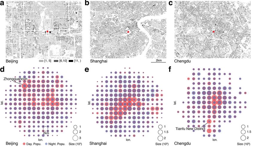
INTRODUCTION

   In spite of the complexity and variety of cities, it turns out that various macroscopic
properties related to urban activities Y , such as gross domestic product and road networks,
scale with the population size P in a surprisingly simple power-law manner: Y ∼ P β ,
where β is a scaling exponent (or an elasticity, in economic terms) that characterizes the
non-linear properties of urban systems [1]. In the past decades, the macroscopic urban
scaling phenomena have drawn great scientific interest in physics [2–5], economics [6, 7],
urban studies [8, 9], and many other fields [10–12]. And data in many urban systems
have demonstrated that these power-law relationships remain remarkably stable in different
countries [1, 5] and historical periods [13, 14].

   At the mesoscopic level, however, whether the relationships between urban characteristics
obey some universal patterns remains poorly understood. Here, the notion of the mesoscopic
level means a spatial scale around a few kilometers within cities, which is the most commonly
used spatial unit for urban research and urban planning [15]. Moreover, a striking variation
in population and socioeconomic density emerges at this spatial level [16–18]. Yet, current
urban scaling frameworks ‘ignore’ those heterogeneous distributions as they usually model
a city as a whole and study the macroscopic scaling phenomena across cities [3, 6, 12, 19–
21] or the temporal dynamics of individual cities [22–24]. (Ref. [25] compares the cross-
sectional and temporal scaling analyses at the macroscopic level.) Several key questions
at the mesoscopic level remain unanswered: do sub-units within a single city follow the
power-law scaling as observed for systems of cities? What is the mechanism behind the
‘potential’ scaling patterns within cities? Answering these questions is critical to reach a
better understanding of urban systems.

   Our limited understanding of intra-urban scaling phenomena stems from the lack of gran-
ular data documenting the spatial distributions of urban elements. Meanwhile, increasing
urban dynamics presents further challenges to the data and measurement issue [26]. For
instance, population – the key urban element – is quite dynamic within cities, making it
‘inaccurate’ when measuring population distribution by static data like census data. As the
census population only reflects a snapshot of the nighttime distribution of residents, the day-
time density of the urban center is highly underestimated (Fig. 1 and Supplementary Fig.
1). Recently, researchers have taken crucial steps in mapping the dynamic population [27]

                                              2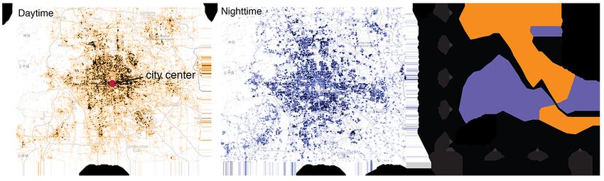
or considering three-dimensional building morphologies [28–30] in the within-city analysis.
Nevertheless, quantitative relations between urban elements are still far from clear.
   Here, benefiting from the revolution of big data, we analyze the quantitative relationships
between population, infrastructure, and socioeconomic activity at the mesoscopic level of ten
Chinese cities: Beijing, Chengdu, Hangzhou, Jinan, Nanjing, Shanghai, Shenzhen, Suzhou,
Xi’an, and Zhengzhou (Supplementary Table 1). These cities locate in different geographic
regions of China, which helps test the robustness of our findings. To derive the quantita-
tive relationship between urban elements, we use four extensive micro-datasets, including
a granular mobile phone dataset covering 107 million people, a building dataset containing
the three-dimensional information of ∼ 2 million buildings, a firm dataset recording ∼ 13
million firms, and a point of interests (POIs) dataset with approximately 1 million commer-
cial facilities, see Methods for detailed data descriptions. The mobile phone data allow us
to construct an ‘active population’ measure to capture the population dynamics (detailed
below); and the building data provide the venue to quantify the three-dimensional devel-
opment of infrastructure. Based on these datasets, we have three empirical observations.
Firstly, we find a robust sub-linear relationship between active population and infrastruc-
ture volume and a robust super-linear relationship for socioeconomic activity within cities.
Secondly, the average intra-urban scaling exponents are consistent with the empirical and
theoretical results across cities. Thirdly, the exponents of different cities, however, are also
notably different.
   To explain these observations, we propose a conceptual framework that unifies the hetero-
geneous population distribution and the spatial interactions between people-infrastructure
and people-people. We decompose spatial interactions into two effects. The local effect
captures the interaction between local population density and infrastructure networks. The
global effect captures the city-wide interactions between population via the gravity equation;
and the spatial distribution of the active population is regarded as a two-dimensional grav-
ity field. Analytical and numerical results suggest, despite the large number of complexities
that influence urban activities, the simple spatial interaction rules can effectively predict sub-
and super-linear scaling behaviors within cities. The interaction intensity, a city-specific pa-
rameter we introduced in each rule, can explain the difference in scaling exponents. These
findings offer a mechanistic understanding of scaling phenomena within cities [31], and echo
the fractal and self-similar nature of cities [32].

                                               3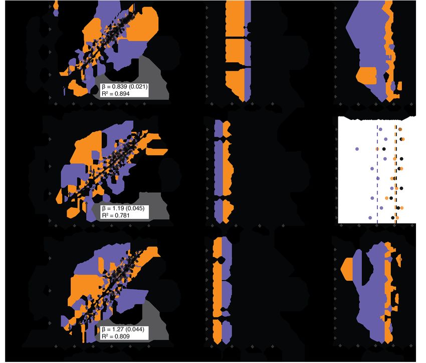
FIG. 1. Spatio-temporal dynamics of population. a, b, The spatial distributions of daytime
(a) and nighttime (b) population for Beijing. c, The daytime, nighttime, and active population
density gradients from the city center to the periphery for Beijing.

   RESULTS

   Active population

   To incorporate the temporal dynamics and derive a better measure of the population
distribution, we employ the concept of the active population (AP), which is a more appro-
priate proxy than simply residential or employment population for estimating socioeconomic
activity [5]. The AP reflects a mixture of the daytime and nighttime populations within a
given region by combing them together with the active time as a weight λ:

                            AP = λDayP opu + (1 − λ)N ightP opu.                           (1)

   Here, the daytime and nighttime populations are estimated by a large-scale mobile phone
dataset for the year 2015 (see Fig. 1a, b and Methods for details). For the ten cities studied,
we have a total of 107 million mobile phone users (see Supplementary Table 1 for details).
   The total AP in one city is the same as the total daytime or nighttime population if
there is no intercity commuting. Stated simply, we further assume that the duration of
daytime and nighttime is approximately 1:1, i.e., 12 hours for daytime and 12 hours for
nighttime in one day. Therefore, we have λ = 1/2 in Eq. (1). In other words, here we use
the average of the daytime and nighttime population as a measure of the AP. One benefit
of this setting is that for cities without mobile phone data, AP could be calculated by the
employment (daytime) and residential (nighttime) populations, which are available in many

                                                4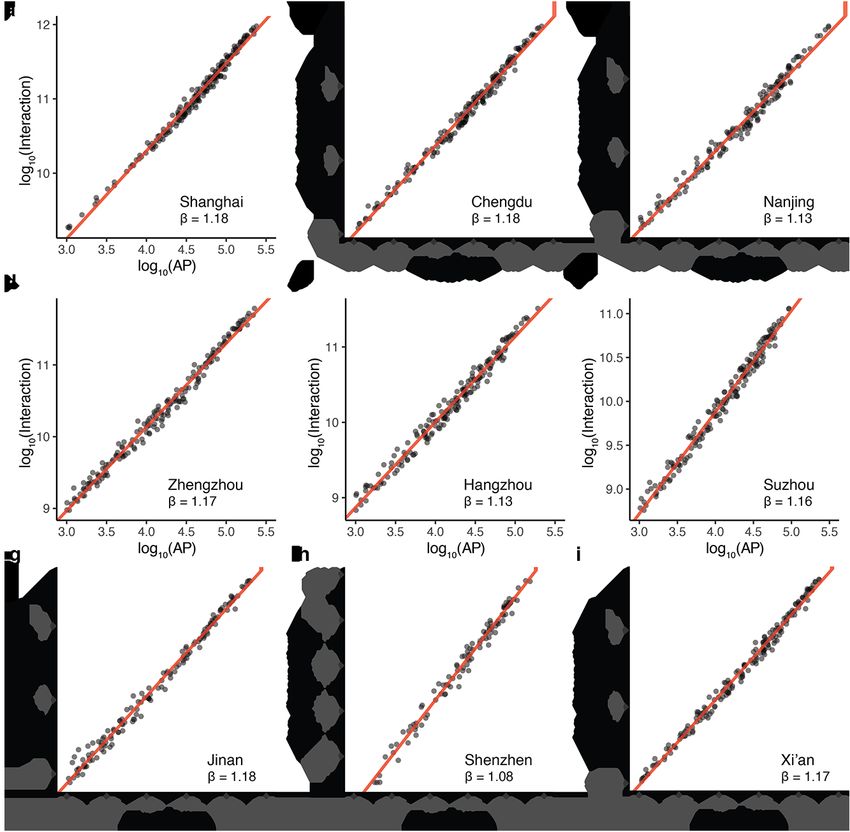
cities’ official statistics. In Supplementary Fig. 2, we further show the results by adjusting
λ, and all conclusions are robust.
   We present the daytime, nighttime, and active population density gradients from the
downtown to the urban fringe of Beijing in Fig. 1c. Previous studies have found that
population density decays from the city center with an exponential, power-law-like, or some
more complex forms [33]. We find similar patterns in the granular population data. The
population density curves, however, vary significantly between day and night especially
around the urban core areas as shown in Fig. 1c.

   The empirical findings

   Given the detailed spatial distributions of urban elements, a proper spatial unit is then
required to perform the statistical analysis. In order to make the results of different cities
comparable, here we use a 2km×2km grid as our analysis units (see Methods for details). To
address the potential modifiable areal unit problem (MAUP), meaning the statistical results
are influenced by the scale of the aggregation unit [34, 35], we also perform a robustness
check by varying the size of the grid, all results are stable (Supplementary Table 2).
   We aggregate the daytime/nighttime/active populations, buildings, firms, and POIs into
the corresponding grid cell. To derive the scaling exponent, we take the simplest fitting
procedure, minimizing ordinary least squares (OLS) to a linear relation of the logarithmic
variables:

                              log10 Yi = log10 Y0 + β log10 Pi + i ,                        (2)

where i indexes different grid cells in a city, the dependent variable Yi denotes the infras-
tructure volume, the number of firms, or the number of POIs, and Pi is the population size.
i is the error term.
   The fitting results between population and infrastructure volume are shown in Fig. 2a-c.
Here we use the total building areas (i.e., building volumes) to represent the infrastructure
volume by assuming a linear relationship between them (for example, one elevator services
a certain amount of building areas in office buildings or in apartments). Figure 2b shows
that in all studied cities, the scaling exponents of infrastructure are less than 1, indicating a
robust sub-linear relationship with the population size. Interestingly, the average value (over

                                               5
FIG. 2. Intra-urban scaling of infrastructure and socioeconomic interactions. a-c, The
sub-linear scaling between population and infrastructure volume. d-i, The super-linear scaling
between population and the number of firms (d-f) and the number of POIs (g-i). a, d, g, The
scatter plots and fitting results of Beijing for the infrastructure volume (a), the number of firms
(d), and the number of POIs (g). b, e, h, The scaling exponents (± one standard error) of ten
studied cities. c, f, i, R2 of daytime, nighttime, and active populations. The mean values of β and
R2 are labeled with dashed lines.
all cities) hβinf ra i ≈ 0.833 being very close to 5/6, a theoretical value of the scaling exponent
between infrastructure and population across cities [3]. Moreover, Figure 2c clearly shows
that compared with daytime and nighttime populations, the AP achieves the highest R2 in
2
all cities (hRinf ra|ap i ≈ 0.839), which demonstrates the effectiveness of the AP measurement.
6To investigate the super-linear scaling within cities, we collect two granular socioeconomic
activity datasets: the firm registration record data and the POI data (see Methods). We
use the number of firms and POIs as the proxy variables for socioeconomic activity. Figure
2eh shows that the super-linear scaling between AP and socioeconomic activity holds well in
both datasets. In all ten cities, the scaling exponents of firms and POIs are both greater than
1 and the average value is approximately 1.25, which is very close to the empirical results
across cities and the theoretical values of 7/6 [3] or 4/3 [36] derived from different models.
Similar to the infrastructure results, the R2 calculated by the AP is the highest in most cities
(Fig. 2fi). We notice that for the firm dataset the daytime population also performs well
in terms of the R2 . This is not difficult to understand, as most firm-related activities occur
during the day and are closely related to the daytime population (employment) distribution.
Despite the robust sub/super-linear relationships, we can also observe differences in the
scaling exponents as shown in Fig. 2. Specifically, for a same scaling phenomenon, the
scaling exponents of cities with similar population sizes can be statistically different. For
instance, the population of Shenzhen and Xi’an is similar (between 12 and 13 million), but
the exponents of infrastructure, number of firms and POIs in the two cities are significantly
different (Fig. 2). A similar pattern is found in the data of Beijing and Shanghai (population
is between 22 and 24 million), firms scale more superlinearly in Shanghai compared with
Beijing (Fig. 2e). These findings suggest that population size is not the only determining
parameter that influences the scaling phenomena within cities.
The conceptual framework
To explain these empirical observations simultaneously we propose a conceptual frame-
work. The main ideas are that the two key elements that constitute a city, its physical
infrastructure and socioeconomic activity, can be modeled by the local and global spatial
interactions with its citizens, respectively; and the interaction intensity has a city-specific
parameter. The sub-linear scaling is derived by the local interactions between population
and infrastructure (Fig. 3a), because the infrastructure networks develop in a decentralized
way in order to connect people, which is also a main assumption in Bettencourt’s model [3].
The super-linear scaling is assumed to be the results of global interactions between popula-
tion (Fig. 3d). All of our analyses below consider the heterogeneous population distribution,
7FIG. 3. The sub-linear relationship. a, Illustration of the localized connection between AP and
infrastructure. We assume that an AP connects to its n nearest neighbors by the infrastructure
network, and n is a constant number. Note that A is calculated by summing up the footprint area
of each building in a given cell, and A varies across cells. b, c, Scaling relation ` ∼ ρ−α of empirical
data (b) [α = 0.562(0.016), R2 = 0.985] and simulated data (c) [α = 0.448(0.013), R2 = 0.970]. d,
Illustration of the global interaction between people and people. e, Scatter plots of 1 − α and α,
which are the exponents of P and A in the regression log10 Ii = log10 I0 +(1−α) log10 Pi +α log10 Ai ,
respectively. The red line is the prediction of the Cobb-Douglas function with constant returns to
scale. f, R2 s of the ten studied cities. The average R2 obtained from Eq. (4) is 0.927 (red dots),
and we also put the results of Fig. 2c here (black dots) for comparison.
and this goes beyond previous theoretical frameworks [3, 19].
Let ρi denote the population density of cell i, and ρi = Pi /Ai , where Pi is the active
population size and Ai is the building footprint area within cell i (gray areas in Fig. 4a).
Since infrastructure services population in a localized way, we assume that the typical length
of infrastructure (e.g., roads, pipes, and cables) ` depends on ρ in the following form
8` ∼ ρ−α , (3)
where α (0 < α < 1) is a city-specific parameter controlling the local interaction intensity.
This equation can be verified with both empirical and simulated data as shown in Fig.
3bc. Empirically, we collect city level road network data from Ref. [37], which includes
twenty 1 square mile samples of different world cities. Figure 3b shows that the relationship
between the average road length ` and the density of road intersections is well-fitted by Eq.
(3) (α = 0.562, R2 = 0.985). As shown in Ref. [38], the number of road intersections is
proportional to the population size, thus the density of road intersections can be a proxy
for population density ρ. Simulation experiments also support Eq. (3). We generate 20,000
points under a two-dimensional Gaussian distribution within an L × L space, connect each
point to its n (n = 3) nearest neighbor, and calculate the relation between point density ρ
and average edge length ` by L/10 × L/10 grid cells. The fitting results are α = 0.448 and
R2 = 0.970, respectively.
The total infrastructure length Ii within cell i is thus given by the production of the
population Pi and the average infrastructure length `i
Ii = `i Pi ∼ Pi1−α Aαi . (4)
This equation means that the larger the α, the smaller/larger the impact of the population
P /footprint area A on the infrastructure. We notice that Eq. (4) is a special case of the
Cobb-Douglas production function [12, 39], which displays constant returns to scale as the
sum of the exponents equals 1 (1 − α + α ≡ 1). The constant returns to scale means that
doubling the population P and footprint area A will also double infrastructure I. We take
the logarithm of Eq. (4), and perform a simple OLS regression to estimate the coefficients –
1 − α and α – for each city. As shown in Fig. 3e, the exponents of P and A of different cities
almost perfectly fall on the predicted line given by the constant returns to scale property.
The values of α in most cities is approximately 0.7, but Beijing and Chengdu are smaller,
approximately 0.35.
The analytical and empirical results of Eq. (4) imply that both population and foot-
print area can contribute to infrastructure volume, which is rarely mentioned in the scaling
literature. In other words, population is not the only determining factor that affects the in-
9frastructure within cities (similarly, Ref. [12] finds that population and built-up area jointly
affect the urban carbon dioxide emissions). Take some newly developed areas in a city for
example, the population size of these areas has not yet grown, therefore the infrastructure
volume of these areas is much higher than the value predicted by the current population.
A similar issue exists for urban slums, where the infrastructure is much lower than the
predicted number based on their population size. These intra-urban variations in land use
partially explain why the data points shown in Fig. 2 are much noisier than the cross-city
plots. By considering both P and A we can obtain a better fitting result for infrastructure,
and the average R2 increases from 0.839 to 0.927 (Fig. 3f).
Although P , A, and I are coupled together as shown in Eq. (4), we can still obtain a
simple scaling exponent between P and I by assuming a power-law relationship between P
and A. In Supplementary Fig. 3, we empirically show that A ∼ P η (hηi ≈ 0.734 < 1).
Thus, we obtain
1−α(1−η)
Ii ∼ Pi . (5)
The exponent βsub = 1 − α(1 − η) is less than 1, indicating a sub-linear scaling. The
tunable parameters α and η capture the heterogeneity in different cities.
Unlike sub-linear scaling, we argue that the super-linear scaling within cities is the result
of global (i.e., city-wide) interactions between people (Fig. 3d). To model the global inter-
actions, we employ the gravity function, which is widely used to mimic the interaction flows
(e.g., people, goods) between different regions [40–42]. This practice also links urban scaling
to human mobility, as the gravity model is one of the most important mobility models.
Let fij denote the interaction between cell i and j, according to the gravity function, we
have
kPi Pj
fi = , (6)
dγij
where dij is the Euclidean distance between the centroid of cell i and j, γ is a parameter
controlling the geographical constrain for the interaction, and k is the constant. This equa-
tion includes two effects for interactions: i) the active population Pi captures the preferential
attachment meaning a popular location will attract more people; ii) dγij captures the spatial
dependence. Here, γ = 1 is particularly noteworthy because of γ = 1 exactly corresponding
to the gravity field in a two-dimensional space (γ = 2 corresponds to the classic Newton’s
10law of gravitation in a three-dimensional space) [43], and the model becomes a ‘parameter-
free’ model under this setting. Experimentally, the value of γ ranges in the interval [1, 1.5]
[44–47].
Fi , the total interactions of location i, can be derived by summing Eq. (6):
X Pj
Fi = kPi . (7)
dγ
j6=i ij
Due to the complicated spatial correlation between Pj and dij , there is no general ana-
lytical solution for Fi , here we present the numerical estimations based on the population
distribution of the studied cities. Figure 4a show interactions Fi as a function of the active
population size Pi for Beijing (see Supplementary Fig. 4 for the results of the remaining
cities). As can be seen, all data points fall almost exactly on a straight line with a slope
greater than one, indicating that the gravity function can effectively reproduce the super-
linear scaling between population and interactions. More importantly, we find that βsup
derived by our ‘parameter-free’ model (γ = 1) is very close to the theoretical value 7/6
across cities [3], which provides some new insights into the long-standing debate over the
gravity model coefficients in urban fields [48].
Figure 4b further shows that the scaling exponent βsup increases monotonically as γ
increases, and βsup ranges from 1.15 to 1.34 when γ ranges from 1 to 2. And we find a linear
relationship between γ and βsup within this range:
βsup ≈ a + b(γ − 1), (8)
where a = 1.153 (0.001) and b = 0.186 (0.000) (R2 = 0.999 and p-value = 1.288 ×10⁻⁹ ). βsup
derived from the model is quite similar to our empirical findings (see Fig. 2, we assume the
number of firms and POIs is proportional to the volume of interactions). Also, the tunable
parameter γ reflects the variations of global interaction in different cities and different urban
phenomena.
Spatial autocorrelation, gravity, and super-linear scaling
We notice that the population distributions of different cities fluctuate greatly (Supple-
mentary Fig. 1), but all cities have similar super-linear scaling exponents under the same γ
11FIG. 4. Gravity model, Moran’s I, and the super-linear scaling. a, Scatter plots and fitting
results between AP and gravity-based interactions for Beijing (γ = 1). b, Urban scaling exponent
βsup changes with the values of γ. The mean values of βsub (y-axis) were calculated based on the
simulation results of the ten studied cities (with ± one standard deviation). Interestingly, we find
a linear relationship between γ and βsup when γ ranges from 1 to 2 (the red line), and the cases
γ = 1 and 2 effectively reproduce the theoretical estimations of β = 7/6 and 4/3, respectively. c,
The super-linear scaling between interaction and the number of nodes (population) with σ = 1
and γ = 1. d, Relation between Moran’s I and the scaling exponent β. β increases monotonically
as Moran’s I increases, and the theoretical value β = 7/6 corresponds to Moran’s I = 0.66, the
similar value to the empirical results of Moran’s I.
(Supplementary Fig. 4). It is supposed that there should be some unified hidden parame-
ters behind the spatial distribution of population contributing to the universal super-linear
scaling behaviors. Spatial autocorrelation is a good candidate for that parameter under the
12Exponents Within cities Across cities
Observation Model Observation Model
βsub [0.70,0.92] 1 − α(1 − η) [0.74,0.92] 1−δ
βsup [1.07,1.41] a + b(γ − 1) [1.01,1.33] 1+δ
TABLE I. Scaling exponents within cities and across cities
Note: the empirical and theoretical results across cities are obtained from Ref. [3].
intra-urban setting, because most geographical phenomena have positive spatial autocorre-
lation and dependence [49], and people in cities also form spatial dependent communities
(or clusters). To test this assumption, we calculate Moran’s I [50], the most commonly used
indicator for spatial autocorrelation, and show the connection between Moran’s I and the
scaling exponent (see Methods).
Empirically, we find that the value of Moran’s I of the active population distribution
is mostly between 0.55 and 0.75 (Supplementary Table 3), implying that different cities
have similar spatial autocorrelation patterns in terms of population distribution. Since the
difference in the values of Moran’s I between different cities is small, we cannot directly test
the relationship between Moran’s I and super-linear scaling through empirical data. So we
conduct a series of numerical simulations to generate point patterns with different Moran’s
Is. We generate 1 × 10⁵ points under a two-dimensional Gaussian distribution with the
mean µ = 0 and the standard deviation σ varying from 0.25 to 4. We then partition the
space by 0.5 × 0.5 grid cells and calculate the interaction between each cell pair based on the
gravity equation (γ = 1). For each σ, we run thirty simulations and take the average values
of σ and β. We highlight two empirical findings: 1) the simulated point distribution and
gravity equation effectively resemble the super-linear scaling patterns and exponents (Fig.
4c). 2) β increases monotonically as Moran’s I increases, and the theoretical value β = 7/6
corresponds to Moran’s I = 0.66 (Fig. 4d), the similar value to the empirical results of ten
cities (Supplementary Table 3). All these findings point to a promising direction to study
the in-depth connection between spatial patterns and scaling phenomena.
13DISCUSSION
In summary, we analyzed a diverse set of extensive urban data, and find that cities
exhibit robust intra-urban power-law scaling at the mesoscopic level: the infrastructure and
socioeconomic activity satisfy sub- and super-linear exponents, respectively. Because the size
of grid cells used here is somewhat arbitrary, we perform a sensitivity analysis by varying
the cell size, all conclusions are robust (Supplementary Table 2). Notably, the average intra-
urban scaling exponents are consistent with previous cross-city results, providing direct
empirical support to the hypothesis that cities are self-similar [32] and manifest power-
law scaling inside themselves as well. This finding also echoes the fractal nature of urban
systems.
To explain the observed regularity and heterogeneity in the mesoscopic scaling phenom-
ena, we provide a conceptual framework by decomposing spatial interactions into local and
global effects. The sub-linear scaling of infrastructure volume can be derived through the
local effect and is found to be jointly influenced by population and footprint areas. The
super-linear scaling is attributed to the city-wide interactions, which links urban super-
linear scaling to human mobility. By adjusting the city-specific parameters α, η, and γ, we
give a better description of the real world, where the scaling exponents do not always appear
symmetrically as β = 1 ± δ for super- and sub-linear scaling predicted by previous models
(Table I). In particular, there is always a higher exponent for some super-linear scaling phe-
nomena such as innovation and epidemic spreading [1]; this may be primarily due to these
phenomena being affected more by global interactions (a larger γ or a more autocorrelated
population distribution).
It is important to note that, due to the accessibility of the dataset, we only present the
results from ten large Chinese cities with high population density. Further research is needed
to show whether the revealed patterns hold in other configurations, such as a spatially
constrained city like Seattle or San Francisco, or a city whose growth has been largely
uncontrolled, such as Los Angeles or Mexico City. Also, because our framework is minimal,
it ignores various factors, such as transportation investment, policy, geographical barriers, all
of which could affect the distribution of urban elements and the studied scaling phenomena.
However, this paper provides an empirical and theoretical basis, where additional data and
factors can be incorporated.
14METHODS
Population distribution dataset. The population distribution is estimated by a large-
scale mobile phone dataset, which is provided by one location-based service provider in
China. The mobile phone data have been used in our previous studies [51, 52], and the
population coverage of this dataset is shown in Supplementary Table 1. To protect user’s
privacy, we adopt very rigorous protocol in this research. Firstly, all user IDs in our data
are hashed and anonymized to ensure that one cannot associate the data to individual users.
Secondly, all the researchers must follow a confidential agreement to use data for approved
research. Thirdly, we solely focus on aggregated instead individual level to perform the
scaling analysis in this research.
To estimate the daytime and nighttime population distributions, we take the following
steps:
• i) Detecting stay point. For each anonymous individual, we have a series of geo-
positiong points {timestamp, longitude, latitude}. A stay point is defined by a moving
distance less than d = 200m meters within a t = 10min minute time threshold. As
documented in our previous research [51], the stay points are robust when adjusting
these thresholds within reasonable ranges.
• ii) Clustering. We cluster the stay points into different clusters using the DBSCAN
algorithm [53]. These clusters are defined as the stay locations.
• iii) Classification. We extract 28 features from the data (see Supplementary Table
4 for the main features). Then, we use Xgboost [54], a supervised machine learning
algorithm, to train two classifiers for the work and home location classification, re-
spectively. The classification models are trained with a dataset that with the labels
of home and work (ground truth). The distributions of work and home locations are
regarded as the daytime and nighttime population distributions, respectively. Fig.
1ab present the spatial distributions of detected home and work locations of Beijing.
To verify the accuracy of the results, we calculate the correlation between mobile phone
inferred home locations and the micro-census data of the year 2015 (the same year of our mo-
bile phone dataset) at the district level. The R2 s of the linear regression (log M obileP hone =
15β log Survey +) are 0.97 for Beijing and 0.98 for Shanghai, indicating that the mobile phone
estimated population has good consistency with the survey data in terms of geographical
distribution (Supplementary Fig. 5). The correlation between mobile phone data and offical
statistics has also been discussed in the studies of Estonia [55], Portugal [27], and France
[56].
Building dataset. The building data were collected from one digital map in China.
The original records were labeled based on various data sources, including remote sensing,
streetview imagery, and LiDAR. The geographical layouts of the buildings are presented
in Supplementary Fig. 1 and Supplementary Fig. 6. We should note that since there is
no ground truth for the building dataset, we cannot directly measure its quality. But in
Ref. [57], researchers from Microsoft track some metrics to measure the quality of a similar
building dataset in the US. The IoU (intersection over union) of that test set is 0.85.
Firm dataset. We collected firm registration record data from the registry database of
the State Administration for Industry and Commercial Bureau of China. This dataset covers
the registered information for all firms in China, with attributes including firm name, year
established, address, operation status, and so on. We geocode firm addresses into longitude
and latitude and then aggregate firms by grid cells of each city. Two limitations of the firm
data should be noted: firstly, we only have registered address, which may not be the same as
the operation address; and secondly, firm size (e.g., the number of employees or the revenue)
is unreported in the raw dataset.
POI dataset. We collected POI data from dianping.com, the largest online rating
website in China. The raw data include detailed locations of restaurants, shops, and service
businesses (e.g., hair salon, photo studio), here we use points of restaurants and shops for
our analysis. We note that the penetration rates of dianping.com in these two categories
are high implying that the scaling exponent is less likely to be affected by the sample
bias. For example, according to a report by Beijing Cuisine Association, there were 147,575
restaurants in operation at the end of 2016. In our dataset, we have 139,131, which covers
94.3% of the total number of restaurants.
Threshold. To make the results comparable across cities, we restrict all our data and
analysis within the urban core area (the distance from the city center ≤ 15km for Beijing
and ≤ 10km for the remaining cities. The coordinates of the city center are presented in the
third column of Supplementary Table 1). To reduce the potential noise in the datasets, we
16further set four thresholds – 10−2 km2 for footprint area, 1,000 for mobile phone estimated
population, 2 for the number of firm, and 2 for the number of POIs – to remove cells with
values less than the thresholds. The number of cells used in the regression is shown in the
second column of Supplementary Table 1.
Grid cell. We transform the coordinate of each data point from World Geodetic System
1984 longitude and latitude to a projected system (Gauss-Kruger) and build the grid system.
For the grid cell division, we have two further explanations. The first is about the modifiable
areal unit problem. With this grid style division, we can use different cell sizes to verify
the robustness of the conclusions, which we have discussed in the Discussion section and
Supplementary Table 2. The second point is about a fundamental question – how to define
a city. Undoubtedly, a city is composed of a series of sub-units. According to the theory
of fractal cities or hierarchical network-embedded cities, we have reason to find self-similar
units within cities. This kind of grid cell division provides a basis for us to find such a unit.
Specifically, the 2km × 2km grid corresponds to the typical activity range of people’s daily
life, which is equivalent to a 15min living circle (people walk at a speed of 4-5km per hour).
Moran’s I. To calculate Moran’s I, we use the following formula:
Pn Pn
n i=1 wij zi zj
MI = Pnj=1 2 , (9)
W i=1 zi
where n is the number of observations (grid cells in our case), W is the sum of the weights
wij for all cell pairs in a city, zi = xi − x̄ where x is the active population size at location
i and x̄ is the mean active population size in the city. Moran’s I has a value from -1 to
1: -1 means perfect clustering of dissimilar values (i.e., perfect dispersion); 0 indicates no
autocorrelation (i.e., perfect randomness); and 1 indicates perfect clustering of similar values
(opposite of dispersion).
Acknowledgements
We thank Micheal Goodchild and seminar participants at Peking University for helpful
discussions. This research was supported by the National Natural Science Foundation of
China (no. 41801299) and the China Postdoctoral Science Foundation (no. 2018M630026).
17Author contributions
L.D., Z.H., J.Z., and Y.L. designed research; L.D. performed research; L.D., J.Z., and
Y.L. analyzed data; L.D. and Y.L. wrote the paper.
Data and code availability
Data and code necessary to reproduce our results are available through https://github.
com/leiii/MesoScaling.
Competing interests
The authors declare no competing financial interests.
[1] Luı́s MA Bettencourt, José Lobo, Dirk Helbing, Christian Kühnert, and Geoffrey B West.
Growth, innovation, scaling, and the pace of life in cities. Proceedings of the National Academy
of Sciences, 104(17):7301–7306, 2007.
[2] Luı́s MA Bettencourt and Geoffrey West. A unified theory of urban living. Nature,
467(7318):912, 2010.
[3] Luı́s MA Bettencourt. The origins of scaling in cities. Science, 340(6139):1438–1441, 2013.
[4] Rémi Louf and Marc Barthelemy. How congestion shapes cities: From mobility patterns to
scaling. Scientific Reports, 4:5561, 2014.
[5] Ruiqi Li, Lei Dong, Jiang Zhang, Xinran Wang, Wen-Xu Wang, Zengru Di, and H Eugene
Stanley. Simple spatial scaling rules behind complex cities. Nature Communications, 8(1):1841,
2017.
[6] Andres Gomez-Lievano, Oscar Patterson-Lomba, and Ricardo Hausmann. Explaining the
prevalence, scaling and variance of urban phenomena. Nature Human Behaviour, 1(1):0012,
2017.
[7] Hyejin Youn, Luı́s MA Bettencourt, José Lobo, Deborah Strumsky, Horacio Samaniego, and
Geoffrey B West. Scaling and universality in urban economic diversification. Journal of The
Royal Society Interface, 13(114):20150937, 2016.
18[8] Michael Batty. The size, scale, and shape of cities. Science, 319(5864):769–771, 2008.
[9] Horacio Samaniego and Melanie E Moses. Cities as organisms: Allometric scaling of urban
road networks. Journal of Transport and Land Use, 1(1):21–39, 2008.
[10] Michael Batty. The New Science of Cities. MIT Press, 2013.
[11] Marc Barthelemy. The Structure and Dynamics of Cities. Cambridge University Press, 2016.
[12] Haroldo V Ribeiro, Diego Rybski, and Jürgen P Kropp. Effects of changing population or
density on urban carbon dioxide emissions. Nature Communications, 10, 2019.
[13] Marcus J Hamilton, Bruce T Milne, Robert S Walker, and James H Brown. Nonlinear scaling
of space use in human hunter–gatherers. Proceedings of the National Academy of Sciences,
104(11):4765–4769, 2007.
[14] Scott G Ortman, Andrew HF Cabaniss, Jennie O Sturm, and Luı́s MA Bettencourt. Settle-
ment scaling and increasing returns in an ancient society. Science Advances, 1(1):e1400066,
2015.
[15] Peter Hall. Cities of tomorrow: An intellectual history of urban planning and design since
1880. John Wiley & Sons, 2014.
[16] Gabriel M Ahlfeldt and Elisabetta Pietrostefani. The economic effects of density: A synthesis.
Journal of Urban Economics, 111:93–107, 2019.
[17] Darren Timothy and William C Wheaton. Intra-urban wage variation, employment location,
and commuting times. Journal of Urban Economics, 50(2):338–366, 2001.
[18] Gilles Duranton and Diego Puga. Micro-foundations of urban agglomeration economies. In
Handbook of Regional and Urban Economics, volume 4, pages 2063–2117. Elsevier, 2004.
[19] Wei Pan, Gourab Ghoshal, Coco Krumme, Manuel Cebrian, and Alex Pentland. Urban
characteristics attributable to density-driven tie formation. Nature Communications, 4:1961,
2013.
[20] Jaegon Um, Seung-Woo Son, Sung-Ik Lee, Hawoong Jeong, and Beom Jun Kim. Scaling laws
between population and facility densities. Proceedings of the National Academy of Sciences,
106(34):14236–14240, 2009.
[21] Marc Keuschnigg, Selcan Mutgan, and Peter Hedström. Urban scaling and the regional divide.
Science Advances, 5(1):eaav0042, 2019.
[22] Marc Keuschnigg. Scaling trajectories of cities. Proceedings of the National Academy of
Sciences, page 201906258, 2019.
19[23] Jules Depersin and Marc Barthelemy. From global scaling to the dynamics of individual cities.
Proceedings of the National Academy of Sciences, 115(10):2317–2322, 2018.
[24] Fabiano L. Ribeiro, Joao Meirelles, Vinicius M. Netto, Camilo Rodrigues Neto, and Andrea
Baronchelli. On the relation between transversal and longitudinal scaling in cities. arXiv,
page 1910.02113, 2019.
[25] Luis Bettencourt, Vicky Chuqiao Yang, José Lobo, Chris Kempes, Diego Rybski, and Marcus
Hamilton. The interpretation of urban scaling analysis in time. Mansueto Institute for Urban
Innovation Research Paper Forthcoming, 2019.
[26] Deborah Strumsky, Jose Lobo, and Charlotta Mellander. As different as night and day: Scaling
analysis of swedish urban areas and regional labor markets. Environment and Planning B:
Urban Analytics and City Science, page 2399808319861974, 2019.
[27] Pierre Deville, Catherine Linard, Samuel Martin, Marius Gilbert, Forrest R Stevens, Andrea E
Gaughan, Vincent D Blondel, and Andrew J Tatem. Dynamic population mapping using
mobile phone data. Proceedings of the National Academy of Sciences, 111(45):15888–15893,
2014.
[28] Michael Batty, Rui Carvalho, Andy Hudson-Smith, Richard Milton, Duncan Smith, and Philip
Steadman. Scaling and allometry in the building geometries of greater london. The European
Physical Journal B, 63(3):303–314, 2008.
[29] Markus Schläpfer, Joey Lee, and Luı́s MA Bettencourt. Urban skylines: building heights and
shapes as measures of city size. arXiv preprint arXiv:1512.00946, 2015.
[30] Crocker H Liu, Stuart S Rosenthal, and William C Strange. The vertical city: Rent gradients,
spatial structure, and agglomeration economies. Journal of Urban Economics, 106:101–122,
2018.
[31] Elsa Arcaute, Erez Hatna, Peter Ferguson, Hyejin Youn, Anders Johansson, and Michael
Batty. Constructing cities, deconstructing scaling laws. Journal of The Royal Society Interface,
12(102):20140745, 2015.
[32] Michael Batty and Paul A Longley. Fractal cities: a geometry of form and function. Academic
Press, 1994.
[33] Joan Carles Martori, Rafa Madariaga, and Ramon Oller. Real estate bubble and urban pop-
ulation density: six spanish metropolitan areas 2001–2011. The Annals of Regional Science,
56(2):369–392, 2016.
20[34] S Openshow and P Taylor. A million or so correlation coefficients, three experiments on the
modifiable areal unit problem. Statistical Applications in the Spatial Science, pages 127–144,
1979.
[35] Rémi Louf and Marc Barthelemy. Scaling: lost in the smog. Environment and Planning B:
Planning and Design, 41(5):767–769, 2014.
[36] Jiang Zhang, Xintong Li, Xinran Wang, Wen-Xu Wang, and Lingfei Wu. Scaling behaviours
in the growth of networked systems and their geometric origins. Scientific Reports, 5:9767,
2015.
[37] Alessio Cardillo, Salvatore Scellato, Vito Latora, and Sergio Porta. Structural properties of
planar graphs of urban street patterns. Physical Review E, 73(6):066107, 2006.
[38] Emanuele Strano, Vincenzo Nicosia, Vito Latora, Sergio Porta, and Marc Barthélemy. Ele-
mentary processes governing the evolution of road networks. Scientific Reports, 2:296, 2012.
[39] Charles W Cobb and Paul H Douglas. A theory of production. American Economic Review,
18(1):139–165, 1928.
[40] Marko Popović, Hrvoje Štefančić, and Vinko Zlatić. Geometric origin of scaling in large traffic
networks. Physical Review Letters, 109(20):208701, 2012.
[41] Diego Rybski, Anselmo Garcia Cantu Ros, and Jürgen P Kropp. Distance-weighted city
growth. Physical Review E, 87(4):042114, 2013.
[42] K Yakubo, Y Saijo, and D Korošak. Superlinear and sublinear urban scaling in geographical
networks modeling cities. Physical Review E, 90(2):022803, 2014.
[43] Mattia Mazzoli, Alex Molas, Aleix Bassolas, Maxime Lenormand, Pere Colet, and José J
Ramasco. Field theory for recurrent mobility. Nature communications, 10(1):1–10, 2019.
[44] Pierre Deville, Chaoming Song, Nathan Eagle, Vincent D Blondel, Albert-László Barabási, and
Dashun Wang. Scaling identity connects human mobility and social interactions. Proceedings
of the National Academy of Sciences, 113(26):7047–7052, 2016.
[45] Yu Liu, Chaogui Kang, Song Gao, Yu Xiao, and Yuan Tian. Understanding intra-urban trip
patterns from taxi trajectory data. Journal of Geographical Systems, 14(4):463–483, 2012.
[46] Fabiano L Ribeiro, Joao Meirelles, Fernando F Ferreira, and Camilo Rodrigues Neto. A model
of urban scaling laws based on distance dependent interactions. Royal Society Open Science,
4(3):160926, 2017.
21[47] Anne-Célia Disdier and Keith Head. The puzzling persistence of the distance effect on bilateral
trade. The Review of Economics and Statistics, 90(1):37–48, 2008.
[48] Filippo Simini, Marta C González, Amos Maritan, and Albert-László Barabási. A universal
model for mobility and migration patterns. Nature, 484(7392):96, 2012.
[49] Luc Anselin. Spatial econometrics. A Companion to Theoretical Econometrics, 310330, 2001.
[50] Patrick AP Moran. Notes on continuous stochastic phenomena. Biometrika, 37(1/2):17–23,
1950.
[51] Lei Dong, Sicong Chen, Yunsheng Cheng, Zhengwei Wu, Chao Li, and Haishan Wu. Measuring
economic activity in China with mobile big data. EPJ Data Science, 6(1):29, 2017.
[52] Lei Dong, Carlo Ratti, and Siqi Zheng. Predicting neighborhoods socioeconomic attributes
using restaurant data. Proceedings of the National Academy of Sciences, 116(31):15447–15452,
2019.
[53] Martin Ester, Hans-Peter Kriegel, Jörg Sander, and Xiaowei Xu. A density-based algorithm
for discovering clusters in large spatial databases with noise. In Proceedings of the Second
International Conference on Knowledge Discovery and Data Mining, pages 226–231. AAAI
Press, 1996.
[54] Tianqi Chen and Carlos Guestrin. Xgboost: A scalable tree boosting system. In Proceedings of
the 22nd International Conference on Knowledge Discovery and Data Mining, pages 785–794.
ACM, 2016.
[55] Rein Ahas, Siiri Silm, Olle Järv, Erki Saluveer, and Margus Tiru. Using mobile positioning
data to model locations meaningful to users of mobile phones. Journal of Urban Technology,
17(1):3–27, 2010.
[56] Maarten Vanhoof, Fernando Reis, Thomas Ploetz, and Zbigniew Smoreda. Assessing the
quality of home detection from mobile phone data for official statistics. Journal of Official
Statistics, 34(4):935–960, 2018.
[57] US Building Footprints. https://github.com/Microsoft/USBuildingFootprints. Ac-
cessed: 2018-12-30.
22Supplementary Information
SUPPLEMENTARY TABLES
City N Center (lat., lon.) Population (104 ) Mobile Phone Data Coverage (%)
Beijing 198 39.907, 116.391 2,171 77.2
Shanghai 94 31.231, 121.471 2,415 63.2
Chengdu 96 30.659, 104.064 1,466 74.0
Nanjing 77 32.043, 118.779 823 63.7
Zhengzhou 86 34.747, 113.654 957 75.2
Hangzhou 59 30.242, 120.204 902 72.0
Suzhou 57 31.302, 120.581 1,062 81.7
Jinan 57 36.672, 116.989 700 54.9
Shenzhen 39 22.540, 114.060 1,303 111*
Xi’an 63 34.261, 108.942 871 84.4
Supplementary Table 1 Descriptive statistics of ten cities. N is the number of grid cells
used in the analysis. The coordinates of urban center are collected from Wikipedia; population
size is derived from the city yearbook. The mobile phone data coverage equals our mobile phone
samples divided by the urban population. *: Because Shenzhen has a large number of floating
population making the official statistics of the population underestimate the actual size of the
population. This is why we find that the number of mobile phone users is higher than the official
urban population.
232
Cell size hβinf ra i hRinf 2 2
ra i hβf irm i hRf irm i hβP OI i hRP OI i
1km 0.753 0.745 1.29 0.730 1.25 0.738
1.5km 0.799 0.816 1.26 0.793 1.25 0.783
2.5km 0.854 0.891 1.24 0.858 1.27 0.862
Supplementary Table 2 Cell sizes and scaling results. All values are averaged for ten
studied cities.
City Moran’s I
Beijing 0.649
Shanghai 0.676
Chengdu 0.716
Nanjing 0.588
Zhengzhou 0.703
Hangzhou 0.556
Suzhou 0.558
Jinan 0.740
Shenzhen 0.344
Xi’an 0.719
Supplementary Table 3 Moran’s I. To calculate the Moran’s I of the spatial distribution of
active population, we use the lctools package
(https://cran.r-project.org/web/packages/lctools/index.html) in R.
24Category Feature
Individual level # of stay point
# of unique date of stay point
weekday # of stay point / weekend # of stay point
weekday daytime # of stay point / weekday nighttime # of stay point
Cluster level weekday # of stay point / weekend # of stay point (each cluster)
weekday daytime # of stay point / weekday nighttime # of stay point (each cluster)
# of stay point in each cluster / total # of stay point
weekday # of stay point (each cluster) / total # of stay point
weekend # of stay point (each cluster) / total # of stay point
daytime # of stay point (each cluster) / total # of stay point
nighttime # of stay point (each cluster) / total # of stay point
# of other clusters to this cluster before 12:00 (transfer matrix)
# of this cluster to other cluster before 12:00 (transfer matrix)
# of other clusters to this cluster after 12:00 (transfer matrix)
# of this cluster to other cluster after 12:00 (transfer matrix)
Regional level Region ID
POI level # of residential point of interests (POI)
# of working point of interests (POI)
Supplementary Table 4 Main features for home and work location
classification. We set 9:00-18:00 as daytime, and the remaining period as nighttime;
Monday-Friday as weekday, and Saturday and Sunday are weekend. Note that ‘transfer
matrix’ at cluster level means movement between clusters.
25SUPPLEMENTARY FIGURES
Supplementary Fig. 1 Geographical distributions of buildings and population.
a-c,Geographical layout of buildings of Beijing (a), Shanghai (b), and Chengdu (c). We classify
the floor number into three categories: 1-5, 6-10, and ≥ 11. City centers are marked with a star
symbol. d-f, Daytime and nighttime population distributions of Beijing (d), Shanghai (e), and
Chengdu (f). The circle sizes represent the population sizes; the red and blue colors represent the
daytime and nighttime populations, respectively. The places where the red circle is larger than
the blue circle represent the area where the daytime population is more than the nighttime
population, and most of them are job centers.
26Supplementary Fig. 2 λ and scaling exponents. a-c, the average scaling exponent β =
0.843, 1.23, and 1.26 for infrastructure (a), firms (b), and POIs (c), respectively (λ = 1/3); d-f,
the average scaling exponent β = 0.810, 1,24, and 1.21 for infrastructure (d), firms (e), and POIs
(f), respectively (λ = 2/3). All these results are similar to the main text (λ = 1/2).
27Supplementary Fig. 3 Sub-linear scaling between footprint area A and active
population AP . a, β (± one standard error). b, R2 . The average values are labeled with
vertical dashed lines.
28Supplementary Fig. 4 Super-linear scaling predictions. Scatter plot and fitting results
between active population size and interactions (γ = 1 and k = 1).
29a b
R2 = 0.97 Chaoyang R2 = 0.98
106.5 106.6
Mobile pohne data (home)
Mobile pohne data (home)
Pudong
Changping Haidian
Fengtai 106.4
Daxing Minhang
Tongzhou
6
10 106.2
Shunyi Songjiang
Baoshan
Xicheng Jiading
Fangshan 6
10
Shijingshan Dongcheng Putuo
Qingpu Yangpu
10 5.5 105.8 Xuhui Fengxian
Pinggu Jingan
Mentougou Miyun Changning Hongkou
Huairou 105.6
Beijing Jinshan Shanghai
Yanqing Huangpu
105.6 105.8 106 106.2 106.4 106.6 105.8 106 106.2 106.4 106.6
Micro-census (2015) Micro-census (2015)
Supplementary Fig. 5 Mobile phone inferred home locations and micro-census. The
1% national population survey (micro-census) was conducted in 2015, the same year of our
mobile phone dataset. At the district level, the R2 s of the log-log linear regression are 0.97 for
Beijing (a) and 0.98 for Shanghai (b), respectively.
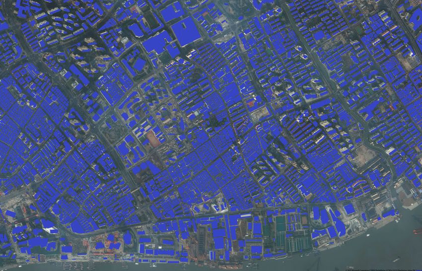
Supplementary Fig. 6 Building footprint with satellite imagery (Shanghai). Satellite image
copyright Microsoft (Bing Map).
30You can also read