Spatial and temporal variations of air pollution over 41 cities of India during the COVID 19 lockdown period - Nature
←
→
Page content transcription
If your browser does not render page correctly, please read the page content below
www.nature.com/scientificreports
OPEN Spatial and temporal variations
of air pollution over 41 cities
of India during the COVID‑19
lockdown period
Krishna Prasad Vadrevu1*, Aditya Eaturu2, Sumalika Biswas3, Kristofer Lasko4, Saroj Sahu5,
J. K. Garg6 & Chris Justice7
In this study, we characterize the impacts of COVID-19 on air pollution using NO2 and Aerosol Optical
Depth (AOD) from TROPOMI and MODIS satellite datasets for 41 cities in India. Specifically, our results
suggested a 13% NO2 reduction during the lockdown (March 25–May 3rd, 2020) compared to the pre-
lockdown (January 1st–March 24th, 2020) period. Also, a 19% reduction in NO2 was observed during
the 2020-lockdown as compared to the same period during 2019. The top cities where NO2 reduction
occurred were New Delhi (61.74%), Delhi (60.37%), Bangalore (48.25%), Ahmedabad (46.20%),
Nagpur (46.13%), Gandhinagar (45.64) and Mumbai (43.08%) with less reduction in coastal cities. The
temporal analysis revealed a progressive decrease in NO2 for all seven cities during the 2020 lockdown
period. Results also suggested spatial differences, i.e., as the distance from the city center increased,
the NO2 levels decreased exponentially. In contrast, to the decreased NO2 observed for most of the
cities, we observed an increase in NO2 for cities in Northeast India during the 2020 lockdown period
and attribute it to vegetation fires. The NO2 temporal patterns matched the AOD signal; however, the
correlations were poor. Overall, our results highlight COVID-19 impacts on NO2, and the results can
inform pollution mitigation efforts across different cities of India.
In early 2020, the COVID-19 virus started to spread rapidly across the globe into most countries, including
India where the first case reported on January 30th, 2020. The latest information pertaining to the number of
COVID-19 active cases, cured discharged statistics, and other public health-related information is reported on
the Ministry of Health and Family Welfare, Government of India website (https://www.mohfw.gov.in/). As per
the website on May 20th, 2020, the total number of active cases was reported to be 61,149, with 42,297 cured/
discharged and 3,303 deaths. Of the different states, Maharashtra had the highest number of cases, followed by
Gujarat, Delhi, Tamil Nadu. There are currently no confirmed cases reported in Arunachal Pradesh, Sikkim,
Nagaland, Mizoram, etc.
India lockdown period. With the COVID-19 outbreak spreading in more than twelve states, by the third
week of March 2020, the Government of India invoked the Epidemic Diseases Act, 1897 and government, edu-
cational, commercial establishments were shut down, including the suspension of all tourist visas. Initially, on
March 22nd, 2020, the Prime Minister announced a 14-h public curfew for the country, with lockdowns in
seventy-five districts where COVID-19 cases had occurred. Shortly thereafter, on March 24th, a nationwide
Phase-1 lockdown was announced for 21 days (March25–April 14th, 2020) affecting the entire 1.3 billion popu-
lation of India.
Further, on April 14th 2020, the Prime Minister implemented Phase-2 which extended the ongoing nation-
wide lockdown until May 3rd. During the lockdown, all commercial and non-commercial activities came to a
1
NASA Marshall Space Flight Center, Huntsville, AL 35811, USA. 2University of Alabama in Huntsville, Huntsville,
AL, USA. 3Smithsonian Conservation Biology Institute, Front Royal, VA, USA. 4US Army Corps of Engineers,
Alexandria, VA, USA. 5Utkal University, Bhubaneswar, Odisha, India. 6Tata Energy Research Institute (TERI)
School of Advanced Studies, New Delhi, India. 7University of Maryland, College Park, MD, USA. *email:
krishna.p.vadrevu@nasa.gov
Scientific Reports | (2020) 10:16574 | https://doi.org/10.1038/s41598-020-72271-5 1
Vol.:(0123456789)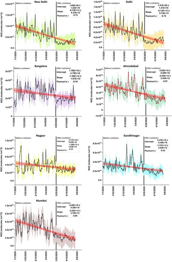
www.nature.com/scientificreports/
halt. For example, all factories, markets, and shops were closed, including any public gathering and places of
worship. People across the country were asked to stay home and practice social distancing if they could not
remain at home. A recent report by the Oxford COVID-19 Government Response Tracker1, based on data from
73 countries reported that India had one of the most stringent measures with respect to “swift action, emergency
policy-making, emergency investment in healthcare, fiscal measures, investment in vaccine research and active
response to the situation, and scored India with a “100” for its strictness”1.
After nearly five weeks of total nationwide lockdown, the Phase-3 of the lockdown was announced from May
4th–May 17th 2020, characterized by partial reopening. The 733 districts in the country were divided into green,
orange, and red zones based on the number of active COVID-19 cases. The green and orange zones were given
a relatively relaxed set of restrictions, whereas the red zones were more restrictive. For example, in a red-zone,
entry and exit was restricted with specific timings to obtain grocery essentials. Also, in the red-zone, e-commerce
players could not deliver non-essentials, and only permitted bicycle, autorickshaws, and taxicabs traffic. Private
establishments were allowed to operate with a 33% staff strength, and movement was not permitted between
7 pm and 7am.
Phase 4 of the nationwide lockdown was announced on May 17th, 2020 and extended until May 31st. As a
part of the fourth phase, the States and Union Territories (UT’s) of India were given the authority to delineate
Red, Green, and Orange Zones as a function of how the COVID-19 situation evolved. The fourth phase insti-
tuted a slow reopening with several relaxations. For example (a) inter-state movement of passenger vehicles was
permitted with mutual consent between states; the intra-state movement of passenger vehicles and buses, to be
determined by States and UTs; (b) essential services were allowed to resume within specified containment zones;
(c) restaurants were permitted to operate kitchens only for home delivery of food, etc. (d) sports complexes and
stadiums were allowed to open, without spectators. Overall, the Government of India has been following stringent
measures to reduce the spread of COVID-19. Of the four different phases, the most restrictive lockdown phase
was from March 25th–May 8th, 2020 (Phase-1 and 2) which is the focus of this study.
Questions addressed
It is well known that air pollution in several regions of the world is due largely to human activities, such as from
fossil fuel combustion from motor vehicles, industries, power plants, etc. With the COVID-19 pandemic, a
reduction in pollution has been reported by several researchers in different regions of the world such as Italy, the
USA and S pain2–5. As a result of the COVID-19 pandemic, during March 25th–May 3rd, 2020 entire India was
lockdown. As a result, there was reduction in pollution in Indian cities t oo6,7. However, the specific amount of
pollution decrease is not well-documented covering multiple cities in India, hence the focus of this study. Some of
the metropolitan cities such as New Delhi, Bangalore, Mumbai in India are renowned for its air pollution. Since,
cities are hotspots of air pollution, we focused on 41 cities based on their population size and analyzed how the
air pollution varied during the lockdown period as compared to the previous year as well as the pre-lockdown
period. We addressed the following questions: (a) How much was NO2 pollution reduced during Phase-1 and 2
of the COVID-19 full country lockdown (March 25-May 3rd, denoted here as 2020-lockdown)? (b) Specifically,
how did NO2 in the 2020-lockdown compare to the same period in 2019, when there was no lockdown (denoted
as 2019-no lockdown)? (c) How did N O2 levels during the 2020-lockdown compare with January–March 24th
2020 (denoted here as 2020-pre-lockdown)? (d) Were the differences in NO2 pollution reduction consistent
across 41 cities? (e) Which cities had the highest and least reduction in NO2? (f) Are there scaling effects in NO2
levels in cities, i.e., based on the spatial distance to the city center? (g) What was the overall reduction in NO2 for
major cities across India and are the differences statistically significant? We addressed these questions using the
remote sensing derived TROPOMI-NO2 datasets and the MODIS Aerosol Optical Depth (AOD) data covering
different cities in India. We focused on satellite-derived N O2 only since the measurement algorithm is relative
matured ones compared to the other gases. Also, adverse health effects of N O2 include acute respiratory illness,
decreased pulmonary function, asthma, lung cancer and cardiopulmonary mortality8; thus, it is important to
address spatial and temporal variations in N O2 useful for pollution management and mitigation purposes.
Cities studied
We selected the 41 cities in India, based on 7 different categories ranked by population (Fig. 1). Rank-1 cities have
the highest population of 5.0 million or greater, and rank-7 cities have less than 50,000 people. A map of the 41
cities selected for the study is shown in Fig. 1. The results of our analysis of the spatial and temporal variation
in the pollution levels are presented for: (a) individual cities; (b) averaged results based on the city’s population
ranking; (c) the top-seven highest polluted cities; (e) cities in northeast India and (f) coastal cities.
Datasets
We used the TROPOspheric Monitoring Instrument (TROPOMI) onboard the Sentinel 5 precursor (S5P), oper-
ated by the European Space Agency (ESA)9 to assess the tropospheric NO2 background levels. Sentinel-5 Precur-
sor (Sentinel-5 P), launched on 13th October 2017, was the first Copernicus mission satellite and can measure
several trace gases such as NO2, ozone, formaldehyde, SO2, methane, carbon monoxide, and aerosols. The resolu-
tion is for all gases with 3.5 × 7 km2, except for CO and C H4, which is 7 × 7 km2. The TROPOMI instrument con-
tains three spectrometers that cover the ultraviolet-near infrared region with two spectral bands at 270–500 nm
and 675–775 nm and one spectrometer that covers the shortwave infrared band. Relatively, TROPOMI has a
higher resolution compared to its predecessor, OMI which has a ground resolution of 13 km × 24 km at nadir.
The TROPOMI N O2 retrieval algorithm utilizes the bands of the ultraviolet-near-infrared spectrometer10. The
retrievals are based on the NO2 DOMINO system which was previously used for OMI s pectra11 with additional
improvements10. The N O2 slant column density is retrieved using the differential optical absorption spectroscopy
Scientific Reports | (2020) 10:16574 | https://doi.org/10.1038/s41598-020-72271-5 2
Vol:.(1234567890)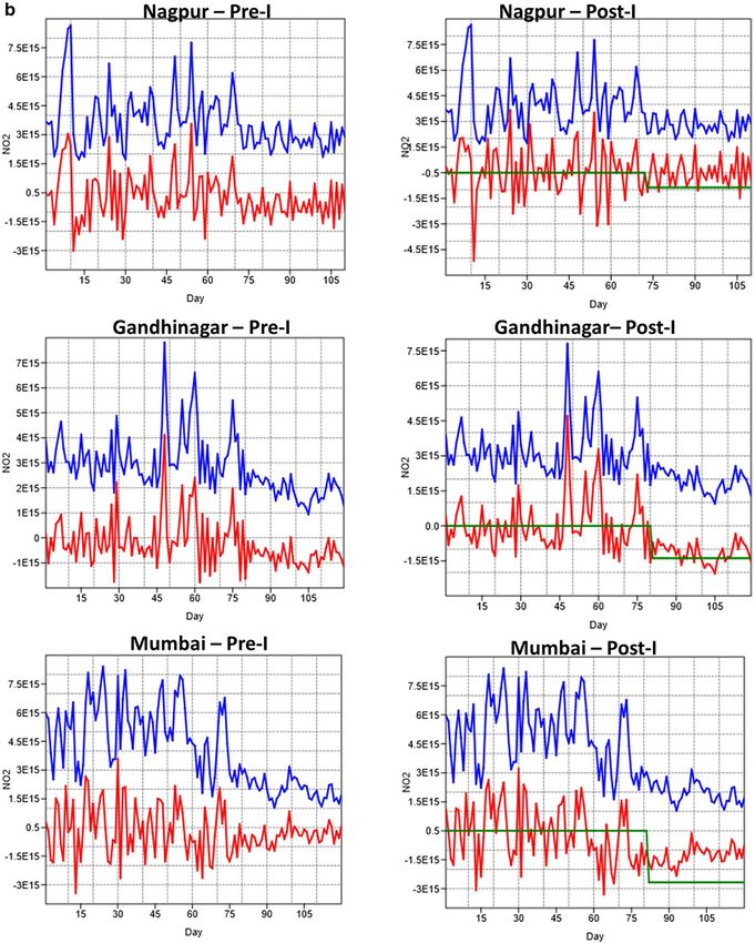
www.nature.com/scientificreports/
Figure 1. Map of India showing location and population in 41 different cities (QGIS software (3.10) QGIS.org
(2020) was used, accessible from https://qgis.org/).
(DOAS) method and separated into stratospheric and tropospheric components using the information from
the data assimilation system and separation based on the altitude dependent air mass factors based on the
lookup table approach. The final product provides the tropospheric vertical column densities, which describes
the vertically integrated number of N O2 molecules per unit area from the surface to tropopause. The data can
be accessed either through the Near-Real-Time (NRTI) stream, the Offline stream (OFFL), or the Reprocessing
(RPRO) stream. NRTI data are available within three hours after data acquisition, whereas OFFL and RPROdata
are available within a few days after acquisition10. In this study, we used the TROPOMI, near-real-time opera-
tional product9 obtained via the Copernicus open data access hub (https://s5phub.copernicus.eu). Independ-
ent validation by the S5P Mission Performance Center (MPC) and S5P validation team concluded that OFFL
level 2 NO2data are in overall agreement with reference measurements collected from global ground-based
networks12–14. In addition to TROPOMI NO2, we also used the MODIS product MCD19A2.006: Terra and Aqua
Multi-angle Implementation of Atmospheric Correction (MAIAC) Land Aerosol Optical Depth (AOD) gridded
Level 2 product, specifically, the blue band (0.17um) 1-km daily data over land14,15 for our study. All processing
was done using the QGIS software (3.10) “QGIS.org (2020). QGIS Geographic Information System. Open Source
Geospatial Foundation Project https://qgis.org/”.
Methods
To generate time series of N O2 columns over 41 different cities, we first selected pixels from an overpass area,
defined by a different buffer radius (30, 45, 60, 75, 90 in km from the city center). We used data for which the
O2 retrieval window is below 40%6.
quality assurance value is higher than 0.5 and the cloud fraction within the N
The averaged tropospheric N O2 column for each city within the buffer radius is calculated as,
Scientific Reports | (2020) 10:16574 | https://doi.org/10.1038/s41598-020-72271-5 3
Vol.:(0123456789)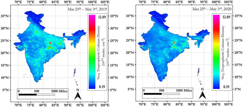
www.nature.com/scientificreports/
kmax
k=1 Dk,d
Ak,d = kmax
k=1 Nk,d
where, Ak,d is the average value of the data for each city during the time period of observations, Dk,d is the aver-
age value of the data for each grid cell ‘k’ within the buffer radius (in km), for each day ‘d’ of the month, over the
time period of the observations and ‘Nk,d ’ being the total number of days of observations for each city within a
specific period, i.e., before or after lockdown. After obtaining the averaged NO2 value for individual cities ( Ak,d )
within a specified buffer distance and time period, we then used the individual values for all the 41 cities to
obtain an average for entire India as,
kmax
(Dk,d,c ∗ Nk,d,c )
Md,c = k=1 kmax
k=1 Nk,d,c
where, ‘ Md,c ’ is the average N
O2 for 41 cities during the period of observations i.e., before and after lockdown,
Dk,d,c is the average NO2 for each city over a period of observations with each grid cell within the city as ‘k’, day
‘d’ and with Nk,d,c being the total number of days of observations for all cities.
Paired t‑test. We used the paired t-test16,17 to compare the mean differences between NO2 pollution lev-
els during different months for the previous (2019) and the current year (2020). The t-test follows a Student’s
t-distribution under the null hypothesis of H0 that the means are equal, H 0: µ1 = µ2 with the alternative hypoth-
esis that Ha: µ1 ≠ µ2. The p-value is used to reject or accept the null hypothesis. The H0 hypothesis was discarded
when the p-value was less than 0.05 (significance level of 5% in this study) and the H a hypothesis is accepted18.
Autoregressive moving average model with intervention. We used the univariate autoregressive
moving-average (ARMA) analysis19,20 with the intervention21,22 to quantify the impacts of COVID-19 on the
pollution levels. Specifically, ARMA models are developed as linear functions of N O2 values with the random
shocks or errors based on the lockdown dates. The main difference between the ARMA model and ARIMA
model is the integral part of the latter, i.e., a measure of how many nonseasonal difference values are needed to
obtain stationarity. Thus, if no differencing is involved, then the model becomes ARMA. In this study, we imple-
mented the ARMA modeling framework in three important steps8 (a) identification of the model; (b) estima-
tion of the coefficients and (c) verification of the model. All these steps are implemented in an iterative process,
resulting in a number of tentative models. First or second-order differencing (nonseasonal and/or seasonal) is
useful for the non-stationary means. The identification of the number of terms to be included in the ARMA
model is based on the analysis of the autocorrelation (ACF) and partial autocorrelation (PACF) functions of
the differenced time series data. The model coefficients were estimated by means of the maximum likelihood
method. Also, the verification of the model is performed through diagnostic checks of residuals through the
normal probability plots and standardized residuals. Finally, Akaike’s Information Criteria (AIC) and Log-like-
lihood criterion were used to establish the model fit.
The intervention analysis helps to determine whether an event affects a timeseries of data, the known source
and timing of intervention due to COVID-19, and the datasets in our case are is 2020-pre lockdown (January
1st–March 24th, 2020) versus 2020 lockdown period (March 25th–May 8th, 2020). The basic ARIMA model is
given as (Eq. 1), when the intervention-free time series Ztfollows the ARIMA (p = autoregressive parameter or
the number of lag observations included in the model, also called the lag-order; d = the number of times the raw
observations are differenced or degree of differencing and q = size of the moving average window) × (P,D,Q)s
(pre-intervention) model with the seasonal period of S, an external shock, mt, has an additive impact. Zt is the
time series before the COVID outbreak and mt is the function indicating the impact of the outbreak.
Yt = mt + Zt
(1 − B)d (1 − B)D �p (B)�p Bs Zt = θ0 + θq (B)�Q Bs at (1)
In the above equation, Yt includes the intervention, �p (B) is a non-seasonal AR polynomial, �p (Bs ) is a sea-
sonal AR polynomial, θq (B) is the non-seasonal MA polynomial, �Q (Bs ) is the seasonal MA polynomial, and at
is the white noise WN (0, σ2). As mentioned, we used only ARMA model in our study.
Further, following the Box and Jenkins19, the intervention effect m t (due to COVID-19 in our case) can be
(T) (T)
calculated as either with the pulse function Pt or the step function St .
(T) 0, t �= T
Pt =
1, t = T (2)
(T) 0, t < T
St =
1, t ≥ T (3)
The pulse function is generally used when a certain event happens at time T, and its effect is limited (Eq. 2),
whereas step function is used when the event is continuous after T (Eq. 3). In the above calculation, an indicator
function either a unit step or a unit pulse20 are transformed by an AR(1) process with a parameter delta, and then
scaled by a magnitude which is the coefficient on the transformed indicator function21,22. Thus, the model can
Scientific Reports | (2020) 10:16574 | https://doi.org/10.1038/s41598-020-72271-5 4
Vol:.(1234567890)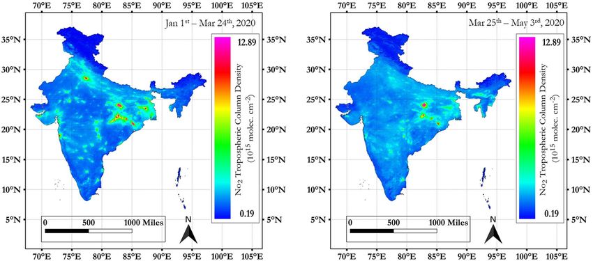
www.nature.com/scientificreports/
Figure 2. Spatial variations in mean tropospheric N
O2 during 2019 (March 25th–May 3rd) non lock down
versus 2020 (March 25th–May 3rd) COVID lock down period, India (QGIS software (3.10) QGIS.org (2020)
was used, accessible from https://qgis.org/).
represent changes that are abrupt and permanent (step function with delta = 0, or pulse with delta = 1), abrupt
and non-permanent (pulse with delta < 1), or gradual and permanent (step with delta < 0). The algorithm is
based on the ARMA transformation and linear regression to find the magnitude. We tried a step function, as
our data fits such a context (with COVID-19 impacts on NO2 reduction, which continued from March 25th to
agnitude22 with the ARMA intervention a nalysis23.
April 3rd) to arrive at the smallest standard error on the m
The ARMA results are reported for before and after the intervention for seven dominant cities where NO2 pol-
lution was most evident.
Results
NO2 variations for all 41 cities. Spatial variations in mean tropospheric NO2 during 2019 (March 25th–
May 3rd) non-lockdown versus 2020 (March 25th–May 3rd) COVID lockdown period for India is shown in
Fig. 2 and 2020 (January 1st–March 24th) pre-lock down versus 2020 COVID lockdown period, is shown in
Fig. 3. Also, details for each city for the mean tropospheric NO2 variations for 2020 pre and post-lockdown
periods is provided in Supplementary Materials.
To infer the data quality, we used the violin plots (Fig. 4) that combine the basic summary statistics of a box
plot with a kernel density plot. In the violin plots, the thick black bar in the center represents the interquartile
range, the central white dot represents the median value, and the whiskers show a 1.5 × interquartile range
(IQR) in the rest of the data. On each side of the black line is a kernel density estimation to show the shape of
the data distribution. The wider sections of the violin plot represent a higher density of observations, and the
skinnier sections represent lower density. Thus, for example, for the 2020 lockdown data, the violin is thicker in
the center, suggesting that most of the values had consistently higher frequency around the median. In contrast,
2019-January and 2019-February data had relatively higher tapering ends with elongated distribution of the data
compared to the other plot. Further, a clear decrease in the median N O2 value can be seen, i.e., in general, the
NO2 pollution during the 2020 pre-lockdown period was considerably less for all 41 cities compared to 2019.
The IQR is a measure of variability; thus, for 2019-January data, it is higher, suggesting the N
O2 values are more
spread out from the median value compared to the 2020 lockdown period (Fig. 4). While we don’t intend to
quantify drivers of these variations, there are many complex interacting factors like transportation, industry,
biomass burning, etc., that might have affected these values.
The paired t-test was quite useful to infer the statistical significance between the two datasets for different
months of 2019-no lockdown versus 2020 lockdown. For example, the results from January-2019 versus Janu-
ary-2020 mean tropospheric N O2 for all 41 cities suggested an overall reduction by 11%, and the results from
the paired t-test were statistically different (January 2019, M = 3.05e+15, SD = 2.53e+15) versus (January 2020,
M = 2.57e+15, SD = 1.90e+15); t(40) = (4.21), p = 0.0001. Since the p-value is less than 0.05 (significant level of
95%), we rejected the null hypothesis and accepted the alternate hypothesis that mean differences between the
two independent data exists, suggesting a decrease in pollution.
The results from February-2019 NO2 versus February-2020 NO2 suggested an overall reduction of 8%, and
the results from the paired t-test were statistically different (February 2019, M = 2.75e+15, SD = 2.13e+15) versus
(February 2020, M = 2.43e+15, SD = 1.63e+15); t(40) = (2.992), p = 0.0047. Since the p-value is less than 0.05
(significant level of 95%), we rejected the null hypothesis and accepted the alternate hypothesis that mean dif-
ferences between the two independent data exists, suggesting a decrease in pollution.
Scientific Reports | (2020) 10:16574 | https://doi.org/10.1038/s41598-020-72271-5 5
Vol.:(0123456789)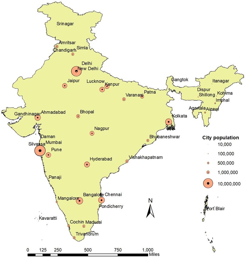
www.nature.com/scientificreports/
Figure 3. Spatial variations in mean tropospheric N
O2 during 2020 (January 1st–March 24th) non lock down
versus 2020 (March 25th–May 3rd) COVID lock down period, India (QGIS software (3.10) QGIS.org (2020)
was used, accessible from https://qgis.org/).
Figure 4. Violin plot depicting N
O2 variations for 41 cities in India. A clear reduction in N
O2 can be seen
during the 2020 lock down period (March 25th–May 3rd, 2020).
Similarly, analysis for March-2019 NO2 versus March 24th 2020 (pre lockdown) NO2 suggested an overall
O2 reduction of 12% and similar to January and February, the results were statistically different (March-2019,
N
M = 2.55e+15, SD = 1.97e+14) versus (March-2020, M = 2.28e+15, SD = 2.0e+14); t(40) = (4.940), p = 0.000. Since
the p-value is less than 0.05 (significant level of 95%), we rejected the null hypothesis and accepted the alternate
hypothesis that mean differences between the two independent data exists, suggesting a decrease in pollution.
Analysis of data between March 25th to May 2019 (no-lockdown period) versus March 25th to May 3rd 2020
(COVID lockdown period) suggested an overall NO2 reduction of 19% and the results are statistically differ-
ent (2019 no lockdown, M = 2.45e+15, SD = 1.38e+15) versus (2020 lockdown, M = 1.74e+15, SD = 5.74e+14);
t(40) = (4.393)p = 0.0001. Since the p-value is less than 0.05, we rejected the null hypothesis and accepted the
alternate hypothesis that mean differences between the two independent data exists. In summary, these results
clearly suggest a statistically significant reduction in NO2 pollution during the 2020 for different months and
the lockdown period.
Scientific Reports | (2020) 10:16574 | https://doi.org/10.1038/s41598-020-72271-5 6
Vol:.(1234567890)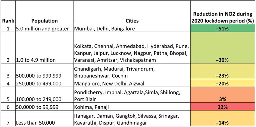
www.nature.com/scientificreports/
Figure 5. Top seven cities in India with NO2 reduction during the lockdown period (March 25th–May 3rd,
2020).
Figure 6. Reduction in tropospheric NO2 levels for top seven cities, India with varying buffer distance from
the city center during COVID lockdown period (March 25th–May 3rd). As the distance from the city center
increased, NO2 levels decreased for all seven cities.
Top seven cities with highest NO2 pollution reduction. The top-seven cities with the highest NO2
pollution reduction based on the data from 2019 no-lockdown versus 2020 COVID lockdown period at 30 km
radius from the center were New Delhi (61.74%), Delhi (60.37%), Bangalore (48.25%), Ahmedabad (46.20%),
etc. (Fig. 5). The mean reduction of N O2 in these seven cities during the 2020 lockdown period is 50.27%. Fur-
ther, we also calculated the NO2 variations during the 2020-pre lockdown versus 2020 lockdown and found an
almost 50.47% reduction during the 2020 lockdown period.
We also did a buffer analysis to infer the spatial scaling effects on the reduction in NO2 for different cities.
From the city center based on the latitude and longitude, the mean tropospheric N O2 were analyzed at varying
Scientific Reports | (2020) 10:16574 | https://doi.org/10.1038/s41598-020-72271-5 7
Vol.:(0123456789)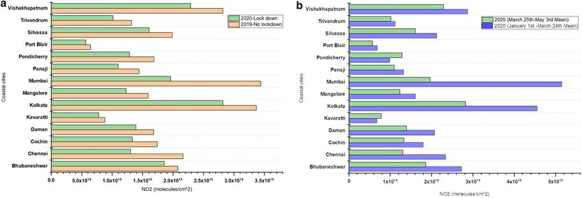
www.nature.com/scientificreports/
Figure 7. Time series N O2 plots for top seven cities, India from January 1 to May 3rd, 2020 COVID. The N O2
data is represented as black lines with dots and the standard errors in different shaded colors along with the
red regression line and 95% confidence bands in orange. The COVID lockdown period start date (March 3rd,
2020) is shown as vertical black line, after which a clear decline in N
O2 pollution can be seen for all cities. Trend
characteristics of slope, intercept and Pearson’s R for the entire range of data are also given for each plot.
Scientific Reports | (2020) 10:16574 | https://doi.org/10.1038/s41598-020-72271-5 8
Vol:.(1234567890)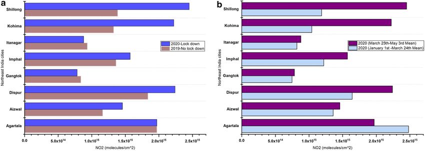
www.nature.com/scientificreports/
Figure 8. Time series ARMA analysis for the seven cities before (Pre-I) and after (Post-I) COVID intervention.
The blue line represents the NO2 data, the redline represents the residuals and the green line represents the
intervention. A clear decrease in N
O2 levels can be seen after day 75 (March 25th, 2020) due to COVID-19.
Scientific Reports | (2020) 10:16574 | https://doi.org/10.1038/s41598-020-72271-5 9
Vol.:(0123456789)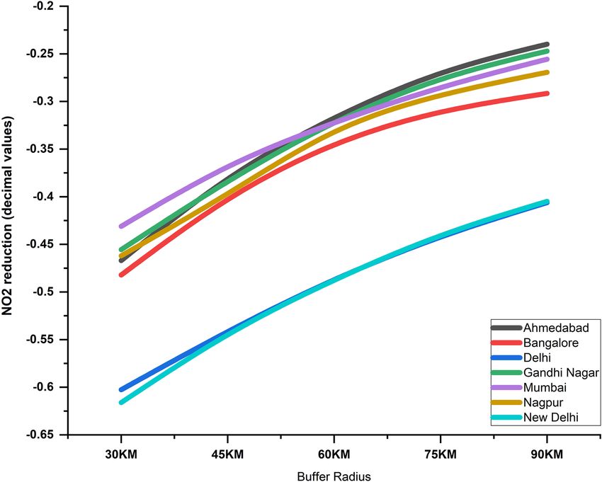
www.nature.com/scientificreports/
Figure 8. (continued)
buffer distances, i.e., 30 km radius, 45, 60, 75, 90 km. Results obtained for N
O2 reduction (in %) for different cities
during the 2020 lockdown period are shown in Fig. 6. Of the different cities, New Delhi and Delhi had the most
NO2 reduction (61.6% and 60.2%), followed by Bangalore (48.2%), Ahmedabad (46.70%), Nagpur (46.20%),
Gandhi Nagar (45.5%) and Mumbai (43.1%) respectively. Further, for all the cities, as the distance from the city
center increased, the NO2 pollution decreased exponentially. Further, of all cities, the highest decrease was noted
for Ahmedabad, followed by Gandhi Nagar, Mumbai, etc. (Fig. 6). We attribute the differences to land cover
variations within the city including local meteorology impacting pollution in these cities.
Time series analysis. The time series plots for 2020 data from January 1st–May 3rd, 2020, for all the seven cities
are shown in Fig. 7. In the figures, data are represented as black lines with the standard errors in the shaded area
along with the regression line in red color and 95% confidence bands in orange. In addition, trend characteristics
of the slope, intercept, and Pearson’s R is also given for each plot. Thus, for example, both New Delhi and Delhi
showed the highest Pearson’s R of − 0.72, followed by Mumbai (− 0.68), Ahmedabad (− 0.61), etc., and least for
Nagpur (r = − 0.32). The slope was larger for New Delhi, followed by Delhi, Mumbai, Ahmedabad, etc., and least
for Bangalore (Fig. 7).
The ARMA modeling was based on the before COVID (pre-intervention) from January 1, 2020–March 24th,
2020 versus during COVID (post-intervention) from March 25th–May 3rd, 2020. Dividing the entire time series
data into two sets helped us to assess the magnitude of differences in NO2 pollution separately. The time series
plots for the seven cities before and during COVID intervention is shown in Fig. 8a,b. In the figures, the blue
line represents the data, the red line represents the residuals, and the green line represents the intervention. The
various AR models fitted for different cities before and after COVID-19 are shown in Tables 1 and 2. An AR(1)
Scientific Reports | (2020) 10:16574 | https://doi.org/10.1038/s41598-020-72271-5 10
Vol:.(1234567890)www.nature.com/scientificreports/
Model
arameters New Delhi Delhi Bangalore Ahmedabad Nagpur Gandhinagar Mumbai
AR (coefficients) 1 (− 0.99) 1 (− 0.999) 1 (− 1) 1 (− 0.776) 1 (− 1) 2 (− 1.37; 0.373) 2 (− 1.50; 0.508)
MA (coeffi- 2 (− 0.664; 2 (− 0.776; 2 (− 0.527;
1 (− 0.90) 1 (− 0.88) 1 (− 0.99) 1 (− 0.938)
cients) − 0.332) − 0.2246) − 0.470)
Log likelihood − 2,663 − 2,695 − 2,711 − 2,916 − 2,614 − 2,883 − 2,945
AIC 5,329 5,393 5,428 5,838 5,234 5,772 5,896
Magnitude − 3.73E15 − 2.19E15 − 8.27E14 − 1.8E15 − 1.26E15 − 1.322E15 − 1.732E15
Standard error 1.67E15 1.716E15 − 2.872E14 3.76E14 5.96E14 4.872E14 1.38E15
Table 1. ARMA model parameters before COVID-19 intervention.
Model parameters New Delhi Delhi Bangalore Ahmedabad Nagpur Gandhinagar Mumbai
3 (− 0.911, 0.063;
AR (coefficients) 1 (− 1) 1 (− 1) 1 (− 0.99) 1 (− 0.918) 1 (− 1) 1 (− 0.99)
− 0.152)
MA (coefficients) 1 (− 0.998) 1 (0.999) 1 (0.637) 1 (− 0.996) 0 1 (− 0.998) 1 (− 0.595; − 0.370)
Log likelihood − 1,442 − 1,366 − 1,395 − 1,360 − 1,386 − 1,392 − 1,423
AIC 2,888 2,735 2,793 2,727 2,774 2,787 2,851
Magnitude − 4.85E15 − 4.36E15 − 7.18E14 − 1.803E15 − 8.64E14 − 1.38E15 − 2.67E15
Standard error 8.061E14 7.99E14 8.84E14 2.76E14 2.116E15 3.34E14 7.54E14
Table 2. ARMA model parameters after COVID-19 intervention.
autoregressive process is one in which the current value is based on the immediately preceding value, while an
AR(2) process is one in which the current value is based on the previous two values. An AR(0) process is used
for white noise and has no dependence between the terms. Results suggested a clear decline in N O2 pollution
(green line in the plots) due to COVID-19. For all cities, the pre-intervention data, too, showed a reduction in
NO2; however, the reduction was much higher during post-intervention as reflected in the ARMA coefficients.
Thus, in all our AR models, the AR coefficients were negative for both pre-and-post intervention COVID data.
In particular, for the post-intervention COVID dataset, the coefficients were highly negative and are below 1,
suggesting that the NO2 reduction is highly persistent. The size of the moving average window for different cit-
ies varied from 0 to 1 for post-intervention COVID data and 1 to 2 for pre-COVID data. Specific to the model
performance or measure of goodness of fit, either log-likelihood or AIC can be used. We used both the indicators
to assess the consistency in the model performance. The higher the value of Log-likelihood, the better the fit of
model coefficients. Thus, for example, post-intervention COVID data consistently had higher values compared to
pre-intervention COVID datasets. In contrast to the Log-likelihood estimator, the lesser the AIC value, the better
the model performance. Thus, a closer examination of Table (1) AIC values suggests that for most of the post-
intervention COVID data, the AIC values are much lower than the pre-intervention COVID data, suggesting
higher performance. Both the Log-likelihood and AIC criterion suggested relatively higher model performances
for the post-intervention COVID data. Further, for both for the pre-and-post intervention COVID data, both
the Log-likelihood and AIC values showed consistency in the order of model performance for different cities.
For example, for the pre-intervention COVID data, the Log-likelihood values were higher for Nagpur, followed
by New Delhi, Delhi, Bangalore, Gandhinagar and Ahmedabad (Table 2); the AIC followed a similar order with
lower values. For the post-intervention COVID data (Table 2), the Log-likelihood ratio estimator showed higher
values for Ahmedabad, Delhi, Nagpur, Gandhinagar, Bangalore, Mumbai, and New Delhi and AIC followed a
similar order with lower values. The intervention effect can also be assessed in terms of magnitude for both pre-
and post-intervention COVID datasets. For both the pre -and post-intervention datasets, the magnitude was
negative, suggesting a decrease in pollution as time progressed; however, the values were more negative for the
post-intervention COVID data compared to the pre-intervention COVID data. Thus, for the pre-intervention
COVID data, a higher reduction in NO2 pollution can be seen for New Delhi, followed by Delhi, Ahmedabad,
Mumbai, Gandhinagar, Nagpur, and Bangalore. For the post-intervention COVID data, a higher reduction in
NO2 pollution can be seen for New Delhi, Delhi, Mumbai, Ahmedabad, Gandhinagar, Nagpur, and Bangalore.
Further, except for Bangalore, where the N O2 reduction was relatively higher for pre-intervention COVID data,
for all the other cities, the post-intervention COVID N O2 reduction was higher than the pre-intervention COVID
datasets. In summary, the ARMA with intervention analysis helped to assess the data in a much more robust way
for assessing the pre-and-post intervention COVID related N O2 reduction.
NO2–MODIS‑AOD relationships. We also explored whether the MODIS AOD could capture variations
in pollution reduction. Although the spatial patterns in tropospheric NO2 and MODIS AOD matched (Supple-
mentary File), they were poorly correlated. For example, the Pearson correlation coefficient (r) for New Delhi
was (0.128), Delhi (0.11), Bangalore (0.02), Ahmedabad (0.07), Nagpur (0.08), Gandhinagar (0.03) and Mumbai
(0.09). The poor correlations can be attributed to the inherent nature of the data. For example, the MODIS AOD
datasets represent coarse and fine particulate aerosols (including dust) for the entire column of the atmosphere,
Scientific Reports | (2020) 10:16574 | https://doi.org/10.1038/s41598-020-72271-5 11
Vol.:(0123456789)www.nature.com/scientificreports/
Table 3. NO2 reduction (%) aggregated based on population ranks for 41 different cities of India. Except for
rank-5 and 6 cities studied, there was a reduction in NO2 levels during 2020 lockdown period (March 25th to
May 3rd) compared to 2019 similar dates. See Supplementary Material for details on individual cities.
Figure 9. (a). Variations in N
O2 for Northeast India cities in India during 2019 no lock down period (March
25th–May 3rd) and 2020 lock down period (March 25th–May 3rd); (b). Data shown for 2020 no lock down
period (averaged NO2 data from January 1st to March 24th) and 2020 lock down period (March 25th–May 3rd).
whereas the NO2 data represents the data for only the troposphere. Despite these differences, both the datasets
showed overall decreasing mean concentrations during the 2020 lockdown period, and the temporal patterns
matched for the specific dates.
Variations in NO2 based on the population rank. Results from the 2019 no-lockdown period versus
2020 lockdown period for various cities based on the population ranks are shown in Table 3. Various population
rank categories are as follows: Rank-1 (5.0 million and greater); Rank-2 (1.0 to 4.9 million); Rank-3 (500,000–
999,999); Rank-4 (250,000–499,000); Rank-5 (100,000–249,000); Rank-6 (500,00–99,999); Rank-7 (< 50,000).
Thus, for Rank-1 population cities, the mean reduction in NO2 was 51%, Rank-2—30%, etc. In the case of
Rank-5 and Rank-6 cities, there was an increase in pollution of 3% and 22%, respectively. We attribute the dif-
ferences to the geographical location; for example, most of the cities (not all) in these two ranks are coastal with
dominant wind and sea breeze influences, compared to the other cities.
Variations in NO2 in northeast Indian cities. In contrast to other cities, northeast Indian cities had an
almost 24% increase in NO2 levels during the 2020 lockdown period compared to the 2019 no-lockdown period
during similar dates. Also, a comparison of NO2 levels for 2020 pre-lockdown versus post lockdown suggested
an average NO2 increase of 36% during the 2020 lockdown period for the cities in northeast India (Fig. 9a,b).
Our preliminary analysis of VIIRS active fire data suggests that an increase in N
O2 levels may be due to vegeta-
Scientific Reports | (2020) 10:16574 | https://doi.org/10.1038/s41598-020-72271-5 12
Vol:.(1234567890)www.nature.com/scientificreports/
Figure 10. Variations in vegetation fires in Northeast India during 2019 no lockdown and 2020 lockdown
period. A clear increase in vegetation fires can be seen for five different cities during 2020 which resulted in
an increase in N
O2 levels during the COVID lockdown period. The specific dates are shown on the top of the
Figure.
Figure 11. (a). Variations in N
O2 for Coastal cities in India during 2019 no lock down period (March 25th–
May 3rd) and 2020 lock down period (March 25th–May 3rd); (b). Data shown for 2020 no lock down period
(averaged NO2 data from January 1st to March 24th) and 2020 lock down period (March 25th–May 3rd).
tion fires, which increased during the 2020 lockdown period compared to 2019 during non-lockdown periods,
especially in areas around the cities of Imphal, Dispur, Kohima, Shillong and Agartala (Fig. 10). A detailed
analysis of N
O2 increase in relation to vegetation fires using daily datasets is ongoing.
Variations in NO2 in coastal cities. Coastal cities had almost 22% N O2 reduction during the 2020 lock-
down period compared to the 2019 no-lockdown period with the highest in Mumbai and Kolkata (Fig. 11a).
Also, a comparison of NO2 levels for 2020 pre-lockdown versus post lockdown suggested an average NO2 reduc-
tion of 30% during the 2020 lockdown period with the highest reduction in Mumbai with a 43.08% reduction
(Figs. 5 and 11b). However, the overall NO2 reduction during the 2020 lockdown period is relatively lower for
the coastal cities compared to the top six non-coastal cities of New Delhi (61.74%), Delhi (60.37%), Bangalore
(48.25%), Ahmedabad (46.20%), Gandhinagar (45.64%), and Nagpur (46.13%).
Ground‑based measurements. We obtained the ground-based NO2 measurement data (µg/m3) for fif-
teen different cities of the total 41 cities of our current focus from the Central Pollution Control Board (CPCB)24,
India. Additional data for the other cities that matched our currently studied cities including spatial and tempo-
ral data from the CPCB were not available. The mean monthly N O2 values during the April lockdown period for
different cities from the ground stations are as follows: Ahmedabad (16.24), Aizawl (0.532), Bangalore (7.934),
Bhopal (11.06), Chandigarh (12.63), Chennai (4.53), Delhi (24.17), Gandhinagar (2.506), Hyderabad (23.54),
Scientific Reports | (2020) 10:16574 | https://doi.org/10.1038/s41598-020-72271-5 13
Vol.:(0123456789)www.nature.com/scientificreports/
Jaipur (12.34), Kanpur (20.78), Kolkata (15.61), Lucknow (19.93), Mumbai (4.43), Nagpur (19.42), Varanasi
(31.68). Further, a comparison of the March 2020 values for these cities suggested an 18% reduction due to
COVID-19 lockdown. These results also match closely with the reduction in NO2 reported for some of the cit-
ies using ground- based measurements6,7. Also, correlating the TROPOMI tropospheric NO2 data for the April
lockdown period suggested a Pearson (r) of 0.33. The poor correlation can be attributed to the satellite data reso-
lution aspects (3.5 × 7 km2), compared to the ground station data footprint which might be much smaller than
the satellite footprint. In addition, we infer that more ground station data at both spatial and temporal scales is
required to validate the satellite data.
Discussion and conclusion
An overview of the results suggests significant differences and patterns in NO2 and AOD which are briefly
highlighted. India has four climatological s easons25, Winter (December–February), Summer or Pre-monsoon
(March–May), Monsoon or rainy season (June to September) and Post-monsoon or autumn season (Octo-
ber–November). Thus, the 2020 lockdown period mostly occurred during the Summer or pre-monsoon season.
In general, most of the cities in the northern part of India see elevated pollution during the post-monsoon
season due to the combined effect of anthropogenic and atmospheric factors. For example, in states of Punjab
and Haryana, important sources of pollution include agricultural residue burning, industrial and vehicular emis-
sions, dust storms, burning of solid fuels for heating, etc., which cause elevated pollution levels not only in these
states but also the neighboring capital city, New D elhi26. In addition, during the post-monsoon season, due to
the temperature inversion, there is less dispersion of pollutants resulting in smog events. In contrast, during the
summer, the dispersion of pollutants is relatively higher compared to the post-monsoon season; the warmer air
is lighter and rises upwards more easily carrying the pollutants away from the land surface and mixes the pol-
lutants with the clear air in the upper layers of the atmosphere27,28, resulting in lesser concentrations. In addition
to the summer effect, due to the COVID-19 lockdown, we found a significant reduction in pollution in major
metropolitan cities. We found several variations, with some cities having more reduction in NO2 than others
in northeast India which experienced an increase in pollution due to the fires during the COVID-19 lockdown
period. More thorough research is needed to understand the fire phenomenon, emissions and meteorology using
the daily datasets. Also, in the coastal areas, the impact of sea and bay breezes on air quality, including air-mass
transportation studies needs to be examined to address the spatial and temporal variations. We also infer the
need to validate satellite measurements with the ground-based measurements. Our results on NO2 reduction
during the COVID-19 lockdown period match with the other studies conducted for some of the cities using the
ground-based measurements and CPCB data from India.
Overall, this study focused on COVID-19 impacts on N O2 pollution. Our results suggested a significant
reduction in NO2 during the lockdown period for most of the cities of India, except those located in Northeast
India. The results from the study include variation in N O2 based on geographical location, population ranks,
distance from the city center, and robust statistical tests to determine the significance of a change in 41 different
cities. Interestingly, we found notably higher vegetation fires during the lockdown period in Northeast Indian
cities which warrant further investigation. The adverse effects of NO2 pollution are well known in the literature.
For example, higher doses of NO2 can cause respiratory ailments8. Also, NO2 and other oxides of nitrogen can
react with water, oxygen and other chemicals to form acid rain which can be harmful to fish and other wildlife.
The acid rain can washout nutrients and minerals from the soil damaging the crops and vegetation including
damage to buildings and structures. Considering these detrimental effects, it is important to arrive at effective
NO2 pollution abatement strategies. Specific to the pollution abatement, the issue of spatial scale is increasingly
being realized. Our results reveal greater variations in terms of N O2 with some cities having the highest reduc-
tion compared to the other based on location and also variations based on the distance to the city center. Thus,
policies to mitigate air pollution can be framed based on the local pollutant variations, needs and priorities.
The spatial NO2 variations highlighted in 41-different cities in our study can serve as a benchmark to address
such variations and can help decision-makers to arrive at efficient air quality management plans involving local
stakeholders. Although a temporary lockdown in emissions due to COVID-19 is a minor reduction in the
overall pollution footprint, the current situation provides some useful insights on how policies like mandatory
lockdown can have a measurable positive impact on the pollution control. As the economy reopens, the emis-
sions will rebound, however, some of the policies such as working remotely could keep emissions under control
post-COVID-19 situation. We also infer a strong need for a political will and social interventions to curb pol-
lution beyond COVID-19 in India.
Received: 27 May 2020; Accepted: 17 August 2020
References
1. OxCGRT. https://www.bsg.ox.ac.uk/research/research-projects/coronavirus-government-response-tracker (2020).
2. Fattorini, D. & Regoli, F. Role of the chronic air pollution levels in the Covid-19 outbreak risk in Italy. Environ. Pollut. 264, 114732
(2020).
3. Bashir, M. et al. Correlation between environmental pollution indicators and COVID-19 pandemic: a brief study in Californian
context. Environ. Res. 187, 109652 (2020).
4. Collivignarelli, M. C. et al. Lockdown for CoViD-2019 in Milan: what are the effects on air quality?. Sci. Total Environ. 732, 139280
(2020).
5. Zambrano-Monserrate, M. A. et al. Indirect effects of COVID-19 on the environment. Sci. Total Environ. 728, 138813 (2020).
6. Devara, P. et al. Influence of air pollution on coronavirus (COVID-19): some evidences from studies at AUH, Gurugram, India.
Sci. Total Environ. https://doi.org/10.2139/ssrn.3588060 (2020).
Scientific Reports | (2020) 10:16574 | https://doi.org/10.1038/s41598-020-72271-5 14
Vol:.(1234567890)www.nature.com/scientificreports/
7. Mahato, S., Pal, S. & Ghosh, K. G. Effect of lockdown amid COVID-19 pandemic on air quality of the megacity Delhi, India. Sci.
Total Environ. 730, 139086 (2020).
8. Pope, C., Mays, N. & Popay, J. Synthesizing Qualitative and Quantitative Health Evidence, a Guide to Methods 330–331 (Open
University Press, Maidenhead, 2007).
9. Veefkind, J. P. et al. TROPOMI on the ESA Sentinel-5 Precursor: a GMES mission for global observations of the atmospheric
composition for climate, air quality and ozone layer applications. Remote Sens. Environ. 120, 70–83 (2012).
10. van Geffen, et al. TROPOMI ATBD of the Total and Tropospheric NO2Data Products. https://www.TROPOMI.eu/documents/
atbd/ (2020).
11. Boersma, K. F. et al. An improved tropospheric NO2 column retrieval algorithm for the ozone monitoring instrument. Atmos.
Meas. Tech. 4(9), 1905 (2011).
12. Eskes, H. J. & Eichmann, K.-U. S5P Mission Performance Centre Nitrogen Dioxide [L2 NO2] https://www.TROPOMI.eu/data-
products/validation (2020).
13. Lambert, J.C., et al. Quarterly Validation Report of the Copernicus Sentinel-5 Precursor Operational Data Products #02: https://
www.TROPOMI.eu/sites/default/files/files/publicS5P-MPC-IASB-ROCVR-02.0.2-20190411_FINAL.pdf (2020).
14. Zhao, X. et al. Assessment of the quality of TROPOMI high-spatial-resolution N O2 data products in the Greater Toronto Area.
Atmos. Meas. Tech. 13(4), 2131–2159 (2020).
15. Lyapustin, A. MODIS Multi-Angle Implementation of Atmospheric Correction (MAIAC) Data User’s Guide. V.2.0. https://lpdaa
c.usgs.gov/documents/110/MCD19_User_Guide_V6.pdf (2018).
16. Freedman, D. A., Pisani, R. & Purves, R. Statistics 93–110 (W. W. Norton & Co Inc, New York, 2007).
17. Kirkwood, B. R. & Sterne, J. A. Essential Medical Statistics 2nd edn, 115–132 (Blackwell, Oxford, 2003).
18. Zar, J. H. Biostatistical Analysis 4th edn, 102–142 (Prentice Hall, Upper Saddle River, 1999).
19. Box, G. E. P. & Jenkins, G. M. Time Series Analysis—Forecasting and Control 57–83 (Holden Day, San Francisco, 1976).
20. Box, G. E. P. & Tiao, G. C. Intervention analysis with applications to economic and environmental problems. J. Am. Stat. Assoc.
70, 70–79 (1975).
21. Tsay, R. S. Time series model specification in the presence of outliers. J. Am. Stat. Assoc. 81(393), 132–141 (1986).
22. Melard, G. A fast algorithm for the exact likelihood of autoregressive-moving average models. J. R. Stat. Soc. Ser. C. 33, 104–114
(1984).
23. Hammer, Ø & Harper, D. A. Paleontological Data Analysis 43–59 (Wiley, Hoboken, 2008).
24. Central Pollution Control Board (CPCB), India. https://www.cpcb.nic.in/ (2020).
25. India Meteorological Department (IMD), India. https://mausam.imd.gov.in/ (2020).
26. Vadrevu, K. P., Lasko, K., Giglio, L. & Justice, C. Vegetation fires, absorbing aerosols and smoke plume characteristics in diverse
biomass burning regions of Asia. Environ. Res. Lett. 10(10), 105003 (2015).
27. Atwater, M. A. Radiative effects of pollutants in the atmospheric boundary layer. J. Atmos. Sci. 28(8), 1367–1373 (1971).
28. Logan, J. A. Nitrogen oxides in the troposphere: global and regional budgets. J. Geophys. Res. Oceans. 88(C15), 10785–10807 (1983).
Acknowledgements
Authors are grateful to the Sentinel-5P and MODIS AOD product developers and for making them freely avail-
able. Authors thank Central Pollution Control Board, New Delhi, India, for providing the ground based N
O2
station data for various cities. The funding support received from the NASA Land Cover/Land Use Change
Program for the South/Southeast Asia Research Initiative is greatly acknowledged.
Author contributions
K.P.V. conceived, analyzed data and wrote the manuscript. AE helped in parts of data processing and cross-
checking. S.B. helped in manuscript formatting and editing. K.L., S.S., G.J.K. and C.J., provided important science
suggestions to strengthen the manuscript, helped in refining and editing.
Competing interests
The authors declare no competing interests.
Additional information
Supplementary information is available for this paper at https://doi.org/10.1038/s41598-020-72271-5.
Correspondence and requests for materials should be addressed to K.P.V.
Reprints and permissions information is available at www.nature.com/reprints.
Publisher’s note Springer Nature remains neutral with regard to jurisdictional claims in published maps and
institutional affiliations.
Open Access This article is licensed under a Creative Commons Attribution 4.0 International
License, which permits use, sharing, adaptation, distribution and reproduction in any medium or
format, as long as you give appropriate credit to the original author(s) and the source, provide a link to the
Creative Commons licence, and indicate if changes were made. The images or other third party material in this
article are included in the article’s Creative Commons licence, unless indicated otherwise in a credit line to the
material. If material is not included in the article’s Creative Commons licence and your intended use is not
permitted by statutory regulation or exceeds the permitted use, you will need to obtain permission directly from
the copyright holder. To view a copy of this licence, visit http://creativecommons.org/licenses/by/4.0/.
© The Author(s) 2020
Scientific Reports | (2020) 10:16574 | https://doi.org/10.1038/s41598-020-72271-5 15
Vol.:(0123456789)You can also read