An Enhanced Ad Event-Prediction Method Based on Feature Engineering
←
→
Page content transcription
If your browser does not render page correctly, please read the page content below
An Enhanced Ad Event-Prediction
                                             Method Based on Feature Engineering
                                                                  Saeid Soheily-Khah and Yiming Wu

                                                                 SKYLADS Research Team, Paris, France
                                                                           {saeid,yiming}@skylads.com

                                        ABSTRACT
                                        In digital advertising, Click-Through Rate (CTR) and Conversion Rate (CVR) are very important
                                        metrics for evaluating ad performance. As a result, ad event prediction systems are vital and
                                        widely used for sponsored search and display advertising as well as Real-Time Bidding (RTB). In
arXiv:1907.01959v1 [cs.LG] 3 Jul 2019

                                        this work, we introduce an enhanced method for ad event prediction (i.e. clicks, conversions) by
                                        proposing a new efficient feature engineering approach. A large real-world event-based dataset of a
                                        running marketing campaign is used to evaluate the efficiency of the proposed prediction algorithm.
                                        The results illustrate the benefits of the proposed ad event prediction approach, which significantly
                                        outperforms the alternative ones.

                                        K EYWORDS
                                        Digital Advertising, Ad Event Prediction, Feature Engineering, Feature Selection, Statistical Test,
                                        Classification

                                        1. Introduction
                                        Ad event prediction is critical to many web applications including recommender systems,
                                        web search, sponsored search, and display advertising [1, 2, 3, 4, 5], and is a hot research
                                        direction in computational advertising [6, 7]. The event prediction is defined to estimate
                                        the ratio of events such as videos, clicks or conversions to impressions of advertisements
                                        that will be displayed. Generally, ads are sold on a ’Pay-Per-Click’ (PPC) basis or even
                                        ’Pay-Per-Acquisition’ (PPA), meaning the company only pays for ad clicks, conversions or
                                        any other pre-defined actions, not ad views. Hence, the Click-Through Rate (CTR) and
                                        the Conversion Rate (CVR) are very important indicators to measure the effectiveness of
                                        advertising display, and to maximize the expected value, one needs to predict the likelihood
                                        that a given ad will be an event, in the accurate way possible. As result, the ad prediction
                                        systems are essential to predict the probabilities of a user doing an action on the ad or
                                        not, and the performance of prediction model has a direct impact on the final advertiser
                                        and publisher revenues and plays a key role in the advertising systems. However, due to
                                        the information of advertising properties, user properties, and context environment, the ad
                                        event prediction is very fancy, challenging and complicated, and is a massive-scale learning
                                        problem.
                                        In the multi-billion dollar online advertising industry, mostly all web applications relied
                                        heavily on the ability of learned models to predict ad event rates accurately, quickly, and
                                        reliably [8, 9, 10]. Even 0.1% of improvement in ad prediction accuracy would yield greater
                                        revenues in the hundreds of millions of dollars. While, with over billions daily active users
                                        and over millions active advertisers, a typical industrial model should provide predictions
                                        on billions of events per day. Hence, one of the main challenges lies in the large design
                                        space to address issues of scale. In the case, for ad event prediction, we need to rely on a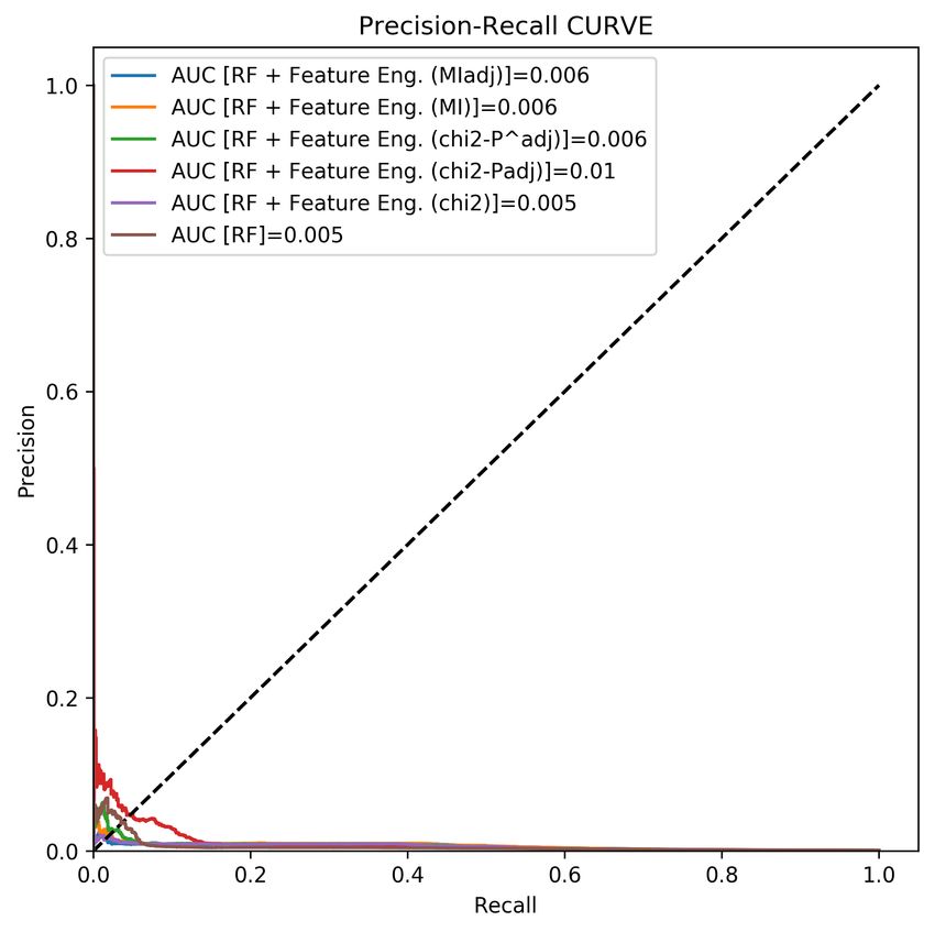
set of well-designed features. However, to capture the underlying data patterns, selecting
and encoding the proper features has also pushed the field.
In this work, we discuss the machine learning methods for ad event prediction and propose a
dedicated feature engineering procedure as well as a new efficient approach to predict more
effectively whether an ad will be an event or not. The novel enhanced algorithm mainly
facilitates feature selection using the proposed statistical techniques, thereby enabling us to
identify, a set of relevant features. The remainder of this paper is organized as follows. In
Section 2, we present briefly the state-of-the-art of a variety of classification techniques which
widely used for ad event prediction applications. Next, we describe machine learning and
data mining methods for feature engineering including feature selection, feature encoding
and feature scaling. In Section 4, we describe the proposed feature engineering strategy
being directly applicable in any event prediction system. Finally, the conducted experiments
and results obtained are discussed in Section 5, and Section 6 concludes the paper. The
main contributions of this research work are as follows:
    - We propose two novel adjusted statistical measures for feature selection.
    - We provide an enhanced framework for ad event-prediction by analyzing the huge
      amount of historical data. The introduced framework includes the pipelines for data
      pre-processing, feature selection , feature encoding, feature scaling, as well as training
      and prediction process.
    - We show through a deep analysis of a very large real-world dataset, that the proposed
      strategy significantly outperform the alternative approaches.
In the remainder of the paper, specially in the experimental study, to simplify, we consider
the events as clicks. Of course, all the design choices, experiments and results can however
be directly extended to any other events such as conversions.

2. State-of-the-art
In the literature, a variety of classification techniques such as logistic regression, support
vector machine, (deep) neural network, nearest neighbor, naive Bayes, decision tree and
random forest have been widely used as machine learning and data mining techniques for
ad event prediction applications.
Logistic regression contains many techniques for modeling and analyzing several features,
when the focus is on the relationship between a dependent feature and one (or more)
independent features. More specifically, the regression analysis is a statistical process which
helps one understand how the typical value of the dependent feature changes when any
one of the independent features is varied, while the other ones are kept fixed. In the
literature, (logistic) regression model have been used by many researchers to solve the ad
event prediction problems for advertising [11, 12, 13, 8].
Gradient boosting is one of the most powerful machine learning algorithms, which produces
a prediction model in the form of hybrid weak models, typically decision trees [14]. The
boosting notion came out of the idea of whether a weak learning model can be modified
to become better. It builds the model in a stage-wise manner like other boosting methods
do, and generalizes them by allowing the optimization of a loss function. Gradient boosting
represents ’gradient descent’ plus ’boosting’, where the learning procedure sequentially fits
novel models to provide a more accurate response estimation. In simple words, the principle
idea behind this method is to construct the novel base-learners to have maximal correlation
with the negative gradient of the loss function, associated with the whole hybrid model.
Gradient boosting technique, practically, is widely used in many prediction applications due
to its easy use, efficiency, accuracy and feasibility [8, 15], as well as the learning applications
[16, 17]. Bayesian classifiers are statistical methods that predict class membership probabilities. They works based on the Bayes’ rules (alternatively Bayes’ law or Bayes’ theorem), where features are assumed to be conditionally independent. Even in spite of assumption of the features dependencies, in practice, they provide satisfying results, they are very easy to implement and fast to evaluate, where they just need a small number of training data to estimate their parameters. However, the main disadvantage is where the Bayesian classifiers make a very strong assumption on the shape of data distribution. In addition, they can not learn interactions between the features, and suffer from zero conditional probability problem (division by zero) [18], where one simple solution would be to add some implicit examples. Furthermore, computing the probabilities for continuous features is not possible by the traditional method of frequency counts. Nevertheless, some studies have found that, with an appropriate pre-processing, Bayesian classifiers can be comparable in performance with other classification algorithms [10, 19, 20, 21]. Neural networks are modeled based on the same analogy to the human brain working, and are a kind of artificial intelligence based methods for ad event prediction problems [22]. Neural networks algorithms benefit from their learning procedures to learn the relationship between inputs and outputs by adjusting the network weights and biases, where the weight refers to strength of connections between two units (i.e. nodes) at different layers. Thus, they are able to predict the accurate class label of the input data. In [23], authors extended Convolutional Neural Network (CNN) for click prediction, however they are biased towards the interactions between neighboring features. Most recently, in [24], authors proposed a factorization machine-supported neural network algorithm, to investigate the potential of training neural networks to predict ad clicks based on multi-field categorical features. However, it is limited by the capability of factorization machines. In general, among deep learning frameworks for predicting ad events, Feed Forward Neural Networks (FFNN) and Probabilistic Neural Network (PNN) are claimed to be the most competitive algorithms. Lastly, random forest [25] is an ensemble learning approach for classification, regression and some other tasks such as estimating the feature importance, which operates by constructing a plenty of decision trees. Particularly, random forest is a combination of decision trees that all together produce predictions and deep intuitions into the data structure. While in standard decision trees, each node is split using the best split among all the features based on the Gini score, while in a random forest, each node is split among a small subset of randomly selected input features to grow the tree at each node. This strategy yields to perform very well in comparison with many other classifiers such as support vector machine, neural network and nearest neighbor. Indeed, it makes them robust against the over-fitting problem as well as an effective tool for classification and prediction [26, 27]. However, applying decision trees and random forests to display advertising, has additional challenges due to having categorical features with very large cardinality and the sparse nature of the data, in the literature, many researchers have used them in predicting ad events [28, 29, 30]. Nevertheless, one of the most vital and necessary steps in any event prediction system is to mine and extract features that are highly correlated with the estimated task. Moreover, many experiment studies are conducted to show that the feature engineering improves the accuracy of ad event prediction systems. The traditional event prediction models mainly depend on the design of features, while the features are artificially selected, encoded and processed. In addition, many successful solutions in both academia and industry rely on manually constructing the synthetic combinatorial features [31, 32]. Because, the data sometimes has a complex mapping relationship, and taking into account the interactions
between the features is vital. In the following, we discuss about state-of-the-art of the
feature engineering approaches, which can be considered as the core problem to online
advertising industry, prior to introduce our proposed approach in feature engineering and
event prediction.

3. Feature engineering
Feature engineering is the fundamental to the application of machine learning, data analysis
and mining as well as mostly all artificial intelligence tasks, and generally, is difficult, costly
and expensive. In any artificial intelligence or machine learning algorithm (e.g. predictive
and classification models), the features in the data are vital, and they dramatically influence
the results we are going to achieve. Therefore, the quantity and quality of the features (and
data) have huge influence on whether the model is good or not. In the following, we discuss
the data pre-processing process and feature engineering in more detail and we present the
most well-used methods in the case.

3.1. Feature selection
Feature selection is the process of finding a subset of useful features and removing irrelevant
features to use in the model construction. It can be used for a) simplification of models
to make them easier to expound, b) reduce training time consumption, c) avoid the curse
of dimensionality and etc. In simple words, feature selection determines the accuracy of a
model and helps remove useless correlation in the data that might diminish the accuracy.
In general, there are three types of feature selection algorithms: filter methods, wrapper
methods and embedded methods.
Embedded approaches learn which features best contribute to model accuracy while it is
being created. It means that some learning algorithms carry out the feature selection as part
of their overall operation, such as random forest and decision tree, where we can evaluate the
importance of features on a classification task. The most common kind of embedded feature
selection approaches are regularization (or penalization) methods, which inset additional
restrictions into the optimization of a predictive algorithm. However, creating such a good
model is challenging due to the computational cost and time of model training.
Wrapper methods consider the selection of a subset of useful features as a search problem,
where different combinations are constructed, evaluated and then compared to other ones.
A predictive model used to assess the combination of features and assign a score based on
the accuracy of the model, where the search process could be stochastic, methodical, or
even heuristic.
Filter feature selection approaches apply a statistical test to assign a goodness scoring value
to each feature. The features are ranked by their goodness score, and then, either selected to
removed from the data or to be kept. These filter selection methods are generally univariate
and consider the feature independently (e.g. chi-square test), or in some cases, with regard
to the dependent feature (e.g. correlation coefficient scores).

3.2. Feature encoding
In machine learning, when we have categorical features, we often have a major issue: how
to deal with categorical features? Practically, one can postpone the problem using a data
mining or machine learning model which handle the categorical features (e.g. k-modes clus-
tering), or deal with the problem (e.g. label encoding, one-hot encoding, binary encoding)
When we use such a learning model with categorical features, we mostly have three types of
models: a) models handling categorical features accurately, b) models handling categorical
features incorrectly, or c) models do not handling the categorical features at all.
Therefore, there is a need to deal with the following problem. Feature encoding points out
to transforming a categorical feature into one or multiple numeric features. One can use
any mathematical or logical approach to convert the categorical feature, and hence, there
are many methods to encode the categorical features, such as: a) numeric encoding, which
assigns an arbitrary number to each feature category, b) one-hot encoding which converts
each categorical feature with m possible values into m binary features, with one and only
one active, c) binary encoding to hash the cardinalities into binary values, d) likelihood
encoding to encode the categorical features with the use of target (i.e. label) feature. From
a mathematical point of view, it means a probability of the target, conditional on each
category value, and e) feature hashing, where a one-way hash function convert data into a
vector (or matrix) of features.

3.3. Feature scaling
Most of the times, the data will contain features highly varying in units, scales and ranges.
Since, most of the machine learning and data mining algorithms use Eucledian distance
between two data points in their computations, this makes a problem. To suppress this
effect, we need to bring all features to the same level of unit, scale or range. This can be
attained by scaling. Therefore, feature scaler is a utility that converts a list of features
into a normalized format suitable for feeding in data mining and learning algorithms. In
practice, there are four common methods to perform feature scaling: a) min-max scaling to
rescale the range of features in [0, 1] or [âĹŠ1, 1], b) mean normalisation to normalize the
values between -1 and 1, c) standardisation, which swaps the values by their Z scores, and
d) unit vector, where feature scaling is done in consideration of the entire feature vector to
be of unit length.
Notice that, generally, in any algorithm that computes distance or assumes normality (such
as nearest-neighbor), we need to scale the features, while feature scaling is not indispensable
in modeling trees, since tree based models are not distance based models and can handle
varying scales and ranges of features. As more examples, we can speed up the gradient
descent method by feature scaling, and hence, it could be favorable in training a neural
network, where doing a features scaling in naive Bayes algorithms may not have much
effect.

4. The design choices
The proposed feature engineering strategy is briefly presented in to the following steps (see
Algorithm 1), where in the reminder of this section, we explain in detail the proposed feature
learning approach for the ad event prediction.
Typically, there are plenty of recorded information, attributes and measures in an executed
marketing campaign. For instance, the logs services enable advertisers to access the raw,
event-level data generated through the online platform in different ways. However, we are
not interested in all of them. Lots of recorded information and data are not useful or
available for us, even they increase the complexity. So, at the first step, we prune the raw
data, before doing any mining task.
Algorithm 1 The proposed feature engineering strategy
 input:  row data
 output: featurescat , featuresnum

  function pre-processing(data)
      remove duplication data
      rebild (or drop) missing (or incomplete) values
      remove (redundant) features with zero (and low) variance
  return data

  function feature selection(data)
      run proposed adjusted chi-squared-test (or adjusted mutual information)
  return featurescat , featuresnum

  function feature encoder(featurescat )
      for each feature i in featurescat
           d value ⇐ number of distinct values for feature i
           if d value>threshold
                do string indexer
                do feature hasher
           else (
values of other features (i.e. variables). In the other hand, the missing data could be not
at random. For instance, people with high salaries generally do not want to reveal their
incomes, or the females generally do not want to reveal their ages. Here the missing value
in ’age’ feature is impacted by the ’gender’ feature. So, we have to be really careful before
removing any missing data. Finally, when we figure out why the data is missing, we can
decide to abandon missing values, or to fill.
As a summary, the most important key benefits of data cleaning in digital marketing are:
– Accurate view of customers, users and audiences; The customers and online users are
the exclusive sources of any analysis and mining task and are central to all business
decision making. However, they are always changing. Their natures, behaviours,
likes and dislikes, their habits, as well as their expectations are in a constant stage
of change. Hence, we need to remain on top of those fluctuations in order to make
smart decisions.
– Improve data integration; Integrating data is vital to gain a complete view of the
customers, users and audiences, and when data is dirty and laden with duplicates
and errors, data integration process will be difficult. In typical, multiple channels
and multiple departments often collect duplicate data for the same user. With data
cleaning, we can omit the useless and duplicate data and integrate it more effectively.
– Increases revenue and productivity
4.2. Feature selection
In feature selection, we rely on the filter methods, and we try to fit two proposed adjusted
statistical measures (i.e. mutual information, chi square test) to the observed data, then
we select the features with the highest statistics. Suppose we have a label variable (i.e. the
event label) and some feature variables that describe the data. We calculate the statistical
test between every feature variable and the label variable and observe the existence of a
relationship between the variable and the label. If the label variable is independent of the
feature variable, we can discard that feature variable. In the following, we present the
proposed statistical measures in detail.
4.2.1. Adjusted chi-squared test
A very popular feature selection method is chi-squared test (χ2 -test). In statistics, the
chi-squared test is applied to test the independence of two events (i.e. features), where two
events X and Y are defined to be independent, if P (XY ) = P (X)P (Y ) or, equivalently,
P (X|Y ) = P (X) and P (Y |X) = P (Y ). The formula for the χ2 is defined as:
X (Oi − Ei )2
χ2df = (1)
Ei
where the subscript df is the degree of freedom, O is the observed value and E the expected
value. The degrees of freedom (df ) is equal to:
df = (r − 1) ∗ (c − 1) (2)
where r is the number of levels for one categorical feature, and c is the number of levels for
the other categorical feature. After taking the following chi-square statistic, we need to find
p-value in the chi-squared table, and decide whether to accept or reject the null hypothesis
(H0 ). The p-value is the probability of observing a sample statistic as extreme as the test
statistic, and the null hypothesis is the case that two categorical features are independent.Generally, small p-values reject the null hypothesis, and very large p-values means that the
null hypothesis should not be rejected. As result, the chi-squared test gives a p-value, which
tells if the test results are significant or not. In order to perform a chi-squared hypothesis
test and get the p-value, one need a) the degree of freedom and b) the level of significance
(α), while the default value is 0.05 (5%).
Like all non-parametric data, the chi-squared test is robust with respect to the distribution
of the data [33]. However, it has difficulty of interpretation when there are large numbers
of categories in the features, and tendency to produce relatively very low p-values, even for
insignificant features. Furthermore, chi-squared test is sensitive to sample size, which is why
several approaches to handle large data have been developed [34]. When the cardinality
is low, it would be a little difficult to get a null hypothesis rejection, whereas a higher
cardinality will be more intended to result a rejection.
In feature selection, we usually calculate the p-values of each feature, then choose those ones
which are smaller than the ’preset’ threshold. Normally, we use α = 0.95, which stands for a
threshold of 5% significance. For those features within this threshold, smaller p-value stands
for better feature. However as mentioned before, higher cardinality will always cause a lower
p-value. This means that the features with higher cardinality, e.g. user identification, or
site URLs, are always having lower p-values, and in turn, to be a better feature, which may
not always be true.
In order to find a more reliable measure other than simply using p-value from chi-squared
test, we proposed a new measure by adding a regularization term on the p-values (pv) of
features, called ’adjusted p-value’ (padj ). The new proposed statistical measure, padj , is
defined as:
χ21−pv,df − χ21−α,df
padj = (3)
χ21−α,df
where α is the level of significance, and df is the degrees of freedom. By using this quantity,
we are penalizing on the features with higher cardinality. Simply to say, we are trying to see
how further by percentage the critical value corresponding to pv, the χ21−pv,df , is crossing
the critical value χ21−α,df , corresponding to a given significance level 1 − α. Note that, the
χ21−α,df will be very big for high cardinality features due to higher degree of freedom, and
it is regarded as a penalization term.
The penalization could also be softer, if we take the logarithm of the critical value χ21−α,df .
In the case, the adjusted p-value with soft penalization, p̂adj , can be formulated as:
χ21−pv,df − χ21−α,df
p̂adj = (4)
log(χ21−α,df )
For the two proposed above measures, higher value stands for better feature.
4.2.2. Adjusted mutual information
Similar to the Chi-square test, the Mutual Information (MI) is a statistic quanitity which
measures how much a categorical variable tells another (mutual dependence between the
two variables). The mutual information has two main properties; a) it can measure any
kind of relationship between random variables, including nonlinear relationships [35], and
b) it is invariant under the transformations in the feature space that are invertible and
differentiable [36]. Therefore, it has been addressed in various kinds of studies with respectto feature selection [37, 38]. It is formulated as:
X P (x, y)
I(X; Y ) = P (x, y) log (5)
x∈X,y∈Y
P (x)P (y)
where I(X; Y ) stands for the ’mutual information’ between two discrete variables X and Y ,
P (x, y) is the joint probability of X and Y , and P (x) and P (y) are the marginal probability
distribution of X and Y, respectively. The MI measure is a non-negative value, and it
is easy to deduce that if X is completely statistically independent from Y , we will get
P (x, y) = P (x)P (y) s.t. x ∈ X, y ∈ Y , which indicates a MI value of 0. The MI is bigger
than 0, if X is not independent from Y .
In simple words, the mutual information measures how much knowing one of the variables
reduces uncertainty about the other one. For example, if X and Y are independent, then
knowing X does not give any information about Y and vice versa, so their mutual informa-
tion is zero.
In the case of feature selection using the label column (Y), if MI is equal to 0, then X is
considered as a ’bad’ single feature, while the bigger MI value suggests more information
provided from the feature X, which should be remained in the classification (predictive)
model. Furthermore, when it comes to optimal feature subset, one can maximize the mutual
information between the subset of selected features xsubset and the label variable Y , as:
ζ = arg max I(xsubset ; Y ) (6)
subset
where |subset| = k, and k is the number of features to select. The quantity ζ is called ’joint
mutual information’, and its maximizing is an N P -hard optimization problem.
However, the mutual information is subject to a Chi-square distribution, that means we can
convert the mutual information to a p-value as a new quantity. This new adjusted measure,
called MIadj , will be more robust than the standard mutual information. Also, we can rule
out those features that is not significant based on the calculated p-value. Normally:
2N ∗ MI ∼ χ2df (7)
where the N stands for the number of data samples, and similar as before, df is degree of
freedom. So simply to say, our proposed new filtering rule (MIadj ) is defined by:
2N ∗ I(X; Y ) − χ0.95,df (X,Y ) > 0 (8)
The bigger MIadj , the better is. Some features will be ruled out if their new adjusted
measures are negative, which indicate the mutual information are not significant comparing
to their degrees of freedom.
4.3. Feature encoding
In the next step, we need to format the data, which can be accepted by the training
model. In practice, we do the training and prediction tasks using Spark in Yarn, because
we have nearly forty million records to analyse on a weekly basis. Specifically, we use the
StringIndexer, which encodes the features by the rank of their occurrence times, for high
cardinality features above a predefined threshold , and one hot encoder for the features
whose unique levels less then the predefined threshold. We also hash the high cardinalityfeatures to ensure that we are formatting the data without loosing too much information.
In a nutshell, in our ad event prediction case, there are some extremely high cardinality
features like user ids, or page urls with millions levels on weekly basis. It’s better to hash
them (rather than one hot encode them) to keep most of the information without facing
the risk of explosion of feature numbers at the meantime.
4.4. Feature scaling
Finally, we do feature scaling according to the max-min scaling method, as a last step in
the feature engineering.
5. Experimental study
In this section, we first describe the dataset used to conduct our experiments, then specify
the validation process, prior to present and discuss the results that we obtained.
5.1. Data description
In this section, to clarify our claim in ad event prediction, we used a large real-world dataset
of a running marketing campaign. The dataset is a private activity report from MediaMath
digital advertising platform, is very huge, and the entire dataset is stored on cloud storage
(i.e. Amazon S3) of Amazon Web Services (AWS). It comprises over 40 millions of recorded
ads data (on weekly basis), each one with more than 80 pieces of information, which can
be categorized in two main group: a) attributes which can be considered as features, and
b) event labels for machine learning and mining tasks.
5.1.1. Attributes (features)
The input features for machine learning algorithms, such as user id, site url, browser, date,
time, location, advertiser, publisher and channel. Notice, that it is highly probable that one
generates new features from the existence ones. For instance, from start-time and stop-time,
we can produce the duration feature, or from date, we can generate the new feature day of
week, which will be more meaningful in the advertising campaign.
5.1.2. Measures (labels)
Measures are the target variables data which acts as labels in machine learning and data
mining algorithms, such as impressions, clicks, conversions, videos, and spend. Note that,
the mentioned measures (i.e. labels) are needed for supervised learning algorithms, while
in non-supervised algorithm one can ignore them.
5.2. Validation process
Here we compare the proposed ad event prediction algorithm with the state-of-the-art and
the well-used feature engineering based event prediction methods. For our comparisons,
we rely on the Accuracy (ACC), recall or True Positive Rate (TPR), precision or Positive
Predictive Value (PPV), F-measure (F1 -SCORE), which is a harmonic mean of precision
and recall, as well as the area under Precision-Recall curve (AUC-PR), which are commonly
used in the literature, to evaluate each method.
Table 1 presents the classical confusion matrix in terms of True Positive (TP), False Positive
(FP), True Negative (TN) and False Negative (FN) values, which are used in the perfor-
mance metrics (P: event, N: normal). Lastly, the above-mentioned comparison measures
are defined as:
TP + TN TP TP
ACC = , TPR = , PPV = (9)
TP + FN + FP + TN TP + FN TP + FPTable 1: Confusion matrix
Predicted class
Positive class Negative class
Positive class TP FN
Actual class
Negative class FP TN
and,
2T P
F1 -SCORE = (10)
2T P + F P + F N
The accuracy measure lies in [0, 100] in percentage, and true positive rate (recall), positive
predictive value (precision), and F-measure lie within a range of [0, 1]. The higher index,
the better the agreement is. In the other side, precision-recall is a useful measure of success
of prediction when the classes are very imbalanced, and the precision-recall curve shows the
trade-off between precision and recall for different threshold. A high area under the curve
represents both high recall and high precision. High scores illustrate that the predictor (or
classifier) is returning accurate results (high precision), as well as returning a majority of
all positive results (high recall). The Precision-Recall (PR) summarizes such a curve as the
weighted mean of precisions achieved at each threshold, with the increase in recall from the
previous threshold used as the weight:
X
PR = (Rn − Rn−1 )Pn (11)
n
where Pn and Rn are the precision and recall at the nth threshold.
For all the methods, the parameters as well as the training and testing sets are formed by
k-fold cross validation in the ratio of 80% and 20% of the data, respectively. For instance,
for the random forest two parameters are tuned: number of trees and minimum sample
leaf size. Finally, the results reported hereinafter are averaged after 10 repetitions of the
corresponding algorithm.
5.3. Experimental results
In the context of event prediction, the accuracy (ACC), recall (TPR), precision (PPV), F-
measure (F1 -SCORE), as well as the area under PR curve (AUC-PR), for the various tested
approaches, are reported in the Table 2. Many papers in the literature have shown that, as
far as heterogeneous multivariate data are concerned, random forest are among the most
efficient methods to be considered [39, 40]. Hence, we build our proposed event prediction
algorithm on the basis of a Random Forest (RF) classifier. To facilitate the big data analysis
task, we do the data pre-processing, training, and ad event prediction by running spark jobs
on Yarn. Note that, the results in bold correspond to the best assessment values.
Table 2 shows the comparison of performances of a simple classifier versus the case of doing
a feature engineering before running the classifier, on a real-world dataset. Notice that,
here, in the feature selection process, we consider only top 20 features. Of course, one can
simply find the best number of features using a k-fold cross validation technique.
As has been pointed out in Table 2, while in feature selection using the standard statistical
approach (i.e. χ2 and MI), the random forest classifier can not provide any good results for
recall (TPR), precision (PPV) and F1 -SCORE, using the proposed statistical metrics (i.e.
χ2 -padj and MIadj ), we generally outperform the results. Also, it is plain to see that theTable 2: Comparison of performances based on the different feature engineering methods
ACC TPR PPV F1 -SCORE AUC-PR
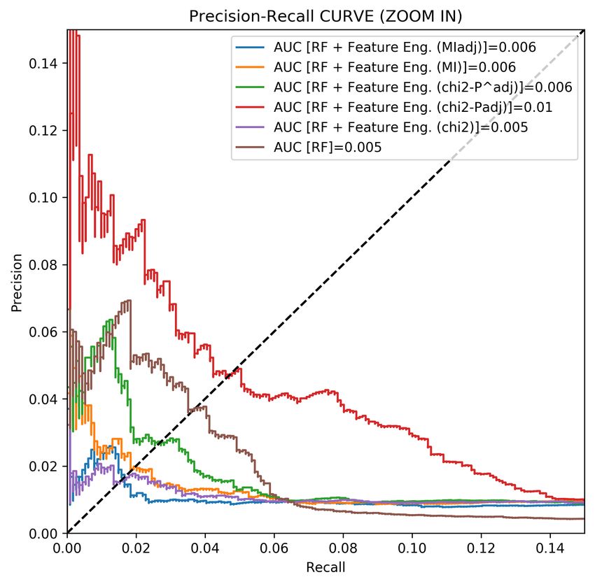
RF 99.61 0.050 0.013 0.022 0.005
RF + Feature Eng. (χ2 ) 99.92 0.000 0.000 0.000 0.005
RF + Feature Eng. (χ2 -padj ) 99.94 0.051 0.044 0.047 0.010
RF + Feature Eng. (χ2 -p̂adj ) 99.92 0.000 0.000 0.000 0.006
RF + Feature Eng. (MI) 99.92 0.000 0.000 0.000 0.006
RF + Feature Eng. (MIadj ) 99.91 0.008 0.023 0.012 0.006
RF classifier with considering feature selection based on the proposed χ2 -padj has the best
results, and outperforms significantly the precision, recall, F-measure as well as the area
under precision-recall curve. However, for this case, the soft penalized version of χ2 -padj (i.e.
χ2 -p̂adj ) does not provide very good result, but still it is better than the standard χ2 and is
comparable with the standard mutual information metric. Furthermore, as demonstrated,
using the proposed adjusted version of mutual information in feature selection process,
provides better results rather than using the standard mutual information measure.
To verify our claim and consolidate the comparative results, we use a Wilcoxon signed rank
test, which is a non-parametric statistical hypothesis test to effectively determine whether
our proposed adjusted statistic measures are significantly outperform the classifier (using
the alternative quantities) or not. Tables 3 presents the two-sided p-value for the hypothesis
test, while the results in bold indicate the significantly different ones. The p-value is the
probability of observing a test statistic more extreme than the observed value under the
null hypothesis. Notice that, the null hypothesis is strongly rejected when the p-values are
lower than a pre-defined criterion, almost always set to 0.05. It means that the differences
between the two tested classifiers are significant and the uniform hypothesis is accepted
as p-values are greater than 0.05. Based on the p-values, we can justify that using the
proposed adjusted measures in feature selection, the classifier leads to significantly better
results than the others. Note that the difference between the pairs of classifiers results
follows a symmetric distribution around zero and to be more precise, the reported p-values
are computed from all the individual results after some repetitions of the corresponding
algorithm.
Table 3: P-values: Wilcoxon test
RF + Feature Eng.
(χ2 ) (χ2 -padj ) (χ2 -p̂adj ) (MI) (MIadj )
RF 0.034 0.004 0.073 0.073 0.798
RF + Feature Eng. (χ2 ) 0.011 0.157 0.157 0.011
RF + Feature Eng. (χ2 -padj ) 0.011 0.011 0.011
RF + Feature Eng. (χ2 -p̂adj ) 1.000 0.026
RF + Feature Eng. (MI) 0.026
As is evident from Table 3, with regard to the p-values of Wilcoxon test, the RF classifier
with considering feature selection method using the proposed χ2 -padj measure, brings a
significant improvement compared to the other methods. In addition, the proposed MIadj
is almost performing significantly different than the other approaches.
To become closely acquainted with selected features, Table 4 shows the top 20 selected
features using different feature selection models (i.e. statistical test) which we consider in
our experimental study.Table 4: Feature selection: top-k extracted features using different statistical test (rank sorted)
χ2 χ2 -padj χ2 -p̂adj MI MIadj
os id id vintage mm uuid mm uuid publisher id
category id os id contextual data contextual data site id
contextual data fold position page url page url site url
week hour advertiser id user agent site id main page
concept id conn speed id strategy id strategy id supply source id
overlapped b pxl watermark creative id site url exchange id
week hour part browser name site id publisher id category id
site id browser language zip code id creative id creative id
norm rr week hour ip address user agent channel type
page url width site url main page concept id
strategy id cross device flag overlapped b pxl zip code id campaign id
app id browser version aib recencies concept id browser name
creative id week hour part main page campaign id browser version
browser version device id city code id city code id model name
zip code id app id concept id supply source id homebiz type id
form factor city campaign id exchange id os id
supply source id week part hour part channel type category id os name
prebid viewability category id homebiz type id model name brand name
brand name norm rr os id norm rr form factor
exchange id dma id form factor channel type norm rr
Note that, in the term of time consumption, all the proposed adjusted statistical test (i.e.
χ2 -padj , χ2 -p̂adj , MIadj ), have more or less the same time complexity with the standard ones
(i.e. χ2 , MI), without any significant difference.
Lastly, to have a closer look at the ability of the proposed statistical quantities, the Figure 1
shows the comparison of the area under PR curve for different feature engineering methods
on the basis of a random forest classifier. Note that, we consider the area under PR curve,
since it is more reliable rather than ROC curve, because of the unbalanced nature of data.
The higher values are the better performance.
Figure 1: Comparison of AUC-PR curve based of different feature engineering methods6. Conclusion
This research work introduces an enhanced ad event prediction framework which has been
applied on big data. In this framework, we propose two statistical approaches which can
be used for feature selection: i) the adjusted Chi-squared test and ii) the adjusted mutual
information. Then, by ranking the statistical measures we select the best features. Also,
in feature encoding before training the model, we used a practical while reliable pipeline
to encode very large (categorical) data. The efficiency of the proposed event prediction
framework is analyzed on a large real-world dataset from a running campaign. The results
illustrate the benefits of the proposed adjusted Chi-squared test (and the adjusted mutual
information), which outperforms the others with respect to different metrics, i.e. accuracy,
precision, recall, F-measure and the area under precision-recall curve. Lastly, a Wilcoxon
signed-rank test is used to determine that the proposed approach is significantly better than
the other methods described in the paper. While, in this research work, we focus on the
single features, the idea of combined features can be a proper proposition to gain better
result. Hence, investigate the combination of some features to generate more useful features,
to further increase the prediction performance of the imbalanced case, which is typical in
the context of digital advertising, can be an interesting suggestion for future works.
7. References
[1] H. Cheng and E. Cantú-Paz, “Personalized click prediction in sponsored search,” in Proceed-
ings of the Third ACM International Conference on Web Search and Data Mining, WSDM
’10, (New York, NY, USA), pp. 351–360, ACM, 2010.
[2] Y. Zhang, H. Dai, C. Xu, J. Feng, T. Wang, J. Bian, B. Wang, and T.-Y. Liu, “Sequential
click prediction for sponsored search with recurrent neural networks,” in Proceedings of the
Twenty-Eighth AAAI Conference on Artificial Intelligence, pp. 1369–1375, AAAI Press, 2014.
[3] O. Chapelle, E. Manavoglu, and R. Rosales, “Simple and scalable response prediction for
display advertising,” ACM Trans. Intell. Syst. Technol., vol. 5, pp. 61:1–61:34, Dec. 2014.
[4] A. Borisov, I. Markov, M. de Rijke, and P. Serdyukov, “A neural click model for web search,”
in Proceedings of the 25th International Conference on World Wide Web, pp. 531–541, 2016.
[5] H.-T. Cheng, L. Koc, J. Harmsen, T. Shaked, T. Chandra, H. Aradhye, G. Anderson, G. Cor-
rado, W. Chai, M. Ispir, R. Anil, Z. Haque, L. Hong, V. Jain, X. Liu, and H. Shah, “Wide &
deep learning for recommender systems,” in Proceedings of the 1st Workshop on Deep Learning
for Recommender Systems, DLRS 2016, (New York, NY, USA), pp. 7–10, ACM, 2016.
[6] C. Li, Y. Lu, Q. Mei, D. Wang, and S. Pandey, “Click-through prediction for advertising
in twitter timeline,” in Proceedings of the 21th ACM SIGKDD International Conference on
Knowledge Discovery and Data Mining, KDD ’15, pp. 1959–1968, ACM, 2015.
[7] J. Chen, B. Sun, H. Li, H. Lu, and X.-S. Hua, “Deep ctr prediction in display advertising,” in
Proceedings of the 24th ACM International Conference on Multimedia, MM ’16, (New York,
NY, USA), pp. 811–820, ACM, 2016.
[8] M. Richardson, E. Dominowska, and R. Ragno, “Predicting clicks: Estimating the click-
through rate for new ads,” in Proceedings of the 16th International Conference on World
Wide Web, WWW ’07, (New York, NY, USA), pp. 521–530, ACM, 2007.
[9] D. Agarwal, B. C. Chen, and P. Elango, “Spatio-temporal models for estimating click-through
rate,” in WWW ’09: Proceedings of the 18th international conference on World wide web, (New
York, NY, USA), pp. 21–30, ACM, 2009.
[10] T. Graepel, J. Q. n. Candela, T. Borchert, and R. Herbrich, “Web-scale bayesian click-
through rate prediction for sponsored search advertising in microsoft’s bing search engine,”
in Proceedings of the 27th International Conference on International Conference on Machine
Learning, ICML’10, (USA), pp. 13–20, Omnipress, 2010.[11] O. Chapelle, “Modeling delayed feedback in display advertising,” in Proceedings of the 20th
ACM SIGKDD International Conference on Knowledge Discovery and Data Mining, KDD
’14, (New York, NY, USA), pp. 1097–1105, ACM, 2014.
[12] M. J. Effendi and S. A. Ali, “Click through rate prediction for contextual advertisment using
linear regression,” CoRR, vol. abs/1701.08744, 2017.
[13] H. B. McMahan, G. Holt, D. Sculley, M. Young, D. Ebner, J. Grady, L. Nie, T. Phillips,
E. Davydov, D. Golovin, S. Chikkerur, D. Liu, M. Wattenberg, A. M. Hrafnkelsson, T. Boulos,
and J. Kubica, “Ad click prediction: a view from the trenches,” in Proceedings of the 19th
ACM SIGKDD International Conference on Knowledge Discovery and Data Mining (KDD),
2013.
[14] J. H. Friedman, “Stochastic gradient boosting,” Comput. Stat. Data Anal., vol. 38, pp. 367–
378, Feb. 2002.
[15] I. Trofimov, A. Kornetova, and V. Topinskiy, “Using boosted trees for click-through rate
prediction for sponsored search,” in Proceedings of the Sixth International Workshop on Data
Mining for Online Advertising and Internet Economy, ADKDD ’12, (New York, NY, USA),
pp. 2:1–2:6, ACM, 2012.
[16] C. J. C. Burges, “From RankNet to LambdaRank to LambdaMART: An overview,” tech.
rep., Microsoft Research, 2010.
[17] K. S. Dave and V. Varma, “Learning the click-through rate for rare/new ads from similar
ads,” in Proceedings of the 33rd International ACM SIGIR Conference on Research and De-
velopment in Information Retrieval, SIGIR ’10, (New York, NY, USA), pp. 897–898, ACM,
2010.
[18] P. Domingos and M. Pazzani, “On the optimality of the simple bayesian classifier under
zero-one loss,” Machine Learning, vol. 29, no. 2, pp. 103–130, 1997.
[19] R. Entezari-Maleki, A. Rezaei, and B. Minaei-Bidgoli, “Comparison of classification methods
based on the type of attributes and sample size.,” JCIT, vol. 4, no. 3, pp. 94–102, 2009.
[20] M. Kukreja, S. A. Johnston, and P. Stafford, “Comparative study of classification algorithms
for immunosignaturing data.,” BMC Bioinformatics, vol. 13, p. 139, 2012.
[21] A. C. Lorena, L. F. Jacintho, M. F. Siqueira, R. D. Giovanni, L. G. Lohmann, A. C. de Car-
valho, and M. Yamamoto, “Comparing machine learning classifiers in potential distribution
modelling,” Expert Systems with Applications, vol. 38, no. 5, pp. 5268 – 5275, 2011.
[22] G. Zhou, C. Song, X. Zhu, X. Ma, Y. Yan, X. Dai, H. Zhu, J. Jin, H. Li, and K. Gai, “Deep
interest network for click-through rate prediction,” CoRR, vol. abs/1706.06978, 2017.
[23] Q. Liu, F. Yu, S. Wu, and L. Wang, “A convolutional click prediction model,” in Proceedings
of the 24th ACM International on Conference on Information and Knowledge Management,
CIKM ’15, (New York, NY, USA), pp. 1743–1746, ACM, 2015.
[24] W. Zhang, T. Du, and J. Wang, “Deep learning over multi-field categorical data: A case study
on user response prediction,” in ECIR, 2016.
[25] L. Breiman, “Random forests,” Machine Learning, vol. 45, no. 1, pp. 5–32, 2001.
[26] A. Liaw and M. Wiener, “Classification and regression by random forest,” R News, vol. 2,
no. 3, pp. 18–22, 2002.
[27] S. Soheily-Khah, P. Marteau, and N. Béchet, “Intrusion detection in network systems through
hybrid supervised and unsupervised machine learning process: A case study on the iscx
dataset,” in 2018 1st International Conference on Data Intelligence and Security (ICDIS),
pp. 219–226, April 2018.
[28] K. Dembczynski, W. Kotlowski, and D. Weiss, “Predicting ads âĂŹ click-through rate with
decision rules,” in WWW2008, Beijing, China, 2008.
[29] I. Trofimov, A. Kornetova, and V. Topinskiy, “Using boosted trees for click-through rateprediction for sponsored search,” in Proceedings of the Sixth International Workshop on Data
Mining for Online Advertising and Internet Economy, ADKDD ’12, (New York, NY, USA),
pp. 2:1–2:6, ACM, 2012.
[30] L. Shi and B. Li, “Predict the click-through rate and average cost per click for keywords using
machine learning methodologies,” in Proceedings of the International Conference on Industrial
Engineering and Operations ManagementDetroit, Michigan, USA, 2016.
[31] Y. Shan, T. R. Hoens, J. Jiao, H. Wang, D. Yu, and J. Mao, “Deep crossing: Web-scale
modeling without manually crafted combinatorial features,” in Proceedings of the 22Nd ACM
SIGKDD International Conference on Knowledge Discovery and Data Mining, KDD ’16, (New
York, NY, USA), pp. 255–262, ACM, 2016.
[32] S. Soheily-Khah and Y. Wu, “Ensemble learning using frequent itemset mining for anomaly
detection,” in International Conference on Artificial Intelligence, Soft Computing and Appli-
cations (AIAA 2018), 2018.
[33] M. L. McHugh, “The chi-square test of independence,” Biochemia Medica, vol. 23,
p. 143âĂŞ149, 2013.
[34] D. Bergh, “Sample size and chi-squared test of fitâĂŕ: A comparison between a random
sample approach and a chi-square value adjustment method using swedish adolescent data.,”
In Pacific Rim Objective Measurement Symposium (PROMS) 2014 Conference Proceedings,
p. 197âĂŞ211, 2015.
[35] T. M. Cover and J. A. Thomas, Elements of Information Theory 2nd Edition (Wiley Series
in Telecommunications and Signal Processing). Wiley-Interscience, July 2006.
[36] S. Kullback, Information Theory And Statistics. Dover Pubns, 1997.
[37] S. Cang and H. Yu, “Mutual information based input feature selection for classification prob-
lems,” Decision Support Systems, vol. 54, no. 1, pp. 691 – 698, 2012.
[38] J. R. Vergara and P. A. Estévez, “A review of feature selection methods based on mutual
information,” Neural Computing and Applications, vol. 24, pp. 175–186, Jan. 2014.
[39] M. Fernández-Delgado, E. Cernadas, S. Barro, and D. Amorim, “Do we need hundreds of
classifiers to solve real world classification problems?,” J. Mach. Learn. Res., vol. 15, pp. 3133–
3181, Jan. 2014.
[40] M. Wainberg, B. Alipanahi, and B. J. Frey, “Are random forests truly the best classifiers?,”
J. Mach. Learn. Res., vol. 17, pp. 3837–3841, Jan. 2016.
Authors
Saeid SOHEILY KHAH graduated in software engineering, and received
master degree in artificial intelligence & robotics. He then received his second
master degree in information analysis and management from Skarbek university,
Warsaw. In 2013, he joined to the LIG (Laboratoire d’Informatique de Grenoble)
at Université Grenoble Alpes as a doctoral researcher. He successfully defended
his dissertation and got his Ph.D in Oct 2016. Instantly, he joined to the IRISA
at UniversitÃľ Bretagne Sud as a postdoctoral researcher. Lastly, in Oct 2017, he
joined Skylads as a research scientist. His research interests are machine learning,
data mining, cyber security system, digital advertising and artificial intelligence.
Yiming WU received his B.S.E.E. degree from the Northwestern Polytechnical
University, Xi’an in China. He received his Ph.D. degree in Electrical Engineering
from University of Technology of Belfort-Montbéliard, Belfort, France, 2016. He
joined Skylads as a data scientist in 2018, and his research has addressed topics
on machine learning, artificial intelligence and digital advertising.You can also read