Applying Comparable Sales Method to the Automated Estimation of Real Estate Prices - MDPI
←
→
Page content transcription
If your browser does not render page correctly, please read the page content below
sustainability

Article
Applying Comparable Sales Method to the
Automated Estimation of Real Estate Prices
Yunjong Kim 1,† , Seungwoo Choi 2,†               and Mun Yong Yi 2, *
 1    Financial Supervisory Service, 38, Yeoui-daero, Yeongdeungpo-gu, Seoul 07321, Korea; kyjk3@fss.or.kr
 2    Department of Industrial & Systems Engineering, Korea Advanced Institute of Science and Technology,
      291 Daehak-ro, Yuseong-gu, Daejeon 34141, Korea; sw.choi@kaist.ac.kr
 *    Correspondence: munyi@kaist.ac.kr; Tel.: +82-42-350-1613
 †    These authors contributed equally to this work.

 Received: 29 May 2020; Accepted: 25 June 2020; Published: 15 July 2020

 Abstract: In this paper, we propose a novel procedure designed to apply comparable sales method
 to the automated price estimation of real estates, in particular, that of apartments. Apartments are
 the most popular residential housing type in Korea. The price of a single apartment is influenced
 by many factors, making it hard to estimate accurately. Moreover, as an apartment is purchased for
 living, with a sizable amount of money, it is mostly traded infrequently. Thus, its past transaction
 price may not be particularly helpful to the estimation after a certain period of time. For these reasons,
 the up-to-date price of an apartment is commonly estimated by certified appraisers, who typically rely
 on comparable sales method (CSM). CSM requires comparable properties to be identified and used
 as references in estimating the current price of the property in question. In this research, we develop
 a procedure to systematically apply this procedure to the automated estimation of apartment prices
 and assess its applicability using nine years’ real transaction data from the capital city and the
 most-populated province in South Korea and multiple scenarios designed to reflect the conditions of
 low and high fluctuations of housing prices. The results from extensive evaluations show that the
 proposed approach is superior to the traditional approach of relying on real estate professionals and
 also to the baseline machine learning approach.

 Keywords: comparable sales method; housing price estimation; real estate valuation; boosting;
 machine learning

1. Introduction
     Since the subprime mortgage crisis [1], which was caused by over-inflated house prices,
the valuation of real estate prices has emerged as a critical economic activity directly tied to national
economic health [2]. Traditionally, the valuation of a real estate property has been done by certified
appraisers and thus is time-consuming and expensive, yet often producing biased and inconsistent
outcomes [3]. Computational approaches to real estate valuation are much more efficient and free from
individual human biases. In addition, these automated approaches are likely to become essential for
the design and operation of smart cities [4,5].
     The difficulties in accurately estimating the value of a property are due to a number of factors
including idiosyncratic personal circumstances that influence the transaction price, which are hard to
capture systematically. Furthermore, houses are purchased for living, with a sizable amount of money
in most cases. Hence, the past selling price of a house may not be particularly helpful in identifying its
current value after a certain period of time. To overcome these limitations and difficulties, we propose
a new automated procedure developed on the basis of comparable sales method [6,7], which can be

Sustainability 2020, 12, 5679; doi:10.3390/su12145679                     www.mdpi.com/journal/sustainability
Sustainability 2020, 12, 5679 2 of 19
applied to any real estate valuation settings, and test its effectiveness in comparison to human expert
estimations, involving the most populated areas in Korea using two different scenarios.
Automated estimation of housing prices has been undertaken in a limited scope in recent machine
learning studies, mostly focusing on the traditional single housing type or real estate price index
(e.g., [8,9]). In this research, we broaden the horizon by focusing on the problem of apartment
price prediction. An apartment is a self-contained housing unit, occupying part of a larger building.
Apartments are a very common form of residential housing, representing 67.5% of the total housing
transactions of South Korea in the 4th quarter of the year 2018 [10]. Accurate estimation of apartment
prices has wide-encompassing implications for financial service, tax collection, economic planning,
and policy-making, not to mention the selling and buying transactions of the apartments themselves.
To explore the possibility of enhancing the existing valuation approaches, we adopt the
intuition of comparable sales method (CSM) and devise new ways comparable sales transactions can
be computationally conducted. There can be various criteria for the two real estate properties to be
considered similar or compatible. Our approach is based on two assumptions about the characteristics
of apartment price volatility, which refers to the fluctuation of apartment prices over time. First, we
assume that “apartments located nearby exhibit similar price volatility”. Our proposed method based on
this assumption regards geographic proximity as a primary consideration for identifying comparable
sales transactions, which is further refined with additional considerations of intrinsic characteristics of
the apartments to make the similarity computation more meaningful. The second assumption is that
“apartments priced similarly in the past show similar price volatility”. Our proposed method based on this
assumption regards apartment transaction prices as a primary consideration, which is further adjusted
by time and real estate price index to make the price comparisons more accurate.
To evaluate the proposed approach, we collected the apartment sales data from the “Transaction
Price Open System” [11], provided by the Ministry of Land, Infrastructure, and Transport (MOLIT).
We built two prediction models using LightGBM [12] and CatBoost [13] and assessed their
performances by computing Mean Absolute Percentage Error (MAPE) and Root Mean Squared
Percentage Error (RMSPE), as well as the percentage of low-error predictions. The key contributions of
our work can be summarized as follows:
1. We propose a novel computational approach designed to estimate the prices of real estates,
in particular, those of apartments on the basis of CSM. To the best of our knowledge, this is the
first work that applies CSM to machine learning.
2. The proposed approach, albeit tested in Korea, is easily applicable to other areas, in particular
where high rise residential buildings are closely located, given the popularity of CSM and the
general nature of the approach.
3. We conduct experiments using real-world datasets with multiple scenarios, empirically showing
the superiority of the proposed approach over the existing methods.
4. A fully working system based on the proposed approach reported in this paper is currently under
development for public service by one of the largest banking companies in South Korea.
2. Literature Review
2.1. Housing Price Estimation
One of the widely used methods in real estate valuation is hedonic pricing modeling [14–16].
Hedonic pricing modeling is based on the assumption that the price of a good is determined by both
the internal characteristics of the item being sold and the environmental factors surrounding the item
in an additive fashion. For example, in case of apartments, a hedonic price model can be built on the
basis of the intrinsic attributes of the apartment, such as the number of bedrooms and bathrooms,
and environmental attributes such as the average of neighborhood annual income. The strength
of the hedonic pricing model is the interpretative power of features by avoiding intractability ofSustainability 2020, 12, 5679 3 of 19
multicommodity. However, one of the weaknesses is the lower prediction accuracy in comparison to
machine learning approaches as it is commonly modeled via regression.
Currently, various machine learning and deep learning algorithms, such as Random Forest [17],
Support Vector Machines (SVM) [18], and Long Short-Term Memory (LSTM) [19], have been used to
predict real estate prices showing that the performance of real estate valuation can be improved by
extending the predictor set to include mortgage contract rate [8], features extracted from home interiors
and exteriors [20], or satellite images [21,22]. While some prior work focused on the estimation of the
single property price, others applied the methods to predicting the trend of the real estate price index
such as Zillow Home Value Index (ZHVI) [9]. ZHVI is a well known index for understanding volatility
of housing prices in the specific region but can be less informative when analyzing the price of a single
property. Very little, if not at all, research effort has been made to applying machine learning to the
prediction of apartments or high rise building units on a massive scale.
2.2. Price Estimation Models
Among various ensemble methods, boosting-based methods are designed to reduce bias and
variance by utilizing sequential learners. Prior research [19] found a boosting model to be superior
with a higher estimation accuracy than a traditional hedonic model (regression model). Further,
gradient boosting tree-based (GBT) methods are known to be more accurate than bootstrap aggregating
(bagging) methods such as Random Forest for difficult cases [23,24]. However, GBT training
takes generally longer because it generates trees sequentially. Recently proposed XGBoost [25],
LightGBM [12] and CatBoost [13] implemented with GPU-acceleration are more efficient, successfully
overcoming this limitation. The XGBoost and LightGBM algorithms are different in their strategy of
growing the trees: the first performs it level-wise and the latter does it leaf-wise. LightGBM shows
generally faster and better performance than XGBoost, but it tends to be sensitive to overfitting in case
of small datasets. Similar to XGBoost, CatBoost grows trees level-wise. CatBoost can be considered
as an improved version of XGBoost as it implements ordered boosting with a fraction of data in
random shuffling and provides extra support for categorical data processing such as target encoding,
categorical feature combination, and one-hot encoding for low cardinality feature. LightGBM also
supports direct processing of categorical data.
2.3. Comparables Sales Method Valuation
In the real estate domain, real estate assessors commonly use comparable sales method [6,7] to
overcome the lack of the information about the variables influencing house prices. It is also known
as Comparative Market Analysis [26]. The basic concept of CSM is to estimate the property value
by examining and comparing the prices of similar houses, usually located in high proximity to the
property in question. The similarity can be measured by comparing the number of rooms, area, quality
of the neighborhood, proximity to schools, etc. The methodology of CSM can be applied to various
fields such as tax valuation [27], groundwater valuation [28], and timberland valuation [29]. No study
has explicated how CSM can be applied to real estate valuation using machine learning techniques.
3. Comparable Sales Method
Comparable sales method is a valuation technique to derive property prices based on recently
sold similar properties. We note that the method operates with the following two assumptions.
• Nearby Apartment Transactions: The price of the apartment will follow the transaction (sales)
prices of neighboring apartments with similar characteristics.
• Similar Price Transactions: Apartments priced similar in the past will exhibit similar prices in
the future.Sustainability 2020, 12, 5679 4 of 19
3.1. Comparable Sales Features Based on Nearby Apartment Transactions
In this part we describe the algorithm we used to extract comparable sales features based on the
nearby apartment transactions assumption. Using the existing features of each transaction in the sales
dataset, we identified most similar transactions in the nearby apartments and added their prices as
additional features. Initially, our dataset comprised 50 features, which can be semantically categorized
into three groups.
Distance features are those features reflecting external conditions of an apartment, and are
represented by calculating the euclidean distances from the center of the apartment complex to the
closest public facilities such as subway, school, and park. Furthermore, there are intrinsic features
describing the apartment complex such as the total number of households, location coordinates, and
heating method. The third group includes intrinsic features related to the apartment itself, such as
the number of rooms, the number of bathrooms, and housing type. The algorithm to find comparable
properties will involve comparing all those features. To reduce the computational complexity, we first
identify n nearby apartment buildings and select similar transactions out of the transactions occurred
in those nearby buildings.
3.1.1. Handling Distance and Intrinsic Features’ Similarity
Let A be the set of apartment complexes located inside the district. Suppose we want to predict
the price of an apartment in the building Ai , then the partition Ai = A\{Ai } denotes the apartment
buildings except Ai . It is more likely that closer buildings share more similar price fluctuation
characteristics as Ai . Therefore, using the location coordinates available in our dataset, we measure
the Euclidean distance, as shown below, between Ai and each of the buildings in Ai .
q
distance = ∆λ2 + ∆φ2 (1)
where ∆λ is the difference in latitude of two apartment buildings and ∆φ is the difference in longitude.
Then we select n buildings which are closest to Ai . We want to keep n small to make sure that identified
neighboring buildings are not too far from Ai . We repeat these steps for every apartment building in
A. Algorithm A1 (in Appendix A) describes the procedures involved.
3.1.2. Extracting Prices of Similar Apartments
Here we define similar apartments to be the apartments that share similar intrinsic characteristics.
Let Ta be the set of the apartments in the building Ai and t j ∈ Ta be the apartment for which we want to
predict the price. As we found neighboring buildings for Ai , we denote them as B = { Bk k B ∈ Ai and
0 > k > n}. For each building in B, we retrieve its apartments Tb for which we know the transaction
prices. We then compare intrinsic features of each apartment in Tb with intrinsic features of the
apartment for which we want to predict price, t j . To measure the similarity between two apartments,
we calculate Cosine Similarity of their respective feature vectors as shown below:
∑ik=1 Ai Bi
Similarity = q q (2)
∑ik=1 A2i ∑ik=1 Bi2
where Ai and Bi are feature values of the apartments’ vectors. A feature vector for each apartment
includes values of the transactions’ specific floor, PY (area in square meter), total number of households,
highest floor, and transaction date. Finally, we extract prices of apartments with the highest
value of Cosine Similarity and add them as features to our dataset. Algorithms A2 and A3 (in
Appendix A) describe the procedures of extracting prices of similar apartments and adding them as
features, respectively.Sustainability 2020, 12, 5679 5 of 19
3.2. Comparable Sales Features Based on Similar Price Transactions
In this part we describe the algorithm we used to extract comparable sales features based on the
similar price transactions assumption. Let A be the set of apartment complexes located in a predefined
district. Let T = {t0 , t1 , ..., tn } be the set of transactions occurred in the building Ai over the specific
time period where Ai ∈ A. For each transaction t j , we find a previous transaction tk where tk occurred
before t j and the respective areas of the apartment units in t j and tk are the same. We further call t j as
actual transaction and tk as its corresponding previous transaction. The price of previous transaction is
added to the set of features that describe the actual transaction. The predictive power of the previous
transaction price feature comes from the fact that the price of the previous transaction is similar to the
price of the actual transaction if both transactions happened close in time.
However, as the time gap between the two transactions increases, the price of the previous
transaction deviates significantly from the price of the actual transaction diminishing the effectiveness
of the feature. To overcome this limitation, we create a new set of price features that are similar to the
price of the actual transaction. The process of constructing these new features consists of four stages:
(1) building candidate transaction set; (2) time-based filtering; (3) price-based filtering; and (4) price
adjustment using KB (Kookmin Bank) Index. If the difference between the previous transaction and
the current transaction is more than m days we proceed to add the new features, else we set the new
feature values to be the same as the previous transaction price, so that we can only use the new features
when the time gap is serious (i.e., more than m days).
3.2.1. Building Candidate Transaction Set
Let S = {t0 , t1 , ..., tm } be the set of transactions occurred across all apartment buildings in A
meaning that T ⊆ S. We would like to select a subset of candidate transactions from S that are similar
in price to the actual transaction t j . However, as the price of the actual transaction is available only
during training, it is impossible to select candidate transactions by evaluating price similarity with
respect to the actual transaction price during testing. Thus, their similarity is measured between
candidate transaction price and previous transaction price tk of t j . From all transactions in S we select
a subset of candidate transactions C ⊆ S. The set of candidate transactions does not include the actual
transaction t j and its corresponding previous transaction tk , i.e., t j , tk ∈
/ C. In addition, candidate
transactions comprise only those transactions occurred before the actual transaction.
3.2.2. Time-Based Filtering
The price of the previous transaction deviates significantly from the price of the current transaction
if the previous transaction occurred long before. The goal of time-based filtering is to restrict the
candidate transactions from being too far in time from the transaction for which we want to estimate
its price. We define a day offset α, which is used to calculate lower and upper time thresholds.
The thresholds are calculated based on the date of the aforementioned previous transaction tk .
uppertime = datek + α (3)
lowertime = datek − α (4)
The candidate transactions in C that occur before the earliest possible date as defined by the lower
bound or after the latest possible date as defined by the upper bound are filtered out.
3.2.3. Price-Based Filtering
Up to now, the set of candidate transactions comprises transactions that may significantly vary in
price. To restrict the candidate set to include only those transactions with potentially similar prices,Sustainability 2020, 12, 5679 6 of 19
we define a price offset β. The lower and upper bounds of price filter are defined based on the price of
the previous transaction tk and calculated as shown below.
upper price = pricek (1 + β) (5)
lower price = pricek (1 − β) (6)
Those transactions with prices being less than the lower bound or greater than the upper bound
are removed from the candidate set C. As new price features deviate slightly by the amount of β
from the previous transaction price, we expect the features to fall closer to the actual transaction price.
The next step is to select the n transactions from the candidate set and add the corresponding prices
to the feature vector of the actual transaction. All transactions in the candidate set are sorted in the
ascending order of the absolute price difference, which is then calculated by subtracting the respective
candidate price from the previous transaction price, and the top n transactions are selected.
3.2.4. Price Adjustment Using KB Index
After finishing the steps above, we can obtain n comparable sales price features that occurred
within m days ago. These price features need to be adjusted so that their values can be comparable
to the current transaction price (here, “current” means current in reference to the estimation time).
For the adjustment, we used KB Index from “Market Price Open System” [30]. The index, which is
provided by Kookmin Bank (KB), is an indicator that weekly quantifies the overall state of the real
estate market based on the housing price changes in a particular region. Thus, we used the KB Index
to calibrate the prices that occurred in the past so that they can be properly adjusted to the current
price level. The adjustment is called momentum, which is computed as follows.
KB Indexnear time point on contract start date
momentum = (7)
KB Indexnear time point on previous date
This momentum value is then used to compensate for the differences of similar price features
in time. Algorithm A4 (in Appendix A) describes how this procedure is used in creating the CSM
features based on similar price transactions.
KB Index is measured weekly, but is published one or two weeks later. To overcome the time
delay associated with this index, we decided to predict the future values of the index using an Long
Short-Term Memory (LSTM) [31] model, which is a popular choice for time-series data. The model
was implemented using Keras framework [32]. We trained the LSTM model with the index values
estimated during the train period for 1000 epochs. These parameters were learned using Adam
optimizer. We predicted KB Index for the test period with various time windows. Empirically, the best
results were found with window 3 (3 weeks). Thus, this modeling setting was used to predict the KB
Index, which was then used in the subsequent experiment.
4. Experiment
4.1. Dataset
4.1.1. Target Cities and Periods
For the evaluation of the proposed approach, we selected one city, Seoul, and one province,
Gyeonggi, in Korea. Seoul is the capital of the Republic of Korea (Korea) and is one of the most
populated cities in the world. High population density corresponds to the growing demand for
the residential properties, which in turn increases the volatility of housing prices [33], making the
price estimation of residential properties inside the city challenging. Gyeonggi is the most populated
province in Korea. Korea consists of nine provinces and Gyeonggi is one of them. Geographically,Sustainability 2020, 12, 5679 7 of 19
Seoul is located inside the Gyeonggi province, which covers a larger area but with a smaller number of
population. Table 1 shows the selected area information (size, population, and density) in 2018.
Table 1. The selected area information in 2018.
Region Size 1 Population 2 Density 2
Seoul 605.24 9.7 million 16,034
Gyeonggi 10,187.79 13 million 1279
Unit km2 people people/km2
1 Korean Statistical Information Service 1. Available: http://kosis.kr/statHtml/statHtml.do?orgId=315&
tblId=TX_315_2009_H1009 (Date last accessed on 21 June 2020); 2 National Indicators System in Korea.
Available: http://www.index.go.kr/potal/main/EachDtlPageDetail.do?idx_cd=1007 (Date last accessed on
21 June 2020).
As mentioned earlier, the densely populated cities tend to exhibit high volatility in residential
property prices. It is important to evaluate the robustness of the model during the periods of high
fluctuations. Therefore, we selected two time periods that are different in terms of the level of price
volatility. In the second half of 2018, prices of Seoul apartments showed a sharp increase [34]. Thus,
we divided the year of 2018 into two periods, the first time period is the period of stable market
(Scenario 1) and the second one is the period of rising market. (Scenario 2). Scenario 1 uses the first
half of 2018 as the test period. Scenario 2 uses the second half of 2018 as the test period. Table 2 shows
the exact time frames of the data used for the train and test set in each scenario.
Table 2. The period of each scenario.
Each Scenario Train Test
Scenario 1 1/1/2010 ∼ 12/31/2017 1/1/2018 ∼ 6/30/2018
Scenario 2 1/1/2010 ∼ 6/30/2018 7/1/2018 ∼ 12/31/2018
4.1.2. Data Sources
Transaction Price
We collected apartment sales data of the selected areas from “Transaction Price Open System”,
ref. [11] provided by the Ministry of Land, Infrastructure, and Transport (MOLIT) of Korea. Table 3
shows the number of transaction records in the train and test set for each scenario.
Table 3. The volume of dataset.
Region Scenario Train Test
1 479,892 20,318
Seoul
2 508,433 12,689
1 996,475 36,876
Geyonggi
2 1,050,579 31,175
Market Price
We collected apartment market price data from “Market Price Open System” [30] run by KB,
which is the largest bank in Korea. KB obtains the expected apartment sales prices from its large
network of licensed real estate agent partners. For each apartment complex, there are two or more
real estate agents who provide their estimations of the apartment prices for each different type of
apartments in the complex to the system each week. Based on the inputs of these agents, the system
is updated weekly with the hundreds of thousands of records of the expected minimum, maximum,Sustainability 2020, 12, 5679 8 of 19
and common (most likely) price estimates for each of the apartment types (differentiated by its size and
floor) in each apartment complex across the country. Then, the final estimated price of an apartment is
obtained by averaging the input prices from the multiple agents. Even though the apartment is not on
the market for sale, this estimated price is used as a reference point for the home mortgage loans and
other property-based loans connected to the apartment. Further, KB sells these estimates of apartment
properties to other banks in Korea as they also are in need of immediate access to the estimated values
for their mortgage loan services.
4.1.3. Apartment Transaction Features
We briefly cover all the apartment transaction features used by the base model below,
and summarize them in tables.
Apartment Intrinsic Features and Transaction Prices
These features comprise the apartment’s intrinsic characteristics and transaction price, and can
be collected from Transaction Price Open System [11] and Market Price Open System [30]. Table 4
shows the detailed features and their descriptions. An apartment complex contains several housing
types or buildings. Table 5 shows the number of district (“Gu”) and neighborhood (“Dong”) in Seoul
and Gyeonggi.
Table 4. Apartment intrinsic features.
Feature Description Measurement Unit
District District the apartment belongs to Category
Neighborhood Town the apartment belongs to Category
Specific floor Specific floor the apartment is located on Floor Number
PY Size of the apartment in the unit of Pyeong meters Pyeong
Exclusive area Private area used exclusively by the apartment m2
Households Number of households of the same size in the complex Count
Rooms Number of bedrooms in the apartment Count
Bathrooms Number of bathrooms in the apartment Count
Parking lot Number of parking lots in the apartment complex Count
Front door status The type of the building’s main entrance door Category
Direction status The direction the apartment’s living room faces Category
Total households Number of households in the apartment complex Count
Total buildings Number of buildings in the apartment complex Count
Highest floor Highest top floor of the apartment complex Floor Number
Lowest floor Lowest top floor of the apartment complex Floor Number
Heating method The type of heating method Category
Heating fuel The type of heating fuel Category
Center longitude Central longitude of the apartment complex GPS
Center latitude Central latitude of the apartment complex GPS
Transaction Price Apartment’s price sold 10,000 KRW
m: meter
Table 5. The number of districts and neighborhoods in Seoul and Gyeonggi.
Category Features Seoul Gyeonggi
District 25 32
Neighborhood 258 488
Time-Variant Features
The real estate market changes with time. Thus, we include time-variant features. These features
are assumed to describe the state of the real estate market at the time of the transaction. According
to prior research in real estate [35,36], the transaction volume may be related to the changes inSustainability 2020, 12, 5679 9 of 19
housing price. Thus, we collected monthly transaction volume data for each district from Korea
Appraisal Board (KAB) (Available: https://www.r-one.co.kr/rone/resis/statistics/statisticsViewer.do
(Date last accessed on 21 June 2020)). Each entry in the transaction volume dataset consists of the
transaction volume and the associated month of estimation. We connected the transaction volume
data and apartment sales data by matching the month of the transaction with the closest month in the
transaction volume dataset. In addition, floating population in a region could be one of the factors
influencing housing price [37]. We obtained the data about floating population from Korean Statistical
Information Service (KOSIS) (Available: http://kosis.kr/statHtml/statHtml.do?orgId=101&tblId=
DT_1B26001_A01 (Date last accessed on 21 June 2020)) and joined it with the sales data in a similar
manner. Lastly, we included the age of the apartment represented as the number of months passed
from the date of construction till the date of transaction. Table 6 shows the time-variant features and
their corresponding descriptions.
Table 6. Time-variant features.
Feature Description Measurement Unit
Transaction_volume Transaction volume in the district Count
Move_in Number of moved-in people in the region Count
Move_out Number of moved-out people in the region Count
Age Number of months passed from the construction date Count
Distance to Public Facilities
The price of a house is affected by the quality of its neighborhood including transport
accessibility [38] and the availability of certain public amenities such as schools [39], public service
facilities [40], and parks [41]. Accordingly, we include the distance features to capture the accessibility
information from the apartment in question to the nearby facilities. With the dataset, it was not
possible to pinpoint the exact location of each particular apartment as that information is not revealed
for privacy protection. Thus, the distance features were calculated by measuring the Euclidean
distance between the center location coordinates of the apartment complex and the coordinates of
the facility to capture the relative difference on distance. Table 7 lists the distance features and their
corresponding descriptions.
Table 7. Distance features.
Feature Description Measurement Unit
Dist_Subway Distance to the nearest subway m
Dist_School Distance to the nearest school m
Dist_University Distance to the nearest university m
Dist_Kindergarten Distance to the nearest kindergarten m
Dist_Daycare Distance to the nearest daycare m
Dist_Hospital Distance to the nearest hospital m
Dist_Mart Distance to the nearest mart m
Dist_Office Distance to the nearest government office m
Dist_Culture Distance to the nearest culture center m
Dist_Park Distance to the nearest park m
m: meter
Previous Transactions Features
To consider the time-series characteristics of transactions in determining apartment prices, we
have added the prices of two immediate previous transactions of the apartment to the predictor
set. Each transaction record is linked to its corresponding previous transactions if the transactions
happened in the apartments of the same housing type located in the same complex. Table 8 shows the
detailed previous transaction features and their descriptions.Sustainability 2020, 12, 5679 10 of 19
Table 8. Previous transactions features.
Feature Description Measurement Unit
Time interval 1 Time interval since T1 Number of Days
Specific floor 1 Specific floor at T1 Floor Number
Selling price 1 Transaction price at T1 10,000 KRW
Time interval 2 Time interval since T2 Number of Days
Specific floor 2 Specific floor at T2 Floor Number
Selling price 2 Transaction price at T2 10,000 KRW
T1 : Time at which the last transaction occurred; T2 : Time at which the second to the last transaction occurred.
4.1.4. Practical Issues
Anonymity on Transaction Date
In observance of the related Korea government regulations, Transaction Price Open System [11]
does not disclose the exact dates of the transactions. Instead, the transaction record is mapped to the
ten day period during which the transaction occurred. The system-provided (start date, end date) pairs
are (1, 10), (11, 20), and (21, 28/29/30/31). Given the nature of the data, we used the start date of 1, 11,
21 as the transaction date on our dataset.
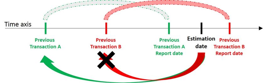
Report Days for the Real Estate Transaction
In Korea, a real estate transaction must be reported within 60 days from when the transaction
occurred, meaning that there may be transactions that occurred but have not been reported yet at
any date on which we want to estimate the price of an apartment (estimation date). In Figure 1,
there are two previous transaction A, B, but we can only identify the previous transaction A on a
specific estimation date because the previous transaction B has not been reported yet. To properly
incorporate this issue into the evaluation of the proposed and compared models, we excluded those
transactions that were reported after the estimation date from the test set in our consideration of
previous transactions (i.e., on our dataset, we did not use the previous transaction B in Figure 1 as an
instance of previous transaction so that the tested models could be directly applicable to the real world
usage settings in which those transactions that occurred but have not been reported yet at the time of
estimation would be not utilized as comparables).
Figure 1. A simplified example of possible previous transactions within the 60-day reporting period.
Report Days for Time-Variant Features
Aforementioned, we use two time-variant features—transaction volume and floating population.
Although the two datasets, transaction volume and floating population, are reported monthly, their
reporting dates are not equal. As a result of the differences in data gathering and preprocessing,
the data of transaction volume are generally published at the beginning of the month whereas the data
of floating population are typically published toward the end of the month. Therefore, we matched the
data of floating population in the previous month with that of transaction data.Sustainability 2020, 12, 5679 11 of 19
Date Difference between Transaction and Market Price
As mentioned before, the start date is treated as the transaction date. It means that the transaction
price has been recorded in every 1st, 11th, or 21st day of the month. As described earlier, the dataset
contains estimations of the apartment values made by real estate agents. These estimations are used to
assess the accuracy of the expert-based approach in our evaluation. However, the estimation dates in
this market price dataset do not necessarily match the sales transaction dates in the apartment sales
dataset. Therefore, each transaction in the sales dataset is mapped to the entry in the market price
dataset, which occurred earlier or on the same date. Table 9 shows the day differences between the
transaction date (in the sales dataset) and the market price estimation date (in the market price dataset)
in the two scenarios.
Table 9. The day differences between transaction date and market price estimation date.
Day Difference
Region Scenario
MAX MIN Median Mean STD †
1 4 0 3 2.14 1.37
Seoul
2 4 0 1 1.53 0.89
1 4 0 3 2.1 1.38
Geyonggi
2 4 0 1 1.6 1.12
STD † : Standard Deviation.
4.2. Methods
To implement the proposed approaches and assess the relative improvements made by the CSM
features, we used two gradient tree boosting methods, LightGBM [12] and CatBoost [13], each of
which was implemented in Python. Considering that it is difficult to trace how specific features affect
the estimation performance using a neural network modeling approach, we did not include a neural
network model in this experiment.
For comparison, we used two prices, “Common” and “MinMax” (average of the minimum and
the maximum estimates), derived from the market prices reported by the professional real estate
agents (two human-expert conditions). In addition, we included the baseline that uses only the
features covered in Section 4.1.3. This baseline (Basic condition) represents a regular machine learning
approach, exclusive of any CSM features. On top of the baseline, we test the additional effects of the
two types of CSM features (features from nearby apartment transactions and features from similar
price transactions), separately and jointly. Hence, we evaluate the performance improvement made
by each of the two types of CSM features and by the two types in combination, over and above the
baseline and the two human-expert estimation conditions (Common and MinMax).
4.3. Experiment Settings
For the two boosting methods, we use base parameter settings, except n_estimator. We set
n_estimator to 1000, objective to ‘Root Mean Square Error (RMSE)’ and subsample to 0.8 to avoid
overfitting. For CatBoost, we set bootstrap_type to ‘Bernoulli’. Then, we run the model 10 times for each
comparison case, and report the mean value of 10 trials and unpaired t-test statistic compared with the
Baseline (Basic (B)). Additionally, we empirically set the number of comparable sales features n to 5,
day interval m to 100, day offset α to 40, price offset β to 0.05.
4.4. Experiment Metrics
In our experiment, we used two evaluation criteria, Mean Absolute Percentage Error (MAPE)
and Root Mean Squared Percentage Error (RMSPE) because the average error value has different
magnitude by districts.Sustainability 2020, 12, 5679 12 of 19
• MAPE measures the average deviation of the predicted values out of the corresponding actual
values in percentage. More specifically, it is computed as,
N
1 yk − ŷk
MAPE = 100%
N ∑k yk
k (8)
k =1
where N is the number of apartment transactions, ŷk is the predicted kth value and yk is the
corresponding actual value.
• RMSPE measures the standard deviation of the predicted values out of the corresponding actual
values in percentage. Compared to MAPE, this measure more heavily penalizes outliers. It is
computed as, v
u 1 N y − ŷk
u
RMSPE = 100%t ∑ ( k )2 (9)
N k =1 yk
where N is the number of apartment transactions, ŷk is the predicted kth value and yk is the
corresponding actual value.
Additionally, for practical reasons, we also present cumulative percentage of 10% errors as the
practitioners in this field commonly use this criterion.
4.5. Performance Results
The experimental results consistently show that the machine learning models are superior to the
human expert estimations. In terms of MAPE (Table 10), RMSPE (Table 11), and cumulative percentage
of 10% (Table 12), the machine learning models we developed produce more accurate predictions of
apartment transaction prices than the prices estimated by the real estate professionals (i.e., Market
Price in Tables 10–12). The professionals are those who work in a real estate office located closely to
the apartment complex, serving as mediaries for the sales and purchase transactions of the apartments
in the complex. The largest bank in Korea, KB Kookmin Bank, relies on a massive number of these real
estate agents to produce and update its assessment of those real estate properties every week, sharing
that information with other major banks across the country, which is then used for determining the
maximum amount of mortgage loan associated with the real estate property. Our automated approach
is a much more efficient yet less biased solution as evidenced through MAPE, RMSPE, and cumulative
percentage of 10%.
For Seoul and Gyeonggi, adding the full set of CSM-derived price features showed the highest
improvement over the baseline in comparison to the conditions where only the nearby apartment
transaction or similar price transaction features were added, confirming that the additional features
based on CSM have positive effects on improving the prediction accuracy of apartment prices, over and
above the regular machine learning approach, and the nearby apartment transaction features and the
similar price transaction features have independent effects, lending themselves to greater effects when
combined together. In terms of MAPE, we confirmed that there were significant improvements in
all of the comparison cases based on the t-test results. Hence, in RMSPE and cumulative percentage,
almost all of the comparison cases showed significant improvements according to the t-test results,
and some slight improvements were still observable even when not significant. In addition, the baseline
condition mostly shows worse estimation than the market price estimation by human experts in terms
of RMSPE. It also shows that the baseline approach generates higher variance estimation than the
market price estimation. In contrast, the addition of the CSM features in combination (baseline plus
nearby features plus similar price features) shows positive effects on decreasing variance regardless of
scenarios or districts, relative to the estimations made by human experts and to the baseline models,
without exception.Sustainability 2020, 12, 5679 13 of 19
Table 10. The Mean Absolute Percentage Error (MAPE) results of Seoul and Gyeonggi in Scenarios 1 and 2.
MAPE Market Price Baseline Ours
Boosting
District Scenarios Common MinMax Basic (B) B + Nearby (N) B + Similar (S) B+N+S
LightGBM 6.42 6.19 *** 5.84 *** 5.68 ***
Scenario 1 6.28 6.35
CatBoost 6.03 5.99 *** 5.49 *** 5.41 ***
Seoul
LightGBM 8.89 8.57 *** 7.97 *** 7.75 ***
Scenario 2 7.99 8.07
CatBoost 8.34 8.15 *** 7.2 *** 7.14 ***
LightGBM 4.86 4.83 *** 4.82 *** 4.79 ***
Scenario 1 5.44 5.47
CatBoost 4.96 4.93 *** 4.98 *** 4.94 ***
Gyoenggi
LightGBM 5.37 5.32 ** 5.28 *** 5.22 ***
Scenario 2 5.78 5.83
CatBoost 5.41 5.37 *** 5.38 *** 5.33 ***
** p < 0.01, *** p < 0.001: Significance of the difference test made in relation to the basic (B) baseline condition.
Table 11. The Root Mean Squared Percentage Error (RMSPE) results of Seoul and Gyeonggi in Scenarios 1 and 2.
RMSPE Market Price Baseline Ours
Boosting
District Scenarios Common MinMax Basic (B) B + Nearby (N) B + Similar (S) B+N+S
LightGBM 8.39 8.13 *** 7.71 *** 7.54 ***
Scenario 1 7.89 7.95
CatBoost 8.13 8.07 *** 7.53 *** 7.42 ***
Seoul
LightGBM 11.1 10.78 *** 10.04 *** 9.82 ***
Scenario 2 10.3 10.36
CatBoost 10.69 10.49 *** 9.38 *** 9.31 ***
LightGBM 6.9 6.87 *** 6.84 *** 6.8 ***
Scenario 1 7.81 7.84
CatBoost 7.15 7.1 *** 7.14 7.08 ***
Gyoenggi
LightGBM 11.31 11.3 11.26 11.23 ***
Scenario 2 11.4 11.29
CatBoost 11.44 11.4 *** 11.42 * 11.37 ***
* p < 0.05, *** p < 0.001: Significance of the difference test made in relation to the basic (B) baseline condition.Sustainability 2020, 12, 5679 14 of 19
Table 12. The cumulative percentage of 10% errors results of Seoul and Gyoenggi in Scenarios 1 and 2.
Cumulative Percentage Market Price Baseline Ours
Boosting
District Scenarios Common MinMax Basic (B) B + Nearby (N) B + Similar (S) B+N+S
LightGBM 79.18 80.73 *** 82.76 *** 83.78 ***
Scenario 1 81.45 81.21
CatBoost 81.46 81.72 *** 84.83 *** 85.54 ***
Seoul
LightGBM 62.94 65.05 *** 68.44 *** 69.91 ***
Scenario 2 69.31 68.93
CatBoost 67.14 67.69 * 73.49 *** 73.95 ***
LightGBM 89.0 89.21 *** 89.24 *** 89.41 ***
Scenario 1 86.58 86.52
CatBoost 88.31 88.47 *** 88.09 *** 88.35
Gyoenggi
LightGBM 86.27 86.55 ** 86.74 *** 87.05 ***
Scenario 2 84.5 84.35
CatBoost 85.98 86.16 ** 86.18 *** 86.44 ***
* p < 0.05, ** p < 0.01, *** p < 0.001: Significance of the difference test made in relation to the basic (B) baseline condition.Sustainability 2020, 12, 5679 15 of 19
CSM-derived price features show different impacts on the estimation of housing prices.
Specifically, CSM-derived price features based on the similar price transaction assumption reveal
more positive predictive efficacy than those features based on the nearby transaction assumption,
probably due to the fact that similarly priced apartments appeal to similar groups of people and that
they share some common features that contribute to the formation of their comparable prices. Further,
between the two boosting techniques of LightGBM and CatBoost, the results show that LightGBM is a
better performer for Gyoenggi and CatBoost is a better performer for Seoul, consistently for all of the
performance metrics used in this study.
5. Discussion
For future smart cities, computational approaches to the estimation of real estate properties on a
large scale are likely to be essential for intelligent planning and policy making [4,5]. In this study, we
explored the possibility of applying comparable sales method (CSM) to the automated price estimation
of real estate properties. To the best of our knowledge, no attempt has been made to apply CSM to
the automated estimation of house prices. The study results consistently show that the computational
approaches developed in this research are superior to human-based approaches in the low and high
fluctuation periods of time. Furthermore, among the computational approaches, this study shows
that the CSM-based approaches, particularly involving both the nearby-located comparables and
similarly-priced comparables, are superior to the traditional machine learning approaches.
The objective of this study was to develop a computational method that can implement the idea
of CSM currently used by real estate experts. In doing so, we have articulated two approaches that can
help us locate effective comparables in the market. One approach is to consider proximity information
on nearby apartment transactions. To accurately identify those nearby comparables, we utilized not
only distance information, but also intrinsic and transaction characteristics. This approach more closely
resembles the current practices involving human assessors. Unlike the previous approach, the other
approach is to consider past price information and use it to identify comparable properties that can
serve as the references against the price fluctuations over time.
The proposed method of CSM may be implemented as an extension of the Ordinary Least Squares
(OLS) methodology. Then, CSM can provide additional perspectives on expanding the variable set and
explicating the model’s estimation results. However, because the model assumes that the variables are
linearly related, the performance is likely to suffer. In general, boosting-based methodologies show
significantly higher predictive performance than other conventional methodologies [42–44].
In conclusion, in this paper we propose a novel approach inspired by CSM to infer the prices of
similar properties and use them as predictors of apartment transaction prices. In order to measure
the predictive power of the newly proposed features, we collected the apartment sales dataset for
the capital city and the largest province in Korea, and constructed machine learning models with
alternative combinations of features. The experiment results show that the proposed CSM-based
approaches are superior when compared with the traditional methods involving human experts or
to the regular machine learning approach that uses both internal and external factors excluding the
CSM-derived features. Based on the significant results found by this research, the proposed method
that incorporates the two types of CSM features in combination is currently under development by KB
Kookmin Bank for its public service. In our future work, we plan to expand the prediction model by
incorporating other types of information such as news articles and policy changes and by applying
deep learning approaches to the modelling of comparable sales features.
Author Contributions: Conceptualization, Y.K. and M.Y.Y.; methodology, Y.K.; software, Y.K. and S.C.; validation,
Y.K., S.C. and M.Y.Y.; formal analysis, Y.K.; data curation, S.C.; writing—original draft preparation, S.C.;
writing—review and editing, M.Y.Y.; supervision, M.Y.Y.; project administration, M.Y.Y.; funding acquisition,
M.Y.Y. All authors have read and agreed to the published version of the manuscript.Sustainability 2020, 12, 5679 16 of 19 Funding: The work reported in this paper is an extension of the outcome of a research project funded by KB Kookmin Bank. Conflicts of Interest: The authors declare no conflict of interest. Abbreviations The following abbreviations are used in this manuscript: CSM Comparable Sales Method SVM Support Vector Machines LSTM Long Short-Term Memory ZHVI Zillow Home Value Index MOLIT The Ministry of Land, Infrastructure, and Transport KAB Korea Appraisal Board KOSIS Korean Statistical Information Service MAPE Mean Absolute Percentage Error RMSPE Root Mean Squared Percentage Error RMSE Root Mean Square Error Appendix A. Algorithms Algorithm A1 Extracting neighboring buildings Input: Set of apartment buildings A, buildings coordinate pairs C, number of neighbors to find n Output: Apartment buildings and n neighbors mapping A0 1: function F IND N EIGHBORS (A, n) 2: for i = 0 to length( A) do 3: building ← Ai 4: distances ← [] 5: for j = 0 to length( A) do 6: distance ← EuclideanDistance(Ci ,Cj ) 7: distances ← append distance 8: neighbors ← GetTopN_ClosestBuildings(A, distances, n) 9: A0 ← append (building, neighbors) 10: return A0 Algorithm A2 Extracting nearby apartment prices 1: function G ET P RICE(neighbors j , T, curr apartment ) 2: apartments_ f ← GetNeighborApartment’s_features(neighbors j , T) 3: max_similarity ← 0 4: price ← 0 5: for i = 0 to length( apartments_ f ) do 6: similarity ← CosineSimilarity(curr apartment , apartments_ f i ) 7: if similarity > max_similarity then 8: max_similarity ← similarity 9: price ← apartments_ f i [ price] 10: return price
Sustainability 2020, 12, 5679                                                                     17 of 19

Algorithm A3 Adding prices of nearby apartments
Input: Buildings and neighbors mapping A0 , set of apartments T
Output: Set of apartments with comparable sales features T 0
 1: function A DD A PARTMENTS P RICE F EATURES (A0 , T)
 2:    for i = 0 to length( T ) do
 3:        neighbors ← ExtractNeighbors(A0 , Ti )
 4:        price_ f eatures ← []
 5:        for j = 0 to length(neighbors) do
 6:            price ← GetPrice(neighbors j , T, Ti )
 7:            price_ f eatures ← append price
 8:        T 0 ← append ( Ti , price_ f eatures)
 9:    return T 0

Algorithm A4 Adding similar price features
Input: Transaction A, list of transactions B in the apartments different from A0 s apartment, number of
     price features n to be added, m day interval, day offset α to define valid time period for searching
     similar prices, price offset P to define price boundaries within which price is considered similar,
    a set of KB Index
Output: list of similar price features F for transaction A
 1: function A DD S IMILAR P RICE F EATURES (A, B, n, m, α, β, KB Index)
 2:     F ← []
 3:     candidates ← []
 4:     A prev ← GetPreviousTransaction(A)
 5:     prev_price ← A prev [ price]
 6:     prev_date ← A prev [date]
 7:     if prev_date_interval > m then
 8:          search_start ← prev_date − α
 9:          search_end ← prev_date + α
10:          lower ← prev_price × (1 − β)
11:          upper ← prev_price × (1 + β)
12:          for i = 0 to length( B) do
13:              transaction ← Bi
14:              price ← transaction[ price]
15:              date ← transaction[date]
16:              is_valid_date ← False
17:              is_valid_price ← False
18:              if date > search_start & date < search_end then
19:                   is_valid_date ← True
20:              if price > lower & price < upper then
21:                   is_valid_price ← True
22:              if is_valid_date & is_valid_price then
23:                   candidates ← append price
24:     if isEmpty(candidates) then
25:          for i = 0 to length(n) do
26:              F ← append previous_price
27:     else
28:          candidates ← GetTopNtransacions(candidates,prev_price,n)
29:          for i = 0 to length(n) do
30:              F ← append candidatesi ∗ KBKB   Indexneardate
                                               Indexnearprev_date
31:          return F
Sustainability 2020, 12, 5679 18 of 19
References
1. Demyanyk, Y.; Van Hemert, O. Understanding the subprime mortgage crisis. Rev. Financ. Stud. 2009,
24, 1848–1880. [CrossRef]
2. Cerutti, E.; Dagher, J.; Dell’Ariccia, G. Housing finance and real-estate booms: A cross-country perspective.
J. Hous. Econ. 2017, 38, 1–13. [CrossRef]
3. Northcraft, G.B.; Neale, M.A. Experts, amateurs, and real estate: An anchoring-and-adjustment perspective
on property pricing decisions. Organ. Behav. Hum. Decis. Process. 1987, 39, 84–97. [CrossRef]
4. Pettit, C.; Bakelmun, A.; Lieske, S.N.; Glackin, S.; Thomson, G.; Shearer, H.; Dia, H.; Newman, P. Planning
support systems for smart cities. City Cult. Soc. 2018, 12, 13–24. [CrossRef]
5. Soomro, K.; Bhutta, M.N.M.; Khan, Z.; Tahir, M.A. Smart city big data analytics: An advanced review.
Wiley Interdiscip. Rev. Data Min. Knowl. Discov. 2019, 9, e1319. [CrossRef]
6. Borst, R.; McCluskey, W. Comparative evaluation of the comparable sales method with geostatistical
valuation models. Pac. Rim Prop. Res. J. 2007, 13, 106–129. [CrossRef]
7. Cupal, M. The Comparative Approach theory for real estate valuation. Procedia-Soc. Behav. Sci. 2014,
109, 19–23. [CrossRef]
8. Park, B.; Bae, J.K. Using machine learning algorithms for housing price prediction: The case of Fairfax
County, Virginia housing data. Expert Syst. Appl. 2015, 42, 2928–2934. [CrossRef]
9. Ren, Y.; Fox, E.B.; Bruce, A. Clustering correlated, sparse data streams to estimate a localized housing price
index. Ann. Appl. Stat. 2017, 11, 808–839. [CrossRef]
10. Korea Appraisal Board. Korea Real Estate Market Report Vol.9. 2019. Available online: http://www.kab.co.
kr/kab/home/eng/trend/trend02.jsp (accessed on 21 June 2020).
11. Ministry of Land, Infrastructure and Transport (MOLIT). Transaction Price Open System. 2019. Available
online: http://rt.molit.go.kr/ (accessed on 21 June 2020).
12. Ke, G.; Meng, Q.; Finley, T.; Wang, T.; Chen, W.; Ma, W.; Ye, Q.; Liu, T.Y. LightGBM: A highly efficient gradient
boosting decision tree. In Proceedings of the Neural Information Processing Systems 2017, Long Beach, CA,
USA, 4–9 December 2017; pp. 3146–3154.
13. Prokhorenkova, L.; Gusev, G.; Vorobev, A.; Dorogush, A.V.; Gulin, A. CatBoost: Unbiased boosting with
categorical features. In Proceedings of the Neural Information Processing Systems 2018, Montreal, QC,
Canada, 3–8 December 2018; pp. 6638–6648.
14. Xiao, Y. Hedonic housing price theory review. In Urban Morphology And Housing Market; Springer: Singapore,
2017; pp. 11–40.
15. Mirkatouli, J.; Samadi, R.; Hosseini, A. Evaluating and analysis of socio-economic variables on land and
housing prices in Mashhad, Iran. Sustain. Cities Soc. 2018, 41, 695–705. [CrossRef]
16. Hussain, T.; Abbas, J.; Wei, Z.; Nurunnabi, M. The Effect of Sustainable Urban Planning and Slum Disamenity
on The Value of Neighboring Residential Property: Application of The Hedonic Pricing Model in Rent Price
Appraisal. Sustainability 2019, 11, 1144. [CrossRef]
17. Čeh, M.; Kilibarda, M.; Lisec, A.; Bajat, B. Estimating the performance of random forest versus multiple
regression for predicting prices of the apartments. ISPRS Int. J. Geo-Inf. 2018, 7, 168. [CrossRef]
18. Gu, J.; Zhu, M.; Jiang, L. Housing price forecasting based on genetic algorithm and support vector machine.
Expert Syst. Appl. 2011, 38, 3383–3386. [CrossRef]
19. Bin, J.; Tang, S.; Liu, Y.; Wang, G.; Gardiner, B.; Liu, Z.; Li, E. Regression model for appraisal of real estate
using recurrent neural network and boosting tree. In Proceedings of the 2017 2nd IEEE International
Conference on Computational Intelligence and Applications (ICCIA), Beijing, China, 8–11 September 2017;
pp. 209–213.
20. Poursaeed, O.; Matera, T.; Belongie, S. Vision-based real estate price estimation. Mach. Vis. Appl. 2018,
29, 667–676. [CrossRef]
21. Bency, A.J.; Rallapalli, S.; Ganti, R.K.; Srivatsa, M.; Manjunath, B. Beyond Spatial Auto-Regressive Models:
Predicting Housing Prices with Satellite Imagery. In Proceedings of the 2017 IEEE Winter Conference on
Applications of Computer Vision (WACV), Santa Rosa, CA, USA, 24–31 March 2017; pp. 320–329.
22. Law, S.; Paige, B.; Russell, C. Take a look around: Using street view and satellite images to estimate house
prices. ACM Trans. Intell. Syst. Technol. 2019, 10, 1–19. [CrossRef]Sustainability 2020, 12, 5679 19 of 19
23. Bradley, J.; Amde, M. Random Forests and Boosting in MLlib. 2015. Available online: https://databricks.
com/blog/2015/01/21/random-forests-and-boosting-in-mllib.html (accessed on 21 June 2020).
24. Ogutu, J.O.; Piepho, H.P.; Schulz-Streeck, T. A comparison of random forests, boosting and support vector
machines for genomic selection. BMC Proc. 2011, 5, 11. [CrossRef]
25. Chen, T.; Guestrin, C. XGBoost: A Scalable Tree Boosting System. In Proceedings of the KDD ’16,
San Francisco, CA, USA, 13–17 August 2016; pp. 785–794.
26. Barone, A. Comparative Market Analysis. 2019. Available online: https://www.investopedia.com/terms/
c/comparative-market-analysis.asp (accessed on 21 June 2020).
27. Borst, R.A.; McCluskey, W. The modified comparable sales method as the basis for a property tax valuations
system and its relationship and comparison to spatially autoregressive valuation models. In Mass Appraisal
Methods: An International Perspective for Property Valuers; Wiley: Hoboken, NJ, USA, 2008; pp. 49–69.
28. Collins, G. Groundwater Valuation in Texas: The Comparable Transactions Method. In Rice University’s
Baker Institute FOR Public Policy Report; James, A., Ed.; Baker III Institute for Public Policy of Rice University:
Houston, TX, USA, 2018.
29. Healy, M.; Bergquist, K. The sales comparison approach and timberland valuation. Apprais. J. 1994, 62, 587.
30. KB Kookmin Bank. Market Price Open System. 2019. Available online: https://onland.kbstar.com/
(accessed on 21 June 2020).
31. Hochreiter, S.; Schmidhuber, J. Long short-term memory. Neural Comput. 1997, 9, 1735–1780. [CrossRef]
32. Chollet, F. Keras. 2015. Available online: https://keras.io (accessed on 21 June 2020).
33. Davis, M.A.; Palumbo, M.G. The Price of Residential Land in Large US Cities. J. Urban Econ. 2008, 63, 352–384.
[CrossRef]
34. Young Yoon, J. Gov’t Renews War on Real Estate Speculation. 2018. Available online: https://www.
koreatimes.co.kr/www/biz/2018/12/367_254423.html (accessed on 21 June 2020).
35. Charles, L.; Garion, L.; Youngman, L. Testing alternative theories of the property price-trading volume
correlation. J. Real Estate Res. 2002, 23, 253–264.
36. De Wit, E.R.; Englund, P.; Francke, M.K. Price and transaction volume in the Dutch housing market. Reg. Sci.
Urban Econ. 2013, 43, 220–241. [CrossRef]
37. Wang, X.R.; Hui, E.C.M.; Sun, J.X. Population migration, urbanization and housing prices: Evidence from
the cities in China. Habitat Int. 2017, 66, 49–56. [CrossRef]
38. Xue, C.; Ju, Y.; Li, S.; Zhou, Q. Research on the Sustainable Development of Urban Housing Price Based on
Transport Accessibility: A Case Study of Xi’an, China. Sustainability 2020, 12, 1497. [CrossRef]
39. Machin, S. Houses and schools: Valuation of school quality through the housing market. Labour Econ. 2011,
18, 723–729. [CrossRef]
40. Lan, F.; Wu, Q.; Zhou, T.; Da, H. Spatial Effects of Public Service Facilities Accessibility on Housing Prices:
A Case Study of Xi’an, China. Sustainability 2018, 10, 4503. [CrossRef]
41. Park, J.H.; Lee, D.K.; Park, C.; Kim, H.G.; Jung, T.Y.; Kim, S. Park accessibility impacts housing prices in
Seoul. Sustainability 2017, 9, 185. [CrossRef]
42. Cinar, U.K. Combining Domain Knowledge & Machine Learning: Making Predictions using Boosting
Techniques. In Proceedings of the 2019 3rd International Conference on Advances in Artificial Intelligence,
Istanbul, Turkey, 22–24 October 2019; pp. 9–13.
43. Chen, L.; Yao, X.; Liu, Y.; Zhu, Y.; Chen, W.; Zhao, X.; Chi, T. Measuring Impacts of Urban Environmental
Elements on Housing Prices Based on Multisource Data—A Case Study of Shanghai, China. ISPRS Int. J.
Geo-Inf. 2020, 9, 106. [CrossRef]
44. Sangani, D.; Erickson, K.; Al Hasan, M. Predicting zillow estimation error using linear regression and
gradient boosting. In Proceedings of the 2017 IEEE 14th International Conference on Mobile Ad Hoc and
Sensor Systems (MASS), Orlando, FL, USA, 22–25 October 2017; pp. 530–534.
c 2020 by the authors. Licensee MDPI, Basel, Switzerland. This article is an open access
article distributed under the terms and conditions of the Creative Commons Attribution
(CC BY) license (http://creativecommons.org/licenses/by/4.0/).You can also read